X-ray energies of circular transitions and electrons screening in kaonic atoms

Abstract

The QED contribution to the energies of the circular $(n,\ell=n-1)$, $2\leq n\leq 19$ transitions have been calculated for several kaonic atoms throughout the periodic table, using the current world average kaon mass. Calculations were done in the framework of the Klein-Gordon equation, with finite nuclear size, finite particle size, and all-order Uelhing vacuum polarization corrections, as well as Källén and Sabry and Wichmann and Kroll corrections. These energy level values are compared with other computed values. The circular transition energies are compared with available measured and theoretical transition energy. Electron screening is evaluated using a Dirac-Fock model for the electronic part of the wave function. The effect of electronic wavefunction correlation is evaluated for the first time.

I Introduction

An exotic atom is formed when a particle, with a negative charge and long-enough lifetime, slows down and stops in matter. It can then displace an atomic electron, and become bound in a high principal quantum number atomic orbital around the nucleus. The principal quantum number of this highly excited state is of the order of $n=\sqrt{m/m_{e}}$, where $m$ and $m_{e}$ are the masses of the particle and of the electron, respectively Horvath (1994). The higher the overlap between the wave functions of the electron and the particle, the more probable is the formation of an exotic atom Horvath (1994).

The exotic atoms formed in this way are named after the particle forming them. It the particle is a the negative kaon $K^{-}$, a meson with a spin-0 and a lifetime of 1.237$\times 10^{-8}$ s, a kaonic atom is thus created.

Because the particle mass, and thus transition energies are so much higher that the electron’s (a kaon is $\approx$964 times heavier than an electron), the de-excitation of the exotic atom will start via Auger processes, in a process equivalent to internal conversion for $\gamma$-rays, while the level spacing is small and there are electrons to be ejected, and then via radiative ($E1$) transitions, producing characteristic X-rays while cascading down its own sequence of atomic levels until some state of low principal quantum number. One thus can end with a completely striped atom, provided the mass of the exotic particle is large and the atomic number of the atom not too high.

The initial population of the atomic states is related to the available density of states, so for any given principal quantum number $n$ the higher orbital momenta are favored to some extent because of their larger multiplicity. As the Auger transitions do not change the shape of the angular momentum distribution, the particle quickly reaches the ($\ell=n-1$) orbits Horvath (1994). Once the radiative ($E1$) transitions begin to dominate, we have the selection rule $\Delta\ell=\pm 1$, often with many possible values of $\Delta n$ being important. Under such a scheme, the kaons in low angular momentum orbits will rapidly reach orbitals with a sizable overlap with the nucleus and be captured. Soon mostly the circular orbitals $(n,\ell=n-1)$ from which only transitions to other circular orbits can occur, ($n$, $\ell=n-1$) $\rightarrow$($n-1$, $\ell=n-2$), will be populated. The so-called parallel transition ($n$, $\ell=n-2$) $\rightarrow$($n-1$, $\ell=n-3$) is much weaker.

Finally the particle in a state of low angular momentum will be absorbed by the nucleus through the kaon-nucleus strong interaction. This strong interaction causes a shifting of the energy of the lowest atomic level from its purely electro-magnetic value while the absorption reduces the lifetime of the state and so X-ray transitions to this final atomic level are broadened.

Therefore, following the stopping of the kaon in matter, well-defined states of a kaonic atom are established and the effects of the kaon-nucleus strong interaction can be studied. The overlap of the atomic orbitals with the nucleus covers a wide range of nuclear densities thus creating a unique source of information on the density dependence of the hadronic interaction.

Here we are concerned with levels in which the effect of the strong interaction is negligible, to study the atomic structure. Our objective is to provide highly accurate values of high-angular momentum circular transition, which can be useful for experiment in which internal calibration lines, free from strong interaction shifts and broadening are needed, as has been done in the case of pionic and antiprotonic atoms Lenz et al. (1998); Hauser et al. (1998); Gotta et al. (1999); Siems et al. (2000). Our second objective is to study the electron screening, i.e., the change in the energy of the kaon due to the presence of a few remaining electrons, in a relativistic framework.

In general, although the kaonic atom energy is dominated by the Coulomb interaction between the hadron and the nucleus, one must take into account the strong-interaction between the kaon and the nucleus when the kaon and nuclear wave function overlap. As our aim is to provide highly accurate QED-only values, that can be used to extract experimental strong-interaction shifts from energy measurements. We refer the interested reders to the literature, e.g., Refs. Friedman and Gal (1999); Friedman et al. (1994); Batty (1981).

Exotic X-ray transitions have been intensively studied for decades as they can provide the most precise and relevant physical information for various fields of interest. This study is pursued at all major, intermediate energy accelerators where mesons are produced: at the AGS of Brookhaven National Laboratory (USA), at JINR (Dubna, Russia), at LAMPF, the Los Alamos Meson Physics Facility (Los Alamos, USA), at LEAR, the Low Energy Antiproton Ring of CERN (Geneva, Switzerland), at the Meson Science Laboratory of the University of Tokyo (at KEK, Tsukuba, Japan), at the Paul Scherrer Institute (Villigen, Switzerland), at the Rutherford Appleton Laboratory (Chilton, England), at the Saint-Petersburg Nuclear Physics Institute (Gatchina, Russia), and at TRIUMF (Vancouver, Canada) Horvath (1994).

It is now planed, in the context of the DEAR experiment (strong interaction shift and width in kaonic hydrogen) on DA$\Phi$NE in Frascati Maiani (1997); Guaraldo et al. (1999) to measure some other transitions of kaonic atoms, such as the kaonic nitrogen, aluminum, titanium, neon, and silver. Similar work is under way at KEK.

The measurements concerning the exotic atoms permit the extraction of precise information about the orbiting particle Batty et al. (1989a), such as charge/mass ratio, and magnetic moment, and the interaction of such particles with nuclei. In addition, properties of nuclei Batty et al. (1989b), such as nuclear size, nuclear polarization, and neutron halo effects in heavy nuclei Lubinski et al. (1994), have been studied. Furthermore, the mechanism of atomic capture of such heavy charged particles and atomic effects such as Stark mixing Batty (1989) and trapping Morita et al. (1994) have been studied extensively.

Furthermore, as the X-ray transition energies are proportional to the reduced mass of the system, studies in the intermediate region of the atomic cascade were used to measure the masses of certain negative particles. In order to minimize the strong interactions for the mass determination it is considered only transitions between circular orbits ($n,n-1$)$\rightarrow$($n-1,n-2$) far from the nucleus Kunselman (1971).

In this paper, we calculate the orbital binding energies of the kaonic atoms for $1\leq Z\leq 92$ and $0\leq\ell\leq 12$ for circular states and $1\leq\ell\leq 11$ for parallel near circular states by the resolution of the Klein-Gordon equation (KGE) including QED corrections.

The paper is organized as follows. The principle of the calculation is outlined in Sec. II. The results obtained in this work are given in Sec. III. Finally we give our conclusions in Sec. IV.

II Calculation of the energy levels

II.1 Principle of the calculation

Because of the much larger mass of the particle, its orbits are much closer to the central nucleus than those of the electrons. In addition, since there is only one heavy particle, the Pauli principle does not play a role and the whole range of classical atomic orbits are available. As a result, to first order, the outer electrons can be ignored and the exotic atom has many properties similar to those of the simple, one-electron hydrogen atom Batty (1995). Yet there are cases where the interaction between the electron shell and the exotic particle must be considered. Over the year the MCDF code of Desclaux and Indelicato Desclaux (1975, 1993) was modified so that it could accommodate a wavefunction that is the product of a Slater determinant for the electron, by the wavefunction of an exotic particle. In the case of spin 1/2 fermions, this can be done with the full Breit interaction. In the case of spin 0 bosons, this is restricted to the Coulomb interaction only. With that code it is then possible to investigates the effects of changes in the electronic wavefunction, e.g., due to correlation on the kaonic transitions. It is also possible to take into account specific properties of the exotic particle like its charge distribution radius. The different contributions to the final energy are described in more details in this section.

II.2 Numerical solution of the Klein-Gordon equation

Since kaons are spin-0 bosons, they obey the Klein Gordon equation, which in the absence of strong interaction may be written, in atomic units, as

$$\left[\alpha^{2}\left(E-V_{c}(r)\right)^{2}+{\vec{\nabla}}^{2}-\mu^{2}c^{2}\right]\psi\left(\mathbf{r}\right)=0,$$ (1)

where $\mu$ is the kaon reduced mass, $E$ is the Kaon total energy, $V_{c}$ is the sum of the Coulomb potential, describing the interaction between the kaon and the finite charge distribution of the nucleus, of the Uehling vacuum-polarization potential (of order $\alpha\left(\alpha Z\right)$) Uehling (1935) and of the potential due to the electrons. Units of $\hbar=c=1$ are used. For a spherically symmetric potential $V_{c}$, the bound state solutions of the KG equation (1) are of the usual form $\psi_{n\ell m}\left(\mathbf{r}\right)=Y_{\ell m}\left(\theta,\phi\right)\left(p_{n\ell}\left(r\right)/r\right)$. Compared to the numerical solution of the Dirac-Fock equation Desclaux (1993), here we must take care of the fact that the equation is quadratic in energy. The radial differential equation deduced from (1) is rewritten as a set of two first-order equations

$$\frac{d}{dr}p = q$$

$$\frac{d}{dr}q = \left[\mu c^{2}+\frac{\ell(\ell+1)}{r^{2}}-\alpha^{2}\left(V_{c}-E\right)^{2}\right]p,$$ (2)

where $p=p(r)$ is the radial KG wave function. Following Ref. Desclaux (1993) the equation is solved by a shooting method, using a predictor-corrector method for the outward integration up to a point $r_{m}$ which represents the classical turning point in the potential $V_{c}$. The inward integration uses finite differences and the tail correction and provide a continuous $p$ as well as a practical way to fix how far out one must start the integration to solve Eq.  (II.2) within a given accuracy. The eigenvalue $E$ is found by requesting that $q$ is continuous at $r_{m}$. If we suppose that $q$ is not continuous, then an improved energy $E$ is obtained by a variation of $p$ and $q$, such that

$$(q+\delta q)_{r_{m}^{+}}=(q+\delta q)_{r_{m}^{-}}.$$ (3)

To find the corresponding $\delta E$ we replace $p$, $q$ and $E$ by $p+\delta p$, $q+\delta q$ and $E+\delta E$ in Eq. (II.2). Keeping only first order terms we get

$$\frac{d}{dr}p+\frac{d}{dr}\delta p = q+\delta q$$ (4)

$$\frac{d}{dr}\delta q = \left[\mu c^{2}+\frac{\ell(\ell+1)}{r^{2}}-\alpha^{2}\left(V_{c}-E\right)^{2}\right]\delta p$$ (5)

$$+2\alpha^{2}(V-E)\delta Ep.$$

Multiplying Eq. (4) by $q$ and Eq. (5) by $p$, subtracting the two equations, and using the original differential equation (II.2) whenever possible we finally get

$$\frac{d}{dr}(p\delta q-q\delta p)=2\alpha^{2}\left(V_{c}-E\right)p^{2}\delta E.$$ (6)

Combining Eqs. (3), (6), integrating, using the fact that $p$ is continuous everywhere, and neglecting higher-order corrections, we finally get

$$\delta E=\frac{p(r_{m})\left[q(r_{m}^{+})-q(r_{m}^{-})\right]}{2\alpha^{2}\int_{0}^{\infty}\left(V_{c}-E\right)p^{2}dr}.$$ (7)

In the case of the Dirac equation one would get

$$\delta E=\frac{p(r_{m})\left[q(r_{m}^{+})-q(r_{m}^{-})\right]}{\alpha\left[\int_{0}^{r_{m}^{-}}(p^{2}+q^{2})dr+\int_{r_{m}^{+}}^{\infty}(p^{2}+q^{2})dr\right]},$$ (8)

where $p$ and $q$ are the large and small components, and the integral in the denominator remain split because $q$ is not continuous, but is converging toward 1, as it is the norm of the wave function. In both cases one can use Eq. (7) or (8) to obtain high-accuracy energy and wave function by an iterative procedure, checking the number of node to insure convergence toward the right eigenvalue.

II.3 Nuclear structure

For heavy elements, a change between a point-like and an extended nuclear charge distribution strongly modifies the wave function near the origin. One nuclear contribution is easily calculated by using a finite charge distribution in the differential equations from which the wave function are deduced. For atomic number larger than 45 we use a Fermi distribution with a thickness parameter $t=2.3$ fm and a uniform spherical distribution otherwise. The most abundant naturally-occurring isotope was used.

In Table 1 we list the nuclear parameters used in the presented calculations in atomic units.

Table 1: Nuclear parameters used in this work in atomic units

Z	Nuclear Radius	Mean Square Radius	Reduced Mass
1	$2.102958\times 10^{-5}$	$1.628944\times 10^{-5}$	$633.030$
2	$4.081494\times 10^{-5}$	$3.161512\times 10^{-5}$	$853.110$
3	$5.838025\times 10^{-5}$	$4.522115\times 10^{-5}$	$898.234$
4	$6.145418\times 10^{-5}$	$4.760220\times 10^{-5}$	$912.431$
6	$5.989282\times 10^{-5}$	$4.639278\times 10^{-5}$	$925.227$
13	$7.418903\times 10^{-5}$	$5.746657\times 10^{-5}$	$947.486$
14	$7.579918\times 10^{-5}$	$5.871379\times 10^{-5}$	$948.135$
17	$8.136153\times 10^{-5}$	$6.302237\times 10^{-5}$	$951.674$
19	$8.384263\times 10^{-5}$	$6.494422\times 10^{-5}$	$953.134$
20	$8.496485\times 10^{-5}$	$6.581349\times 10^{-5}$	$953.453$
22	$8.780214\times 10^{-5}$	$6.801124\times 10^{-5}$	$955.537$
28	$9.241059\times 10^{-5}$	$7.158094\times 10^{-5}$	$957.342$
29	$9.509662\times 10^{-5}$	$7.366153\times 10^{-5}$	$958.031$
42	$1.073460\times 10^{-4}$	$8.314984\times 10^{-5}$	$960.899$
45	$1.098320\times 10^{-4}$	$8.507547\times 10^{-5}$	$961.150$
60	$1.101005\times 10^{-4}$	$9.287059\times 10^{-5}$	$962.506$
74	$1.221443\times 10^{-4}$	$1.015048\times 10^{-4}$	$963.325$
82	$1.256895\times 10^{-4}$	$1.040691\times 10^{-4}$	$963.645$
92	$1.348635\times 10^{-4}$	$1.107455\times 10^{-4}$	$963.955$

II.4 QED effects

II.4.1 Self-consistent Vacuum Polarization

A complete evaluation of radiative corrections in kaonic atoms is beyond the scope of the present work. However the effects of the vacuum polarization in the Uehling approximation, which comes from changes in the bound-kaon wave function, can be relatively easily implemented in the framework of the resolution of the KGE using a self-consistent method.

In practice one only need to add the Uehling potential to the nuclear Coulomb potential, to get the contribution of the vacuum polarization to the wave function to all orders, which is equivalent to evaluate the contribution of all diagrams with one or several vacuum polarization loop of the kind displayed on Fig. 1. For the exact signification of these diagrams see, e.g., Schneider et al. (1994); Blundell et al. (1997); Mohr et al. (1998).

This happens because the used self-consistent method is based on a direct numerical solution of the wave function differential equation. Many precautions must be taken however to obtain this result as the vacuum polarization potential is singular close to the origin, even when using finite nuclei. The method used here is described in detail in Ref. Boucard and Indelicato (2000), and is based on Klarsfeld (1977) and numerical coefficients found in Fullerton and G. A. Rinkler (1976).

Figure 1: Feynman diagrams obtained when the Uehling term is added to the nuclear potential; A1, A2 and A3 are, respectively, contributions of order of $\alpha(\alpha Z)$, $[\alpha(\alpha Z)]^{2}$ and $[\alpha(\alpha Z)]^{3}$. The dashed lines starting with a $\times$ represent the interaction with the nucleus, the double line a bound kaon wave function or propagator and the wavy line a retarded photon propagator.

Other two vacuum polarization terms included in this work, namely the Källén and Sabry term Källén and Sabry (1955), which contributes to the same order as the iterated Uelhing correction of Sec. II.4.1 and the Wichmann and Kroll term Wichmann and Kroll (1956), were calculated by perturbation theory. The numerical coefficients for both potentials are from Fullerton and G. A. Rinkler (1976). The Feynman diagrams of these terms are shown, respectively, in Fig. 2 and in Fig. 3

Figure 2: Feynman diagrams for the two-loop vacuum polarization Källén and Sabry contribution of the order of $\alpha^{2}(\alpha Z)$. The dashed lines starting with a $\times$ represent the interaction with the nucleus, the double line a bound kaon wave function or propagator and the wavy line a retarded photon propagator.

Figure 3: Feynman diagrams for the Wichmann-Kroll potential of the order $\alpha(\alpha Z)^{3}$. The dashed lines starting with a $\times$ represent the interaction with the nucleus, the double line a bound kaon wave function or propagator and the wavy line a retarded photon propagator.

II.5 Other corrections

Other corrections contributes to the theoretical binding energy, $E$. The energies obtained from the Klein-Gordon equation (1) (with finite nucleus and vacuum polarization correction) are already corrected for the reduced mass $(1+m_{K-}/M_{A})$ where $m_{K-}$ is the Kaon mass and $M_{A}$ the total mass of the system. Yet in the relativistic formalism used here, there are other recoil to be considered. The first recoil correction is $-B^{2}/2M_{A}$, where $B$ is the binding energy of the level. For fermions other corrections are known which are discussed, e.g., in Mohr and Taylor (2000). For bosons the situation is not so clear. Contributions to the next order correction can be found in Austen and de Swart (1983). Their expression depends on the nuclear spin, and are derived only for spin $0$ and spin $1/2$ nuclei. For a boson bound to a spin $0$ nucleus, this extra correction is non zero except for $\ell=0$ states, and is of the same order as the $-B^{2}/2M_{A}$ recoil term. For spin $1/2$ nuclei it is of order $(Z\alpha)^{4}m_{K-}^{2}/M_{A}^{2}$ and thus, being reduced by an extra factor $m_{K-}/M_{A}$ should be negligible except for light elements. The self-energy for heavy particles is usually neglected. To our knowledge no complete self-energy correction has been performed for bosons. For deeply bound particles the vacuum polarization due to creation of virtual muon pairs become sizeable. We have evaluated it in the Uelhing approximation. This corrections is sizeable only for the deeply bound levels, and is always small compared to other corrections.

II.6 Finite size of the bound particle

Contrary to leptons like the electron or the muon, mesons like the pion or the kaon or baryons like the antiproton, are composite particles with non-zero charge distribution radii. These radii are of the same order of magnitude at the proton charge radius. In order to take that correction into account we use a correction potential, that can be treated either as a perturbation or self-consistently. This correction is derived assuming that the nucleus and the particle are both uniformly charged spheres. Denoting the nuclear charge radius by $R_{1}$, the particle charge radius by $R_{2}$ and the distance between the center of both charge distributions by $r$, one can easily derive (assuming $R_{1}\geq R_{2}$) Boucard (1998):

$$\left\{\begin{array}[]{ll}0\leq r\leq(R_{1}-R_{2}):&V(r)={\displaystyle-\frac{Z(-5r^{2}+15R_{1}^{2}-3R_{2}^{2})}{10R_{1}^{3}}}\\ (R_{1}-R_{2})\leq r\leq(R_{1}+R_{2}):&V(r)={\displaystyle\frac{Z}{160rR_{1}^{3}R_{2}^{3}}\left[(r^{6}-15r^{4}(R_{1}^{2}+R_{2}^{2})+40r^{3}(R_{1}^{3}+R_{2}^{3})-45r^{2}(R_{1}^{2}-R_{2}^{2})^{2}\right.}\\ &{\displaystyle\phantom{V(r)=)}\left.+24r(R_{1}+R_{2})^{3}(R_{1}^{2}-3R_{1}R_{2}+R_{2}^{2})-5(R_{1}-R_{2})^{4}(R_{1}^{2}+4R_{1}R_{2}+R_{2}^{2})\right]}\\ (R_{1}+R_{2})\leq r\leq\infty:&V(r)={\displaystyle-\frac{Z}{r}}\end{array}\right.$$ (9)

For the Kaon we use a RMS radius of $0.560\pm 0.031$ fm Eidelman et al. (2004). As an example we show in table 2 all the contributions included in the present work in the case of lead, including the kaon finite size and strong interaction shift from Ref. Cheng et al. (1975). This correction is very large for deeply bound levels. Yet it remains small compared to hadronic corrections, which dominates heavily all other corrections except the Coulomb contribution.

Table 2: Contributions to the lower level energy of kaonic lead and comparison to hadronic shift and width Cheng et al. (1975) (MeV)). Experimental values for transition energies are known for the $8k\to 7i$ transition and up (see Table 5)

	$1s$	$2p$	$3d$	$4f$	$5g$	$6h$	$7i$	$8k$
Coul.	$-17.61031$	$-12.70627$	$-8.52297$	$-5.43754$	$-3.54036$	$-2.45713$	$-1.803475$	$-1.379929$
Uehling ($\alpha(Z\alpha)$)	$-0.09971$	$-0.08067$	$-0.05924$	$-0.03733$	$-0.02091$	$-0.01193$	$-0.007218$	$-0.004573$
Iter. Uehling ($\alpha^{2}(Z\alpha)$)	$-0.00017$	$-0.00026$	$-0.00030$	$-0.00023$	$-0.00012$	$-0.00005$	$-0.000027$	$-0.000015$
Uehling (Muons)	$-0.00001$	$0.00000$	$0.00000$	$0.00000$	$0.00000$	$0.00000$	$0.000000$	$0.000000$
Wich. & Kroll ($\alpha^{3}(Z\alpha)$)	$0.00181$	$0.00112$	$0.00079$	$0.00053$	$0.00034$	$0.00023$	$0.000157$	$0.000112$
Källén & Sabry ($\alpha^{2}(Z\alpha)$)	$-0.00085$	$-0.00067$	$-0.00048$	$-0.00029$	$-0.00016$	$-0.00009$	$-0.000051$	$-0.000032$
Relat. Recoil	$-0.00081$	$-0.00042$	$-0.00019$	$-0.00008$	$-0.00003$	$-0.00002$	$-0.000008$	$-0.000005$
Part-size	$0.05435$	$0.03717$	$0.01600$	$0.00298$	$0.00017$	$0.00000$	$0.000000$	$0.000000$
Hadronic shift	$10.5$	$6.02$	$2.70$	$0.796$	$0.098$	$0.004$
Total	$-7.2$	$-6.73$	$-5.87$	$-4.676$	$-3.463$	$-2.465$	$-1.810622$	$-1.384443$
Hadronic Width	$1.42$	$1.38$	$0.848$	$0.468$	$0.118$	$0.009$

III Results and Discussion

In Table 3 we compare the energy values calculated in this work for selected kaonic atoms with existing theoretical values. It was assumed a kaon mass of $m_{K^{-}}$ = 493.677$\pm$0.013 MeV Eidelman et al. (2004). All energy values listed are in keV units. The values obtained by other authors agree with ours to all figures, even though earlier calculations are much less accurate.

In Table 4 we present the transition energy values, obtained in this work, and by other authors, for the Al($5g\rightarrow 4f$) and the Pb($12o\rightarrow 11n$) transitionsn, in keV units. Again, we observe a good agreement between all the listed results.

In Table 5 we list, in keV units, the calculated kaonic atom X-ray energies for transitions between circular levels $(n,\ell=n-1)\rightarrow(n-1,\ell=n-2)$ in this work. The transitions are identified by the initial ($n_{i}$) and final ($n_{f}$) principal quantum numbers of the pertinent atomic levels. The calculated values of the transition energies in this work are compared with available measured values ($E_{m}$), and with other calculated values ($E_{c}$).

Comparison between the present theoretical values and the measured values shows that the majority of our transition energies are inside the experimental error bar. There are however a number of exceptions: $2p\rightarrow 1s$ transition in hydrogen, the $3\to 2$ transition in Be, the $4\to 3$ transitions in Si and Cl, the $7\to 6$ transition in tungsten and the U($8\rightarrow 7$). In several cases the measurement for transitions between the levels immediately above is in good agreement. These levels are less sensitive to strong interaction, because of a smaller overlap of the kaon wave function with the nucleus. This thus point to a strong interaction effect. This is certainly true for hydrogen in which the $1s$ state is involved, and quite clear for Be. In the case of lead, the large number of measured transitions makes it interesting to look into more details, and investigate the eventual role of electrons.

To assess the influence of the electrons that survived to the cascade process of the kaon, we calculated transition energies in two cases for which experimental measurements have small uncertainties, and a long series of measured transitions, namely the Pb ($12o\rightarrow 11n$) and ($13q\rightarrow 12o$), without and with electrons. In Table 6 we list, in units of eV, the transition energy contributions due to the inclusion of 1, 2, 4 and 10 electrons in the kaonic system, for the mentioned transitions. We conclude that the electron screening effect by $1s$ electrons is much larger than experimental uncertainties, while the effect of $2s$ electrons is of the same order. Other electrons have a negligible influence. Moreover, we can conclude that the electronic correlation effects are negligible since the transition energy contribution of the Be-like system for configuration $1s^{2}2s^{2}$ differs only by 0.1 eV from the energy obtained with the $1s^{2}2s^{2}+1s^{2}2p^{2}$ configurations, which represents the well-known strong intrashell correlation of Be-like ions.

We investigated the electronic influence in few more transitions, using the same guideline to choose the more relevant ones, i.e., small experimental uncertainties. We present in Table 7 the differences between the measured, $E_{\mbox{m}}$, and the calculated transition energies, $E$, without electrons and with 1, 2, 3, 4 and 18 electrons, in units of eV. The transitions between ($n$, $\ell=n-1$) states are identified by the initial ($n_{i}$) and final ($n_{f}$) principal quantum numbers of the atomic levels. In the calculated energies for lead, we included the $\alpha(Z\alpha)^{5,7}$ vacuum polarization and nuclear polarization from Ref. Cheng et al. (1975). To our knowledge, this information is not available for other nuclei. When there are more than one measurement available, we use the weighted average for both the transition energy $E_{\mbox{m}}$ and the associated uncertainty $\Delta E_{\mbox{m}}$, assuming normally distributed errors. The calculated values are compared with the experimental uncertainty values $\Delta E_{m}$. For the Pb transitions we can use the results of Table 7 to estimate the number of residual electrons for different transitions. For the $9\to 8$ transitions, our results shows that there must remain at least two electrons, and are compatible with up to 18 remaining electrons. This is more or less true for all the other transitions except for the $8\to 7$.

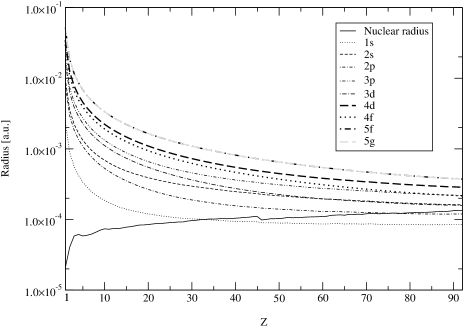
Figure 4: Nuclear radius and average radius of the kaonic atoms levels for $Z=1-92$.

In Figure 4 we plot the nuclear radius and the average radius of some kaonic atoms wavefunction as function of $Z$. This graph shows when the wavefunction radius and the nuclear radius are of the same order of magnitude. It can be used to find which levels are most affected by the strong-interaction for a given $Z$ value.

IV Conclusion

In this work we have evaluated the energies of the circular $(n,\ell=n-1)$, $1\leq n\leq 12$ and first parallel $(n,\ell=n-2)$ levels for several (hydrogenlike) kaonic atoms throughout the periodic table. These energy levels were used to obtain transition energies to compare to the available experimental and theoretical cases.

Our transition energy calculations reproduce experiments on kaonic atoms within the error bar in the majority of the cases. In all the cases the theoretical values are more accurate than experimental ones, as the experiments face the X-ray contamination by other elements.

We have investigated the overlap of the nuclear radius and average radius of kaonic levels as function of $Z$ and the influence of electrons that survived the cascade process on the transition energies.

Table 3: Calculated binding energies of various atomic levels for several kaonic atoms in keV units.

Nucleus	Atomic level	This work	Ref. Iwasaki et al. (1998)	Ref. Baca et al. (2000)
H	$1s$	8.63360	8.634
	$2p$	2.15400	2.154
	$3p$	0.95720	0.957
C	$1s$	430.815		$432\times 10^{0}$
	$2s$	110.579		$111\times 10^{0}$
	$2p$	113.762		$114\times 10^{0}$
Ca	$1s$	3368.58		$344\times 10^{1}$
	$2s$	1042.89		$106\times 10^{1}$
	$2p$	1287.20		$129\times 10^{1}$
	$3p$	573.356		$57\times 10^{1}$
	$3d$	579.932		$58\times 10^{1}$
	$4d$	325.871		$32\times 10^{1}$
Pb	$1s$	17655.61		$1770\times 10^{1}$
	$2s$	9372.797		$939\times 10^{1}$
	$2p$	12749.89		$1277\times 10^{1}$
	$3p$	6830.710		$684\times 10^{1}$
	$3d$	8566.297		$857\times 10^{1}$
	$4d$	4938.662		$494\times 10^{1}$
	$4f$	5471.923		$548\times 10^{1}$
	$5f$	3493.043		$349\times 10^{1}$
	$5g$	3561.058		$356\times 10^{1}$
	$6g$	2471.161		$247\times 10^{1}$
	$6h$	2468.987		$247\times 10^{1}$
	$7h$	1813.611		$182\times 10^{1}$

Table 4: Calculated transition energies and respective contributions, in keV units, for the Al ($5g\rightarrow 4f$) and the Pb ($12o\rightarrow 11n$) transitions. The Al and Pb measured values ($E_{\mbox{m}}$) are from Ref. Bird et al. (1983) and from Ref. Cheng et al. (1975), respectively.

	Al ($5g\rightarrow 4f$)			Pb ($12o\rightarrow 11n$)
	This work	Ref. Barnes et al. (1974)		This work	Ref. Cheng et al. (1975)	Ref. Kunselman (1971)
Coulomb	$49.03755$	49.04		$116.5666$	116.575	116.600
Vacuum Polarization
$\alpha(Z\alpha)$	$0.19048$			$0.4203$	0.421
$\alpha(Z\alpha)^{3}$	$-0.00012$			$-0.0109$	-0.011
$\alpha^{2}(Z\alpha)$	$0.00181$			$0.0040$	0.003
Others					-0.002
Total	$0.19218$	0.19		$0.4135$	0.412	0.410
Recoil	$0.00022$			$0.0004$
Others					-0.044	-0.050
Total	$49.22994$	49.23		$116.9804$	116.943	116.960
$E_{\mbox{m}}$	$49.249(19)$			$116.952(10)$

Table 5: Kaonic atom X-ray energies of circular transitions $(n,\ell=n-1)\rightarrow(n-1,\ell=n-2)$ in keV units. The transitions are identified by the initial ($n_{i}$) and final ($n_{f}$) principal quantum numbers of the atomic levels. The calculated values of the transition energies in this work are compared with the available measured values ($E_{\mbox{m}}$) and with other calculated values ($E_{\mbox{c}}$).

Nucleus	Transition	This work	$E_{\mbox{m}}$	$E_{\mbox{c}}$	Ref.
	$n_{i}\rightarrow n_{f}$
H	$2\rightarrow 1$	6.480	$6.675\ (60)$	$6.482$	Bird et al. (1983)
			$6.96\ (9)$		Izycki et al. (1980)
He	$3\rightarrow 2$	6.463	$6.47\ (5)$	$6.47$	Wiegand and Pehl (1971)
	$4\rightarrow 2$	8.722	$8.65\ (5)$	$8.73$	Wiegand and Pehl (1971)
Li	$3\rightarrow 2$	15.330	$15.320\ (24)$	$15.319$	Batty et al. (1977)
			$15.00\ (30)$	15.28	Berezin et al. (1970)
	$4\rightarrow 2$	20.683	$20.80\ (30)$	$20.63$	Berezin et al. (1970)
Be	$3\rightarrow 2$	27.709	$27.632\ (18)$	$27.632$	Batty et al. (1977)
			$27.50\ (30)$	27.61	Berezin et al. (1970)
	$4\rightarrow 3$	9.677	$9.678\ (1)$	$9.678$	Bird et al. (1983)
C	$4\rightarrow 3$	22.105	$22.30\ (30)$	$22.06$	Berezin et al. (1970)
Al	$4\rightarrow 3$	106.571	$106.45\ (5)$	$106.58$	Barnes et al. (1974)
	$5\rightarrow 4$	49.230	$49.27\ (7)$	$49.23$	Barnes et al. (1974)
			$49.249\ (19)$	49.233	Bird et al. (1983)
	$6\rightarrow 5$	26.707	$26.636\ (28)$	$26.685$	Bird et al. (1983)
	$9\rightarrow 8$	7.151	$7.150\ (1)$	$7.150$	Bird et al. (1983)
Si	$4\rightarrow 3$	123.724	$123.51\ (5)$	$123.75$	Barnes et al. (1974)
	$5\rightarrow 4$	57.150	$57.23\ (7)$	$57.16$	Barnes et al. (1974)
Cl	$4\rightarrow 3$	183.287	$182.41\ (40)$	$183.35$	Kunselman (1971)
	$5\rightarrow 4$	84.648	$84.44\ (26)$	$84.67$	Kunselman (1971)
K	$5\rightarrow 4$	105.952	$105.86\ (28)$	$105.97$	Kunselman (1971)
Ca	$5\rightarrow 4$	117.466	$117.64\ (22)$	$117.48$	Kunselman (1971)
Ti	$5\rightarrow 4$	142.513	$141.8$		Wiegand (1969)
Ni	$5\rightarrow 4$	231.613	$231.49\ (7)$	$231.67$	Barnes et al. (1974)
	$6\rightarrow 5$	125.563	$125.60\ (5)$	$125.59$	Barnes et al. (1974)
	$7\rightarrow 6$	75.606	$75.59\ (5)$	$75.62$	Barnes et al. (1974)
Cu	$5\rightarrow 4$	248.690	$248.50\ (22)$	$248.74$	Barnes et al. (1974)
	$6\rightarrow 5$	134.814	$134.84\ (5)$	$134.84$	Barnes et al. (1974)
	$7\rightarrow 6$	81.173	$81.15\ (5)$	$81.18$	Barnes et al. (1974)
Mo	$8\rightarrow 7$	110.902	$110.90\ (28)$	$110.92$	Kunselman (1971)
Rh	$8\rightarrow 7$	127.392	$127.43\ (31)$	$127.17$	Kunselman (1971)
	$9\rightarrow 8$	87.245	$87.25\ (35)$	$86.66$	Kunselman (1971)
Nd	$9\rightarrow 8$	155.569	$155.60\ (29)$	$155.63$	Kunselman (1971)
	$10\rightarrow 9$	111.159	$110.84\ (32)$	$111.17$	Kunselman (1971)
W	$7\rightarrow 6$	535.240	$534.886\ (92)$	$535.239$	Batty et al. (1989a)
	$8\rightarrow 7$	346.571	$346.624\ (25)$	$346.545$	Batty et al. (1989a)
Pb	$8\rightarrow 7$	426.180	$426.181\ (12)$	$426.201$	Cheng et al. (1975)
			$426.221\ (57)$	426.149	Batty et al. (1989a)
	$9\rightarrow 8$	291.626	$291.577\ (13)$	$291.621$	Cheng et al. (1975)
			$291.74\ (21)$	291.59	Kunselman (1971)
	$10\rightarrow 9$	208.298	$208.256\ (8)$	$208.280$	Cheng et al. (1975)
			$208.69\ (21)$	$208.34$	Kunselman (1971)
	$11\rightarrow 10$	153.944	$153.892\ (11)$	$153.916$	Cheng et al. (1975)
			$154.13\ (21)$	$153.94$	Kunselman (1971)
	$12\rightarrow 11$	116.980	$116.952\ (10)$	$116.943$	Cheng et al. (1975)
			$116.96\ (25)$	$116.96$	Kunselman (1971)
	$13\rightarrow 12$	90.970	$90.929\ (15)$	$90.924$	Cheng et al. (1975)
U	$8\rightarrow 7$	537.442	$538.315\ (100)$	$538.719$	Batty et al. (1989a)

Table 6: Transition energy contributions due to the inclusion of 1, 2, 4 and 10 electrons, in eV units, for Pb ($12o\rightarrow 11n$) and ($13q\rightarrow 12o$) transitions. Effect of the intra-shell correlation $1s^{2}2s^{2}+1s^{2}2p^{2}$ in the Be-like case is presented in the column labeled [Be] corr.

	Transition Energy Contributions
	[H]	[He]	[Be]	[Be] corr.	[Ne]
$12o\rightarrow 11n$	-20.735	-40.917	-47.419	-47.334	-47.484
$13q\rightarrow 12o$	-24.126	-47.609	-55.135	-55.041	-55.245

Table 7: Differences between the measured, $E_{\mbox{m}}$, and the calculated transition energies values, $E$, without electrons and with 1, 2, 3, 4 and 18 electrons, respectively, in eV units. The transitions between ($n$, $\ell=n-1$) states are identified by the initial ($n_{i}$) and final ($n_{f}$) principal quantum numbers of the atomic levels. $\Delta E_{\mbox{m}}$ stands for the experimental uncertainty. For the cases in which there are more than one measure, the weighted average was taken for both $E_{\mbox{m}}$ and $\Delta E_{\mbox{m}}$. In the case of the [Li] core the calculation was made for $J=\ell_{\mbox{kaon}}+1/2$.

	Transition
Nucleus	$n_{i}\rightarrow n_{f}$	$E_{\mbox{m}}-E$						$\Delta E_{\mbox{m}}$	Refs.
		No Elect.	[H]	[He]	[Li]	[Be]	[Ar]
Be	$4\rightarrow 3$	$0.5$	$0.5$	$0.5$	0.5			$1$	Batty et al. (1977)
Al	$9\rightarrow 8$	$-1.0$	$-0.4$	$0$	0.1			$1$	Barnes et al. (1974)
Pb	$8\rightarrow 7$	$-9$	$0$	$8$	$10$	$11$	$12$	$12$	Batty et al. (1989a); Cheng et al. (1975)
	$9\rightarrow 8$	$-49$	$-37$	$-26$	$-25$	$-23$	$-22$	$13$	Kunselman (1971); Cheng et al. (1975)
	$10\rightarrow 9$	$-41$	$-26$	$-12$	$-10$	$-8$	$-7$	$8$	Kunselman (1971); Cheng et al. (1975)
	$11\rightarrow 10$	$-50$	$-33$	$-16$	$-13$	$-10$	$-9$	$11$	Kunselman (1971); Cheng et al. (1975)
	$12\rightarrow 11$	$-27$	$-6$	$14$	$17$	$20$	$22$	$10$	Kunselman (1971); Cheng et al. (1975)
	$13\rightarrow 12$	$-40$	$-10$	$8$	$12$	$15$	$17$	$15$	Kunselman (1971); Cheng et al. (1975)