Relativistic Calculation Of Two-Electron One-Photon And Hypersatellite Transition Energies For $12\leq Z\leq 30$ Elements

Abstract

Energies of two-electron one-photon transitions from initial double K-hole states were computed using the Dirac-Fock model. The transition energies of competing processes, the K$\alpha$ hypersatellites, were also computed. The results are compared to experiment and to other theoretical calculations.

I Introduction

Energies and transition rates for some radiative processes in atoms initially bearing two K-shell holes (two-electron one-photon and one-electron one-photon transitions) were evaluated in this work. This kind of atom, in which an entire inner shell is empty while the outer shells are occupied, was first named hollow by Briand  et al. Briand et al. (1990). Hollow atoms are of great importance for studies of ultrafast dynamics in atoms far from equilibrium and have possible wide-ranging applications in physics, chemistry, biology, and materials science Moribayashi et al. (1998).

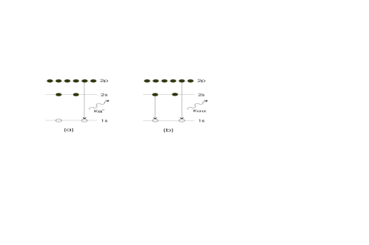
Figure 1: (a) One-electron one-photon transition that produces the K$\alpha^{\text{h}}$ hypersatellite lines; (b) two-electron one-photon transition that produces the K$\alpha\alpha$ lines.

A mono-ionized atom with a K-shell vacancy can decay through an L $\rightarrow$ K electron transition with the emission of x-ray radiation called, in the Siegbahn notation, the K$\alpha$ diagram line. A one-electron transition line for which the initial state has two vacancies in the same shell is called a hypersatellite line. This is the case when a double ionized K-shell state decays through the transition of one L-shell electron (Fig. 1-a), K${}^{-2}\rightarrow$ K^-1L^-1, which is denoted by K$\alpha^{\text{h}}$. A competing, less probable, process of radiative de-excitation from this state is the simultaneous transition of two correlated electrons from higher shells, the K${}^{-2}\rightarrow$ L^-2 transitions, accompanied by the emission of a single photon carrying the total energy, called K$\alpha\alpha$ (Fig. 1-b). Predictions of this decaying process can be found in early papers at the beginning of the twentieth century by Heisenberg Heisenberg (1925) and Condon Condon (1930), but it has only been observed since 1975 Wölfli et al. (1975); Stoller et al. (1977).

For comparison with theory, we should distinguish between experiments in which the initial atomic excitation uses electrons as projectiles  Auerhammer et al. (1988); Salem et al. (1982, 1984), photoionization or nuclear decay  Isozumi (1980), and experiments using heavy ions  Knudson et al. (1976); Wölfli et al. (1975); Stoller et al. (1977). In the latter case, the probability of multiple ionization is usually very high, leading to unreliable determination of energy values. One of the reasons for the scarcity of accurate experimental data stems from the very low intrinsic probability of creating a state with just two K-shell holes.

Theoretical calculations so far have mainly used perturbation theory and were performed in a non-relativistic approach  Gavrila and Hansen (1978); Mukherjee and Mukherjee (1997) with the exception of Chen et al. work  Chen et al. (1982), in which a Dirac-Hartree-Slater approach was used. Indeed, for medium-$Z$ atoms the K-shell electrons are already significantly relativistic, thus calling for relativistic methods in atomic data calculations. In this work we used the Dirac-Fock model to compute transition energies for two-electron one-photon transitions arising from the de-excitation of double 1s hole states leading to final states with two L-shell holes in atoms with $12\leq Z\leq 30$. This is the region of atomic numbers where the transition from the LS to the intermediate coupling scheme occurs. This transition is reflected directly in the K$\alpha^{\text{h }}$ lines relative intensities. We also computed the energies of the competing hypersatellite transitions. The results are compared to experiment and other theoretical calculations.

II Calculation of atomic wave functions and energies

Bound state wave functions and radiative transition probabilities were calculated using the multi-configuration Dirac-Fock program of J. P. Desclaux and P. Indelicato  Desclaux (1975); Indelicato (1996). The program was used in single-configuration mode because correlation was found to be unimportant. The wave functions of the initial and final states were computed independently, that is, atomic orbitals were fully relaxed in the calculation of the wave function for each state, and non-orthogonality was taken in account in transition probabilities calculations.

In order to obtain a correct relationship between many-body methods and quantum electrodynamics (QED) Indelicato (1995); Brown and Ravenhall (1951); Sucher (1980); Mittleman (1981), one should start from the no-pair Hamiltonian

$${\cal H}^{\mbox{{\tiny no pair}}}=\sum_{i=1}^{N}{\cal H}_{D}(r_{i})+\sum_{i<j}{\cal V}(|\bm{r}_{i}-\bm{r}_{j}|),$$ (1)

where ${\cal H}_{D}$ is the one electron Dirac operator and ${\cal V}$ is an operator representing the electron-electron interaction of order one in $\alpha$, properly set up between projection operators $\mathit{\Lambda}_{ij}^{++}=\mathit{\Lambda}_{i}^{+}\mathit{\Lambda}_{j}^{+}$ to avoid coupling positive and negative energy states

$$\mathcal{V}_{ij}=\mathit{\Lambda}_{ij}^{++}V_{ij}\mathit{\Lambda}_{ij}^{++}.$$ (2)

The expression of $V_{ij}$ in the Coulomb gauge and in atomic units is

$$V_{ij}= \,\,\,\,\frac{1}{r_{ij}}$$ (3a)

$$-\frac{\bm{\alpha}_{i}\cdot\bm{\alpha}_{j}}{r_{ij}}$$ (3b)

$$-\frac{\bm{\alpha}_{i}\cdot\bm{\alpha}_{j}}{r_{ij}}[\cos\left(\frac{\omega_{ij}r_{ij}}{c}\right)-1]$$

$$+c^{2}(\bm{\alpha}_{i}\cdot\bm{\nabla}_{i})(\bm{\alpha}_{j}\cdot\bm{\nabla}_{j})\frac{\cos\left(\frac{\omega_{ij}r_{ij}}{c}\right)-1}{\omega_{ij}^{2}r_{ij}},$$ (3c)

where $r_{ij}=\left|\bm{r}_{i}-\bm{r}_{j}\right|$ is the inter-electronic distance, $\omega_{ij}$ is the energy of the photon exchanged between the two electrons, $\bm{\alpha}_{i}$ are the Dirac matrices and $c=1/\alpha$ is the speed of light, $\alpha$ being the fine structure constant. We use the Coulomb gauge as it has been demonstrated that it provides energies free from spurious contributions at the ladder approximation level and must be used in many-body atomic structure calculations Gorceix and Indelicato (1988); Lindroth and Mårtensson-Pendrill (1989).

The term (3a) represents the Coulomb interaction, the term (3b) is the Gaunt (magnetic) interaction, and the last two terms (3c) stand for the retardation operator. In this expression the $\bm{\nabla}$ operators act only on $r_{ij}$ and not on the following wave functions.

By a series expansion of the operators in expressions (3b) and (3c) in powers of $\omega_{ij}r_{ij}/c\ll 1$ one obtains the Breit interaction, which includes the leading retardation contribution of order $1/c^{2}$. The Breit interaction is, then, the sum of the Gaunt interaction (3b) and the Breit retardation

$$B^{\text{\scriptsize{R}}}_{ij}={\frac{\bm{\alpha}_{i}\cdot\bm{\alpha}_{j}}{2r_{ij}}}-\frac{\left(\bm{\alpha}_{i}\cdot\bm{r}_{ij}\right)\left(\bm{\alpha}_{j}\cdot\bm{r}_{ij}\right)}{{2r_{ij}^{3}}}.$$ (4)

In the many-body part of the calculation the electron-electron interaction is described by the sum of the Coulomb and the Breit interactions. Higher orders in $1/c$, deriving from the difference between Eqs. (3c) and (4) are treated here only as a first order perturbation.

All calculations are done for finite nuclei using uniformly charged spheres.

Finally, from a full QED treatment, one also obtains the radiative corrections (important for the innermost shells) to the electron-nucleus interaction (self-energy and vacuum polarization). The one-electron self-energy is evaluated using the one-electron values of Mohr and coworkers  Mohr (1982); Mohr and Kim (1992); Mohr (1992). The self-energy screening is treated with the Welton method developed in Refs. Indelicato et al. (1987); Indelicato and Desclaux (1990); Indelicato and Lindroth (1992); Indelicato et al. (1998). This method yields results in close agreement (better than 5%) with ab initio methods based on QED  Indelicato and Mohr (1991); Blundell (1992, 1993), without the huge amount of effort involved. The vacuum polarization is evaluated as described in Ref. Boucard and Indelicato (2000). The Uelhing contribution is evaluated to all orders by being included in the self-consistent field (SCF). The Wichmann and Kroll and Källén and Sabry contributions are included perturbatively. All three contributions are evaluated using the numerical procedure from Refs. Klarsfeld (1969); Fullerton and G. A. Rinkler (1976).

Breit and QED contributions to the energy of some levels are shown in Table 1 for Mg, Ca and Zn.

III Results

We calculated the energies of the K$\alpha^{\text{h }}$ hypersatellite transitions and the K$\alpha\alpha$ two-electron one-photon transitions for atoms with $12\leq Z\leq 30$.

Depending on the configurations of the initial and final states, for the different values of $Z$, the number of transitions that must be dealt with may range from only two, when the initial state has only closed shells, to several hundred, when unfilled shells exist.

For Mg, Ar, Ca and Zn the 1s^-2 ground configuration corresponds to only one level, the ¹S₀ level, and each of the K$\alpha\alpha$ or K$\alpha^{h}$ lines is identified by a precise level transition,

K$\alpha_{2}\alpha_{3}$:	$1s^{-2\text{ \ }1}$S${}_{0}\rightarrow 2s^{-1}2p^{-1}$ 1P1
K$\alpha_{1}\alpha_{3}$:	$1s^{-2\text{ \ }1}$S${}_{0}\rightarrow 2s^{-1}2p^{-1}$ 3P1
K$\alpha_{2}^{h}$:	$1s^{-2\text{ \ }1}$S${}_{0}\rightarrow 1s^{-1}2p^{-1}$ 1P1
K$\alpha_{1}^{h}$:	$1s^{-2\text{ \ }1}$S${}_{0}\rightarrow 1s^{-1}2p^{-1}$ 3P1

To be able to compare our theoretical transition energy values with experiment and non-relativistic calculations by other authors, we must define the statistical average energy of a line. The energy of all individual $i\rightarrow f$ transitions in the $X$ line, from an initial level $i$, $E_{if}$, weighted by the corresponding transition probability, $W_{if}$, yields the average energy of the $X$ line coming from level $i$, $E_{X}\left(i\right)$:

$$E_{X}\left(i\right)=\dfrac{\sum\limits_{f\left(X\right)}E_{if}W_{if}}{\sum\limits_{f\left(X\right)}W_{if}}$$ (5)

In Eq. (5), $f\left(X\right)$ runs over all possible final levels in the radiative de-excitation leading to the $X$ line, from a specific initial level $i$. Assuming that all states of a $\gamma$ configuration are equally populated, the resulting $E_{X}\left(i\right)$ energies were then weighted by the statistical weight of level $i$, $g\left(i\right)$, leading to the statistical average energy $E_{X}^{\text{SA}}$ for the $X$ line:

$$E_{X}^{\text{SA}}=\dfrac{1}{g\left(\gamma\right)}\sum_{i}g\left(i\right)E_{X}\left(i\right).$$ (6)

Here, ${g\left(\gamma\right)}$ is the statistical weight of the $\gamma$ configuration. We estimate the uncertainty of transition energy values has being of the order of 1 eV.

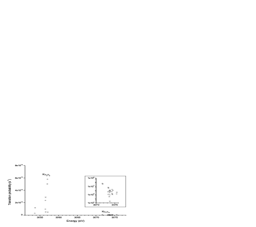
Figure 2: Transition probabilities for all K$\alpha\alpha$ two-electron one-photon transitions in aluminium. The transitions for the initial levels ²P_1/2 and ²P_3/2 are represented, respectively, by $\circ$ and $\times$.

In Table 2, we tabulate the results obtained in this work for the two-electron one-photon radiative transition energies and probabilities from a double K-hole state in aluminium. In this table, the transitions in the K$\alpha\alpha$ lines were ordered by energy: two groups of transitions well separated in energy are clearly identified, which we interpret as being the K$\alpha_{2}\alpha_{3}$ and K$\alpha_{1}\alpha_{3}$ lines, respectively. Further details can be found in Santos et al. (2003). Afterwards, the transitions were grouped, within each of these two groups of transitions, by their initial level, either ²P_1/2 or ²P_3/2. Transition probabilities for all K$\alpha\alpha$ two-electron one-photon transitions in aluminium are shown in Fig. 2.

As can be seen in Table 2, for aluminium the values of the average energy $E_{X}$ for transitions starting from different initial levels are very similar. This is also evident in Table 3, where the average energy values of the x-ray lines for different initial levels of titanium are presented. It is worth mentioning that 401 transition energies were computed to obtain the results corresponding to the K$\alpha\alpha$ lines of the latter case.

To avoid time-consuming calculations, some authors have calculated just the 2s²2p${}^{6}\rightarrow$ 1s²2s2p⁵ transition energy for all values of $Z$, thus neglecting the interaction with the outer electrons. To check the magnitude of the error arising from this simplification, we calculated the transition energies for the atoms with $Z=12,13,18,20,21,22,28,30$, first taking in account all electrons and, in a separate calculation, including in the initial configuration only electrons in the L-shell.

For example, in the case of aluminium K$\alpha\alpha$ lines, we calculated the transition energy for both the 2s²2p⁶3s²3p$\,\rightarrow$1s²2s 2p⁵3s²3p and the 2s²2p${}^{6}\,\rightarrow$1s²2s 2p⁵ transitions. In the particular case of K$\alpha_{2}\alpha_{3}$, we found a 6.8 eV energy difference between the two energy values, out of the 3056.54 eV transition energy (a difference of 0.2 %). Table 4 gives the energy values of the K$\alpha_{2}\alpha_{3}$ line for the 8 elements considered, obtained through the two approaches described. The energy differences, $\Delta E_{\text{th}}$, thus obtained were then fitted to a straight line as a function of $Z$ (Fig. 3). We found that the fit is quite good, presenting a correlation coefficient of 0.998. Using the results of this fitting process, and calculations where only the 2s²2p⁶ electrons were included in the initial states, we obtained K$\alpha_{2}\alpha_{3}$ transition energies for the atoms with the remaining $Z$ values.

Similar behaviour is also observed from the other lines obtained in the decay of a double K-hole state (K$\alpha_{1}\alpha_{3}$, K$\alpha_{2}^{\text{h}}$, K$\alpha_{1}^{\text{h}}$). Thus, using the same method, we were able to obtain the transition energy values for other atoms, with values of $Z$ between 12 and 30, for which complete calculations would involve time-consuming work. For example, for iron ($Z=26$) it would be necessary to calculate around five thousand transition energy values to obtain the energy of the K$\alpha_{2}^{\text{h}}$ and K$\alpha_{1}^{\text{h}}$ hypersatellite or K$\alpha_{2}\alpha_{3}$ and K$\alpha_{1}\alpha_{3}$ lines.

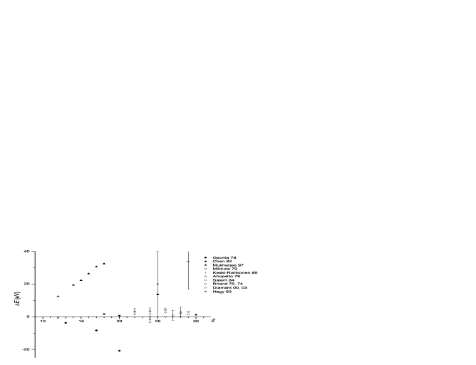
Figure 4: Comparison between available calculated and measured values of K$\alpha_{2}^{\text{h}}$ energy and those of the present work, for $12\leq Z\leq 30$. $\Delta E$ stands for the difference between other energy values and the values obtained in this work.

The results, for all elements with $12\leq Z\leq 30$, are presented in Table  5 and Table  6, where they are compared with other theoretical calculations and experimental values. A comparison between the results of this work for K$\alpha_{2}^{\text{h}}$ line energies and other available results is presented in Fig. 4.

IV Discussion and conclusions

In this work, we computed the energy of K$\alpha_{2}^{\text{h}}$, K$\alpha_{1}^{\text{h}}$, K$\alpha_{2}\alpha_{3}$ and K$\alpha_{1}\alpha_{3}$ lines in the framework of the Dirac-Fock approximation for elements with atomic number $12\leq Z\leq 30$. For selected elements we performed two different calculations: first we took $1$s^-2 as the initial configuration, then we repeated the calculation, considering the 2s²2p⁶ configuration as the initial one. We fitted the differences between the values obtained in the two calculations, as a function of $Z$, to a straight line. We used this result to make a correction to the energies of the remaining elements calculated using the 2s²2p⁶ configuration as the initial one.

These results can be compared with experimental work in which K-holes were obtained using electron bombardment, photo ionization or radioactive decay. Other methods of producing K shell holes, like ion bombardment, will inevitably produce extra holes in the atom, leading to shifts in the measured value of the transition energy, unless the resolution obtained with the detection process is high enough to allow for separation of the peaks resulting from multiple vacancies.

The values obtained in this work for the K$\alpha_{2}^{\text{h}}$ and K$\alpha_{1}^{\text{h}}$ line energies are in excellent agreement with the experimental results (see Fig. 4 for K$\alpha_{2}^{\text{h}}$ energies). We particularly emphasize the agreement with the measured K$\alpha_{2}^{\text{h}}$ energy value of Mikkola et al. Mikkola et al. (1979), for $Z=12$, Keski-Rahkonen et al. Keski-Rahkonen et al. (1985) for $Z=13$, , and Diamant et al. Diamant et al. (2000), for $Z=29$, due to the reported high experimental precision. These authors resolved the x-ray lines using crystal spectrometers.

In Table  5 we present a comparison between our calculated values and the available experimental and theoretical data, in particular those obtained by Chen et al. Chen et al. (1982) in the framework of the Dirac-Hartree-Slater (DHS) method for $Z=18,20,25$ and $30$. The differences between the present calculations and the DHS calculations are probably due mainly to the differences in wave functions (ours were obtained with the optimized level (OL) method and the DHS ones with the configuration-average level method). Additionally, we used an electron-electron operator that avoids coupling between positive and negative states, and we included higher orders in $1/c$ of the Breit interaction.

Our results are closer to experiment than other theoretical results for the K$\alpha_{2}\alpha_{3}$ line; no previous calculation has been reported, to our knowledge, for the K$\alpha_{1}\alpha_{3}$ line. A more detailed comparison with the available experimental results reveals that, for $24\leq Z\leq 29$, our values lie systematically higher (between 0.2% and 0.4%) than the experimental values, outside the reported experimental uncertainty in all cases  Salem et al. (1984); Isozumi (1980). Regarding the value of Auerhammer et al. Auerhammer et al. (1988) for the Al ($Z=13$) K$\alpha_{2}\alpha_{3}$ line, some comments are in order. These authors report the K${}^{-2}\rightarrow$ L^-2 two-electron one-photon lines as well as the K^-2L${}^{-n}\rightarrow$ L^-(2+n) satellite lines, with $n=1,\ldots,4$. They used the calculated values of Tannis et al. Tanis et al. (1977) to propose the identification of most of their measured transition lines. The line with energy difference $\Delta E=E\left(\text{K}\alpha\alpha\right)-2E\left(\text{K}\alpha_{1}\right)=103.4$ eV was labelled by them as the K$\alpha_{2}\alpha_{3}$ line. We suggest that this label should be attributed instead to their unidentified line with energy $\Delta E=84.8$ eV, in much closer agreement with our calculated value $\Delta E=82.2$ eV.

Table 1: QED and Breit contributions to the total energy, $E$, in eV, for Mg, Ca and Zn.

	Mg ($Z$=12)				Ca ($Z$=20)				Zn ($Z$=30)
	1s-2	1s-12p-1	2s-12p-1		1s-2	1s-12p-1	2s-12p-1		1s-2	1s-12p-1	2s-12p-1
	1S0	3P1	3P1		1S0	3P1	3P1		1S0	3P1	3P1
$E$	-2663.734	-4038.075	-5264.540		-10117.187	-14013.573	-17642.276		-29042.059	-37997.033	-46466.031
QED	0.057	0.327	0.549		0.420	1.989	3.311		1.878	8.015	13.235
Breit	0.139	0.249	0.820		1.010	1.822	4.748		4.886	8.158	18.454

Table 2: Two-electron one-photon radiative transition energies ($E_{if}$) and probabilities ($W_{if}$) for the 2s² 2p⁶ 3s² 3p$\rightarrow$1s² 2s 2p⁵ 3s² 3p transition in aluminium. $E_{X}$ is defined by Eq. (5) and $E_{X}^{SA}$ is defined by Eq. (6). Superscripts ^#i are added to distinguish identical terms in the same configuration, where ^#1 stands for the term with the lowest energy. The transtion energy values are in eV.

	Initial Level	Final Level	$E_{if}$	$W_{if}$ (s-1)	$E_{X}$	$E_{X}^{SA}$
K$\alpha_{2}\alpha_{3}$	${}^{2}P_{1/2}$	${}^{2}S_{1/2}$#2	3053.62	2.79$\times 10^{9}$
		${}^{2}P_{3/2}$#2	3056.45	9.53$\times 10^{9}$
		${}^{2}P_{1/2}$#2	3056.47	2.36$\times 10^{10}$
		${}^{2}D_{3/2}$#2	3057.02	5.78$\times 10^{10}$	3056.72
	${}^{2}P_{3/2}$	${}^{2}S_{1/2}$#2	3053.72	1.17$\times 10^{10}$
		${}^{2}P_{3/2}$#2	3056.52	2.87$\times 10^{10}$
		${}^{2}P_{1/2}$#2	3056.54	4.97$\times 10^{9}$
		${}^{2}D_{5/2}$#2	3056.97	5.02$\times 10^{10}$
		${}^{2}D_{3/2}$#2	3057.09	4.69$\times 10^{9}$	3056.45	3056.54
K$\alpha_{1}\alpha_{3}$	${}^{2}P_{1/2}$	${}^{2}S_{1/2}$#1	3071.68	5.06$\times 10^{7}$
		${}^{2}P_{1/2}$#1	3073.19	4.54$\times 10^{5}$
		${}^{2}P_{3/2}$#1	3073.25	1.11$\times 10^{5}$
		${}^{2}D_{3/2}$#1	3073.47	7.41$\times 10^{5}$
		${}^{4}P_{1/2}$	3073.61	2.87$\times 10^{5}$
		${}^{4}P_{3/2}$	3073.65	8.59$\times 10^{4}$
		${}^{4}D_{1/2}$	3074.21	4.77$\times 10^{5}$
		${}^{4}D_{3/2}$	3074.29	1.64$\times 10^{6}$
		${}^{4}S_{3/2}$	3075.50	1.45$\times 10^{5}$	3071.85
	${}^{2}P_{3/2}$	${}^{2}S_{1/2}$#1	3071.75	3.71$\times 10^{7}$
		${}^{2}P_{1/2}$#1	3073.26	5.44$\times 10^{6}$
		${}^{2}P_{3/2}$#1	3073.32	3.78$\times 10^{6}$
		${}^{2}D_{3/2}$#1	3073.54	5.61$\times 10^{4}$
		${}^{4}P_{1/2}$	3073.68	6.84$\times 10^{3}$
		${}^{2}D_{5/2}$#1	3073.69	7.90$\times 10^{5}$
		${}^{4}P_{3/2}$	3073.72	1.17$\times 10^{6}$
		${}^{4}P_{5/2}$	3073.76	6.48$\times 10^{5}$
		${}^{4}D_{1/2}$	3074.28	1.63$\times 10^{5}$
		${}^{4}D_{3/2}$	3074.36	1.12$\times 10^{5}$
		${}^{4}D_{5/2}$	3074.48	9.99$\times 10^{5}$
		${}^{4}S_{1/2}$	3075.57	3.68$\times 10^{5}$	3072.23	3072.10

Table 3: Titanium two-electron one-photon radiative transition average energies in eV of the $X$ line coming from the initial level. $E_{X}^{SA}$ is defined by Eq. (6).

	Initial Level	$E_{X}$	$E_{X}^{SA}$
K$\alpha_{2}\alpha_{3}$	${}^{3}P_{0}$	9144.96
	${}^{1}S_{0}$	9144.93
	${}^{3}P_{1}$	9144.99
	${}^{3}F_{2}$	9144.97
	${}^{1}D_{2}$	9144.97
	${}^{3}P_{2}$	9145.05
	${}^{3}F_{3}$	9145.04
	${}^{3}F_{4}$	9145.12
	${}^{1}G_{4}$	9145.05	9145.04
K$\alpha_{1}\alpha_{3}$	${}^{3}P_{0}$	9174.22
	${}^{1}S_{0}$	9175.64
	${}^{3}P_{1}$	9174.42
	${}^{3}F_{2}$	9173.64
	${}^{1}D_{2}$	9173.98
	${}^{3}P_{2}$	9175.19
	${}^{3}F_{3}$	9174.20
	${}^{3}F_{4}$	9175.37
	${}^{1}G_{4}$	9175.29	9174.72

Table 4: Transition energies in eV for K$\alpha_{2}\alpha_{3}$ calculated using all electrons ($E_{X}^{\text{SA}}$) and using only the 2s² 2p⁶ electrons ($E$*), respectively. $\Delta E_{\text{th}}$ indicates the difference between these energy values: $\Delta E_{\text{th}}$=$E$*-$E_{X}^{\text{SA}}$.

$Z$	Initial Configuration	$E_{X}^{\text{SA}}$	$E$*	$\Delta E_{\text{th}}$
12	2s2 2p6 3s2	2585.45	2589.01	3.56
13	2s2 2p6 3s2 3p	3056.54	3063.37	6.83
18	2s2 2p6 3s2 3p6	6022.29	6056.94	34.65
20	2s2 2p6 3s2 3p6 4s2	7497.79	7546.10	48.31
21	2s2 2p6 3s2 3p6 3d 4s2	8300.74	8353.62	52.88
22	2s2 2p6 3s2 3p6 3d2 4s2	9145.04	9203.25	58.21
28	2s2 2p6 3s2 3p6 3d8 4s2	15098.34	15193.17	94.83
30	2s2 2p6 3s2 3p6 3d10 4s2	17423.97	17533.31	109.34

Table 5: K$\alpha_{2}^{\text{h}}$ and K$\alpha_{1}^{\text{h}}$ theoretical and experimental transition energies in eV. The superscripts stand for: a-Ref. Mikkola et al. (1979), b-Ref. Keski-Rahkonen et al. (1985), c-Ref. Ahopelto et al. (1979), d-Ref. Salem et al. (1984), e-Ref. Briand et al. (1974, 1976), f-Ref. Diamant et al. (2000, 2003) and g-Ref. Nagy and Schupp (1983). Since the K$\alpha_{1,2}^{\text{h}}$ theoretical values obtained by Chen et al. Chen et al. (1982) were presented in the form of energy shifts from the corresponding diagram lines, we used the K$\alpha_{1,2}$ energy values calculated by the same authors Huang et al. (1976) in order to obtain the K$\alpha_{1}^{\text{h}}$ and the K$\alpha_{2}^{\text{h}}$ transition energies. An asterisk indicates that the authors presented experimental results asenergy shifts from the corresponding diagram line. In these cases we took the diagram line energy values from Deslattes et al. (2003).

	K$\alpha_{2}^{\text{h}}$							K$\alpha_{1}^{\text{h}}$
	Theory					Experiment		Theory			Experiment
$Z$	MCDF	Fitted	Ref. Mukherjee and Mukherjee (1997)	Ref. Gavrila and Hansen (1978)	Ref. Chen et al. (1982)			MCDF	Fitted	Ref. Chen et al. (1982)
12	1368.53		1381			1367.8$\pm$0.2${}^{\text{a}}$		1374.34
13	1611.75		1627	1608		1610.8$\pm$0.2${}^{\text{b*}}$		1616.69
14		1874	1893						1880
15		2157	2179						2164
16		2461	2487						2469
17		2785	2816	2777					2794
18	3131.50	3164			3130.9			3141.62		3141.7
19		3498						3508
20	3884.80			3864	3884.4			3896.39		3896.8
21	4294.16							4306.27
22	4723.86					4727$\pm$2${}^{\text{c}}$		4736.76			4741$\pm$3${}^{\text{c}}$
23		5174							5188
24		5647				5650$\pm$2${}^{\text{c}}$			5662		5666$\pm$3${}^{\text{c}}$
						5645$\pm$2${}^{\text{d}}$
25		6140			6140.1	6160$\pm$20${}^{\text{e}}$			6156	6158.0
26		6655		6597		6659$\pm 2^{\text{c}}$			6673		6679$\pm$3${}^{\text{c}}$
						6655$\pm 2^{\text{d}}$					6675$\pm$2${}^{\text{d}}$
						6658$\pm 2^{\text{e*}}$					6677.36$\pm$0.18${}^{\text{f}}$
						6658.31$\pm 0.10^{\text{f}}$
27		7191				7192$\pm 3^{\text{d}}$			7211		7207$\pm$3${}^{\text{d}}$
28	7749.04			7670		7751$\pm 2^{\text{c}}$		7770.90			7775$\pm$3${}^{\text{c}}$
						7752$\pm$3${}^{\text{e*}}$
29		8328				8331$\pm 3^{\text{d}}$			8352		8352$\pm$3${}^{\text{d}}$
						8331$\pm$3${}^{\text{e*}}$					8353.1$\pm$0.7${}^{\text{f}}$
						8329.5$\pm$0.3${}^{\text{f*}}$
						8362$\pm 17^{\text{g}}$
30	8928.53				8928.7			8954.97		8955.4

Table 6: K$\alpha_{2}\alpha_{3}$ and K$\alpha_{1}\alpha_{3}$ theoretical and experimental transition energies in eV. The superscripts stand for: a-Ref. Auerhammer et al. (1988), b-Ref. Salem et al. (1983, 1984) and c-Ref. Isozumi (1980).

	K$\alpha_{2}\alpha_{3}$						K$\alpha_{1}\alpha_{3}$
	Theory				Experiment		Theory		Experiment
$Z$	MCDF	Fitted	Ref. Mukherjee and Mukherjee (1997)	Ref. Gavrila and Hansen (1978)			MCDF	Fitted
12	2585.45		2653				2600.81
13	3056.54		3188	3051	3076.8${}^{\text{a}}$		3072.10
14		3566	3673					3584
15		4118	4240					4137
16		4710	4848					4731
17		5345	5489	5333				5367
18	6022.29		6178				6046.71
19		6378						6764
20	7497.79			7464			7525.09
21	8300.74						8328.97
22	9145.04						9174.72
23		10029						10060
24		10958			10935$\pm$8${}^{\text{b}}$			10990	10960$\pm$8${}^{\text{b}}$
25		11929			11907$\pm$20${}^{\text{c}}$			11962
26		12942		12483	12907$\pm 9^{\text{b}}$			12978	12953$\pm$9${}^{\text{b}}$
27		13999			13945$\pm 10^{\text{b}}$			14036	14005$\pm$10${}^{\text{b}}$
28	15098.34			14960	15060$\pm 10^{\text{b}}$		15136.33		15108$\pm$10${}^{\text{b}}$
29		16240			16193$\pm 10^{\text{b}}$			16281	16236$\pm$10${}^{\text{b}}$
30	17423.97						17466.82

Figure 3: The differences $\Delta E_{\text{th}}$, as a function of atomic number $Z$, between the transition energies calculated for the K$\alpha_{2}\alpha_{3}$ line, using only the 2s² 2p⁶ configuration and using the 1s^-2 configuration (+). The straight line represents the linear regression to these energy differences.