Chirality Selection Models in a Closed System

Abstract

Recently the first chemical systems which show the amplification of enantiomeric excess (ee) was found. Inspired by these experiments, we propose a few chemical reaction models in a closed system. The reactions consist of autocatalytic production of chiral molecules and their decomposition processes. By means of flow diagrams in the phase space of enatiometric concentrations, chiral symmetry breaking is studied.

Without any destruction processes, the quadratic autocatalysis leads to the amplification of ee, but the flow is attracted to a fixed line, which is only marginally stable. The destruction processes alter the attractor structure completely. With a cross inhibition the linear autocatalysis is sufficient for the chiral symmetry breaking with a complete homochirality. With a back reaction, the quadratic autocatalysis is necessary to bring about the chiral symmetry breaking. The final ee is not complete if there is a racemization process.

I Introduction

Because of the three-dimensional tetragonal arrangement of four chemical bonds around a carbon atom, organic molecules can take two types of stereostructures; a right-handed one and a mirror-image left-handed one. bonner88 ; feringa+99 The molecules which have either of these two forms are called chiral, and the two forms are enantiomers with each other. In general the two types are classified in $R$ and $S$ forms, but, for sugars and amino acids, D and L representations are common in use. From energetic point of view, the two enantiomers are indistinguishable and they should exist with equal probability. In fact, in the usual chemical reactions both types of enatiomers are produced with equal probabilities, and the product is called a racemate or a racemic mixture.

In contrast, life on earth utilizes only one type of enantiomers: levorotatory(L)-amino acids and dextrorotatory(D)-sugars. This symmetry breaking in chirality is called the homochirality, and the origin of this unique chirality selection has long been intriguing many scientists. bonner88 Various mechanisms have been proposed to induce an asymmetry in the primordial molecular environment, mason+85 ; kondepudi+85 ; meiring87 ; bada95 ; bailey+98 ; feringa+99 ; hazen+01 but the induced chiral asymmetry in all the proposed models is expected to be very minute. Therefore, the mechanisms to amplify enormously the enatiometric excess (ee) are indispensable.

Frank is the first to show that an autocatalytic chemical reaction with an antagonistic process in open systems can lead to an amplification of ee.frank53 Many theoretical models have since been proposed, but they are often criticized as lacking any experimental support. bonner88 Recently, a first system which shows the spontaneous amplification of ee has been found by Soai’s group. soai+90 ; soai+95 ; sato+01 ; sato+03 This enhancement takes place in a closed system, and is explained by the second-order autocatalytic reaction.sato+03 Inspired by these experiments, soai+90 ; soai+95 ; sato+01 ; sato+03 we constructed some simple models of autocatalytic chemical reactions in a closed and conserved system, saito+04a ; saito+04b and studied conditions when the chiral symmetry breaking is possible. Here we extend these models and study them in detail.

In §2, we summarize the fundamental aspects of autocatalytic reaction models where two enantiomers compete against each other in a closed system for the limited resource.saito+04a The ee amplification is found possible if the production of chiral molecules contains the quadratic autocatalytic process. However, concentrations of enantiomers are attracted to a fixed line, which is only marginally stable. Therefore, the final configuration might be susceptible to external perturbation. In §3, with the mutual antagonism or the cross inhibition, the complete homochirality is concluded if there is a linear autocatalysis. In §4, with the back reaction, the quadratic autocatalysis is found necessary for the chirality selection. Summary and discussions are given in the last section §5.

II Autocatalytic Reactions in a Closed System

We start our study about reaction models with autocatalytic productions of chiral molecules from achiral materials. Frank frank53 has considered the chiral symmetry breaking in an open chemical system. However, since the experiment is performed in a closed system, soai+95 we consider reaction models in a closed and conserved system, and explore effects that the autocatalysis alone can lead.

Suppose two achiral molecules A and B react to produce a chiral molecule C. For the purpose of simplicity we denote ($R$)-C molecule as R and ($S$)-C molecule as S, hereafter. The reactions A+B$\rightarrow$ R and A+B$\rightarrow$ S proceed in a closed system, and thus they stop when the materials A and/or B are exhausted. Here we assume that there is an ample amount of material B, and its concentration can be regarded as constant all through the reaction. Then, the process depends only on the concentrations of A, R and S molecules, which we denote $a,~{}r$ and $s$, respectively. The conservation of the total number of participating molecules gives the relation that the total concentration stays constant determined by the initial values as

$$a+r+s=a_{0}+r_{0}+s_{0}=c_{0}=\mbox{const.}$$ (1)

Then the reaction developement can be depicted as a flow in the $r$-$s$ phase diagram. The conservation law (1) limits the phase space in the triangular region

$$0\leq r,s\leq c_{0},\quad 0\leq r+s\leq c_{0}.$$ (2)

As a first step we consider the simplest autocatalytic reaction model such that the production from the material A to R or S is described by the following rate equations:

$$\frac{dr}{dt}=f(r)a=f(r)(c_{0}-r-s)$$

$$\frac{ds}{dt}=f(s)a=f(s)(c_{0}-r-s)$$ (3)

with

$$f(x)=k_{0}+k_{1}x+k_{2}x^{2}.$$ (4)

The coefficient $k_{0}$ represents the rate of a nonautocatalitic reaction, $k_{1}$ of a linearly autocatalytic and $k_{2}$ of a quadratically autocatalytic reactions. Since all the rates $k_{0,1,2}$ are non-negative, $f(x)\geq 0$ for $x=r$ and $s$. In the Soai reaction, the quadratic autocatalysis is shown to explain the time evolution of the reaction yield and the ee.sato+03

II.1 Fixed points

We now study the flow diagram in $r-s$ space in typical situations. First we search fixed points of Eq.(3) in the region (2). It is easy to find that $a=0$ gives a line of fixed points at $r+s=c_{0}$, which are stable and correspond to the state where all the material A is consummed up. Only for the case without nonautocatalysis, $k_{0}=0$, another fixed point is possible at the origin $r=s=0$, but it is easily shown to be unstable.

Figure 1: Flow diagrams for (a) nonautocatalytic ($k_{0}>0,~{}k_{1}=k_{2}=0$), (b) linearly autocatalytic ($k_{1}>0,~{}k_{0}=k_{2}=0$), and (c) quadratically autocatalytic ($k_{2}>0,~{}k_{0}=k_{1}=0$) reactions.

The flow will then be attracted to the fixed line $r+s=c_{0}$, and is given by the equation

$$\int\frac{dr}{f(r)}-\int\frac{ds}{f(s)}=\mathrm{constant}.$$ (5)

Integration of this equation for general $f(x)$ can be carried out analytically, but we discuss the flow lines only in three typical cases in the following.
$\bullet$ Nonautocatalytic case:

Without autocatalysis, $k_{0}>0$ but $k_{1}=k_{2}=0$, flow lines are easily obtained by interation of eq.(5) and they have a unit slope, $r-s=r_{0}-s_{0}=$constant, as shown in Fig.1(a).
$\bullet$ Linearly autocatalitic case:

With only a linear autocatalysis, $k_{1}>0,~{}k_{0}=k_{2}=0$, the integration of eq.(5) is easy to yield the trajectory $r/s=r_{0}/s_{0}=$constant. The flow is represented by lines projecting out from the origin, as shown in Fig.1(b).
$\bullet$ Quadratically autocatalytic case:

For a quadratically autocatalytic case, $k_{2}>0,~{}k_{0}=k_{1}=0$, flow lines are a collection of hyperbolae projecting out from the origin, $1/r-1/s=1/r_{0}-1/s_{0}=$constant, as shown in Fig.1(c).

II.2 Enatiometric Excess

In order to quantify the ee or the degree of chiral symmetry breaking, we use an order parameter $\phi$ defined as

$$\phi=\frac{r-s}{r+s}.$$ (6)

$\bullet$ Nonautocatalytic case:

For the non-autocatalytic case in Fig.1(a), the numerator $r-s$ remains constant during the time evolution whereas the denominator $r+s$ increases. Thus the ee decreases monotonously from the initial value $|\phi_{0}|=|(r_{0}-s_{0})/(r_{0}+s_{0})|$ to the asymptotic one $|\phi_{\infty}|=|(r_{0}-s_{0})/c_{0}|$. If the initial concentrations $r_{0}$ and $s_{0}$ are small, ee $|\phi|$ becomes very small. This result is quite natural from the microscopic point of view, since the nonautocatalytic reaction produces both enatiomers randomly and leads to the racemization.
$\bullet$ Linearly autocatalytic case:

For the linearly autocatalytic case in Fig.1(b), the ratio $r/s$ remains constant and so does the ee.
$\bullet$ Quadratically autocatalytic case:

Only with a nonlinear autocatalysis in Fig.1(c), the ee increases up to some saturation value $|\phi_{\infty}|$, as shown in Fig.2. This asymptotic value of $\phi_{\infty}$ depends on the initial concentrations $r_{0}$ and $s_{0}$, even when the initial $\phi_{0}$ and the total $c_{0}$ are fixed, as shown in Fig.2. The smaller the initial amount of chiral molecules ($r_{0}+s_{0}$) are, the more the ee is amplified.

Figure 2: Time evolution of the enantiomeric excess $\phi$ with quadratic autocatalytic reaction $k_{2}>0$ with the same initial value $\phi_{0}$ but the different amount of initial R and S molecules, $r_{0}$ and $s_{0}$.

$\bullet$ General case:

For more general cases, the ee amplification is explained by studying the evolution of $\phi$, which is derived from eq.(3) as

$$\frac{d\phi}{dt}=\frac{a}{c_{0}-a}\phi[-2k_{0}+\frac{k_{2}}{2}(c_{0}-a)^{2}(1-\phi^{2})].$$ (7)

The evolution equation turns out to be independent of the linear autocatalytic rate $k_{1}$. Without quadratic autocatalysis ($k_{2}=0$) the ee decreases as we have already observed, since the concentration of A material, $a$, and the sum of R and S products, $c_{0}-a=r+s$, should always be positive. The situation does not alter by including only a linear autocatalysis with $k_{1}>0$: it does not directly affect the evolution of $\phi$. Only when the quadratic auatocatalysis dominates at $k_{2}>4k_{0}/c_{0}^{2}$, the ee can increase. Therefore, in this simplest model only the quadratic autocatalysis can enhance the chiral assymmetry. This may correspond to the situation observed in the Soai reaction. It has to be noted that the asymptotic value $\phi_{\infty}$ cannot be determined from eq.(7), since $\displaystyle\lim_{t\rightarrow\infty}a(t)=0$ in the present model.

Even though the amplification of the enatiometric excess or the amplification of the chiral assymmetry can be brought about by the nonlinear autocatalysis, the final state of the system is on the line of fixed points, and thus the final values of ee can be anything depending on the initial condition. Since these points are marginally stable, i.e. they have no quaranteed stability along the direction of the fixed line, they may be susceptible to additional perturbations. We now consider the effect of two types of destructive reactions of chiral molecules.

III With Cross Inhibition

Frank has introduced the mutual antagonism between the enantiomers, R and S, and succeeded in explaining the chiral symmetry breaking in an open reaction system. Here we extend his model to the closed system. The reaction equation now incorporates terms of cross inhibition as

$$\frac{dr}{dt}=f(r)a-\mu rs$$

$$\frac{ds}{dt}=f(s)a-\mu rs.$$ (8)

III.1 Fixed points

Fixed points have to satisfy the relation

$$f(r)a=f(s)a=\mu rs.$$ (9)

The simplest solution is $a=0$ and $rs=0$, which corresponds to the end corners of the triangular region, $(r,~{}s)=(c_{0},~{}0)$ and $(0,~{}c_{0})$. These are easily shown to be stable with complete homochirality, $\phi=\pm 1$. Other fixed points are also possible with a nonzero $a$ and $f(r)=f(s)=\mu rs/a$. We shall study them in various cases below.
$\bullet$ Nonautocatalytic case:

Only with a nonautocatalytic reaction ($k_{0}>0,~{}k_{1}=k_{2}=0$), $f(r)=f(s)=k_{0}$ and there is a fixed line

$$\displaystyle{(r+\frac{k_{0}}{\mu})(s+\frac{k_{0}}{\mu})=\frac{k_{0}}{\mu}(c_{0}+\frac{k_{0}}{\mu})}$$ (10)

passing through the two terminal points $(r,~{}s)=(c_{0},~{}0)$ and $(0,~{}c_{0})$. This line is an accumulation of infinitely many marginal fixed points. In fact the flow trajectory is easily integrated as $r-s=r_{0}-s_{0}=$constant, the same lines with a unit slope obtained in the previous section without cross inhibition. The cross inhibition only shifts the fixed line from the border $r+s=c_{0}$ in Fig.1(a) to the hyperbola (10).

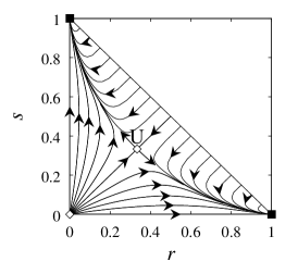
Figure 3: Flow diagrams with cross inhibition $\mu c_{0}=1$ at (a) $k_{0}>0,~{}k_{1}=k_{2}=0$ and (b) $k_{1}>0,~{}k_{0}=k_{2}=0$.

$\bullet$ Linearly autocatalytic case:

With a finite $k_{1}$ as well as $k_{0}$, a fixed line is replaced by a symmetric fixed point U at

$$r=s=\frac{-2k_{0}+k_{1}c_{0}+\sqrt{(2k_{0}+k_{1}c_{0})^{2}+4k_{0}c_{0}\mu}}{2(\mu+2k_{1})}.$$ (11)

At $k_{0}=0$, there appears an additional fixed point at the origin $r=s=0$. All these fixed points are easily shown to be unstable, as shown in Fig.3(b). The only stable fixed points are those at the corners, $(c_{0},0)$ and $(0,c_{0})$, with the complete homochirality. Thus, with only a linear autocatalysis and without any nonlinear ones, complete homochirality is possible with a cross inhibition even in a closed system.

With quadratic autocatalysis, the overall structure of the flow is similar to the case with a linear autocatalysis.

III.2 Enantiomeric excess

Up to the linear autocatalysis ($k_{2}=0$) with a cross inhibition ($\mu\neq 0$), the ee follows the evolution equation

$$\frac{d\phi}{dt}=\frac{1}{c_{0}-a}\phi[-2k_{0}a+\frac{\mu}{2}(c_{0}-a)^{2}(1-\phi^{2})].$$ (12)

The rate $k_{1}$ of the linear autocatalytic process is not involved in the symmetry breaking effect of $\phi$ neither in the present case with cross inhibition nor in the case without cross inhibition in the previous section. One notices the similarity between the evolution equation (12) and eq.(7) derived in the previous section. The effect of the quadratic autocatalytic reaction, $k_{2}$, in eq.(7) is replaced by $\mu/a$ in eq.(12). In the present case, the symmetry recovering effect $k_{0}$ weakens as the material A is consumed ($a\rightarrow 0$), and the complete homochirality $\phi=\pm 1$ is achieved asymptotically. For example, the time evolution of $r/c_{0},~{}s/c_{0}$ and $\phi$ is depicted in Fig.4 at $k_{0}=0,k_{1}c_{0}=1,\mu c_{0}=1$ and $r_{0}/c_{0}=0.0714,s_{0}/c_{0}=0.0700,\phi_{0}=0.01$. Initially $r$ and $s$ increase simultaneously to approach the symmetric fixed point U: $(r/c_{0},~{}s/c_{0})$=(1/3,1/3) with a constant $\phi\approx\phi_{0}$, driven by the linear autocatalytic process $k_{1}$. However, since U is unstable, the trajectory is eventually expelled from U and $r$ increases at the cost of $s$. As a result $\phi$ increases to the full homochirality.

Figure 4: Time evolution of $r,s$, and $\phi$ at $k_{0}=0,k_{1}c_{0}=1,\mu c_{0}=1$ and $r_{0}/c_{0}=0.0714,s_{0}/c_{0}=0.0700,\phi_{0}=0.01$.

IV With Back Reactions

We now consider another type of decomposition process, a simple back reaction from the product R or S to an A molecule. Governing equations are

$$\dot{r} =f(r)a-\lambda r$$

$$\dot{s} =f(s)a-\lambda s$$ (13)

Since the back reaction is linear in the product concentrations $r$ and $s$, the evolution of the ee remains the same with eq.(7). Therefore, the quadratic autocatalysis with a finite $k_{2}$ is the necessity to break the chiral symmetry in the present case. Even though $\phi$ follows the same evolution (7) without the back reaction, its asmptotic behavior is quite different from that in §2, because the fixed point structure is drastically altered by the back reaction.

Fixed points

Fixed points of the flow satisfy conditions

$$f(r)a-\lambda r=f(s)a-\lambda s=0.$$ (14)

It is trivial that $a=0$ cannot be a fixed point any more unless $c_{0}=0$. As we have supposed, the fixed line $r+s=c_{0}$ in §2 is very sensible to the perturbation like a back reaction. We now study structures of fixed points in some simple cases.

$\bullet$ Nonautocatalytic case:

In the non-autocatalytic case with $k_{0}>0,~{}k_{1}=k_{2}=0$ with a finite $\lambda$, there is only a symmetric fixed point at

$$r=s=\frac{c_{0}/2}{1+\lambda/2k_{0}}~{}<~{}\frac{c_{0}}{2},$$ (15)

which is easily shown to be stable, as shown in Fig.5(a).

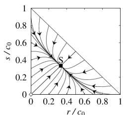
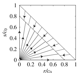
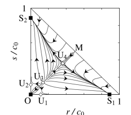
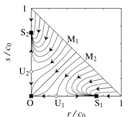
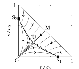
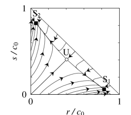
Figure 5: Flow diagrams for (a) $k_{0}>0,~{}k_{1}=k_{2}=0,\lambda=1$, (b) $k_{1}=1,k_{0}=k_{2}=0,\lambda=0.1$, (c) $k_{2}=1,~{}k_{0}=k_{1}=0,\lambda=0.1$, (d) $k_{2}=1,~{}k_{0}=k_{2}=0,\lambda=0.2$, (e) $k_{1}c_{0}=0.4,k_{2}c_{0}^{2}=1,~{}k_{0}=0,\lambda=0.3$. (f) $k_{0}=0.05,k_{1}c_{0}=0.,k_{2}c_{0}^{2}=1,\lambda=0.1$.

Figure 6: Time evolution of the ee $\phi$ with nonlinear autocatalysis and a back reaction (a) without random creation $k_{0}=0$, and (b) with a finte $k_{0}=0.05$.

$\bullet$ Linearly autocatalytic case:

With only a linear autocatalysis $k_{1}>0,~{}k_{0}=k_{2}=0$, we have only a trivial fixed point at the origin $(r,s)=(0,0)$, when the rate of back reaction is as large as $\lambda\geq k_{1}c_{0}$: there will be no net production of chiral C molecules because of strong back reaction. On the contrary, when the rate of back reaction is small as $\lambda<k_{1}c_{0}$, there are additional fixed points on a line $r+s=c_{0}-\lambda/k_{1}$. This line corresponds to the one $r+s=c_{0}$ in §2 shifted by the back reaction $\lambda$. In fact the trajectory is the same as in §2 and radiates from the origin $r/s=r_{0}/s_{0}=$constant, as shown in Fig.5(b).

$\bullet$ Quadratically autocatalytic case:

With a quadratic autocatalysis $k_{2}>0,k_{0}=k_{1}=0$, the back reaction decimates the fixed line $r+s=c_{0}$ and produces several fixed points. One of them is a trivial fixed point at the origin $(r,s)=(0,0)$, which is of no interest.

1. With a small rate of back reaction, $\lambda<k_{2}c_{0}^{2}/8$, there are other six fixed points: two on the $r$ axis, U${}_{1}:~{}(A_{-},0)$ and S${}_{1}:~{}(A_{+},0)$, two on the $s$ axis, U${}_{2}:~{}(0,A_{-})$ and S${}_{2}:~{}(0,A_{+})$, and two symmetric ones, U${}_{3}:~{}(B_{-},B_{-})$ and U${}_{4}:~{}(B_{+},B_{+})$, with

   $$A_{\pm} =\frac{c_{0}}{2}\left(1\pm\sqrt{1-\frac{4\lambda}{k_{2}c_{0}^{2}}}\right)$$

   $$B_{\pm} =\frac{c_{0}}{4}\left(1\pm\sqrt{1-\frac{8\lambda}{k_{2}c_{0}^{2}}}\right).$$

   As an illustration shown in Fig.5(c), we use parameter values $k_{2}c_{0}^{2}=1,~{}\lambda=0.1$, which gives fixed points U_1-4 and S_1,2 specified by the values, $A_{+}=0.8873c_{0}=c_{0}-A_{-}$, and $B_{+}=0.3618c_{0}=c_{0}/2-B_{-}$. The stable fixed points S₁ and S₂ correspond to the states with complete homochirality with $\phi=\pm 1$. Except the region around the trivial fixed point O, the phase flow is attracted to one of these two homochiral states, S₁ or S₂. Generally, the region of initial points which will eventually be attracted to a certain fixed point is called the basin of attraction. In the present case, the $r-s$ phase space is divided into three basins of attractions to S₁, S₂, and O, by separatrixes U₃U₁, U₃U₂, and U₃M.

   The time evolution of the order parameter $\phi$ is depicted in Fig.6(a) with the parameters $k_{0}=k_{1}=0,k_{2}c_{0}^{2}=1,\lambda c_{0}=0.1$, the same ones used to obtain the flow diagram in Fig.5(c). The initial condition is $r_{0}=0.2+0.001,s_{0}=0.2$. The flow is almost symmetric as $r\approx s$ first and approaches to the symmetric fixed point U₄, but since U₄ is unstable $r$ starts to increase at the cost of $s$ and eventually $\phi$ approaches the full value, unity.

2. As the back reaction rate increases, two symmetric fixed points U₃ and U₄ merge to disappear for $\lambda\geq k_{2}c_{0}^{2}/4$. There remains two homochiral fixed points S₁ and S₂. Their basins of attraction are close to the $r$ or $s$ axes. Close to the diagonal $r=s$ the flow runs to the trivial fixed point O. The separatrixes of three basins of attractions are U₁M₁ and U₂M₂. With the parameter values $k_{2}c_{0}^{2}=1,~{}\lambda=0.2$, fixed points S₁ and S₂ are determined with parameters $A_{+}=0.7236c_{0}$ and $A_{-}=c_{0}-A_{+}$, as shown in Fig.5(d).

3. Finally, when the back reaction is too strong as $\lambda\geq k_{2}c_{0}^{2}/4$, all the flow runs to the origin.

$\bullet$ Linear and quadratic autocatalysis:

We consider now the effect of a linear autocatalytic process in addition to the quadratic autocatalysis $k_{2}$. As far as $k_{1}$ is smaller than $\lambda/c_{0}$, the origin $r=s=0$ is attractive, and the schematics of the flow in the $r-s$ phase space is the same with those for $k_{1}=0$. When $k_{1}$ is larger than $\lambda/c_{0}$, the origin $r=s=0$ looses the stability, and there are only three fixed points: two stable ones on $r$ and $s$ axes S₁: $(C,0)$ and S₂: $(0,C)$ and a symmetric and unstable one at U: $(D,D)$ with

$$C =\frac{k_{2}c_{0}-k_{1}+\sqrt{(k_{2}c_{0}+k_{1})^{2}-4k_{2}\lambda}}{2k_{2}}$$

$$D =\frac{k_{2}c_{0}-2k_{1}+\sqrt{(k_{2}c_{0}+2k_{1})^{2}-8k_{2}\lambda}}{4k_{2}}.$$

and the typical flow in this case with $k_{0}=0,k_{1}c_{0}=0.4,k_{2}c_{0}^{2}=1,\lambda=0.3$ is shown in Fig.5(e), which looks similar to the case with the cross inhibition shown in Fig. 3(b): complete homochiral states, $\phi=\pm 1$, is attained asymptotically even though not all the A material is consumed.

$\bullet$ Autocatalysis with nonautocatalytic production

We found that the quadratic autocatalysis with back reaction permits to attain the homochiral situation, if there are a few C molecules initially outside the basin of attractive to the origin $r=s=0$. In order to actuate the autocatalysis, however, one has to provide initial C molecules. Therefore, nonautocatalytic production with a finite $k_{0}$ seems necessary. We now consider cases when the random creation of racemic mixtures by $k_{0}$ coexist with the autocatalytic production as well as the back reaction.

1. With a linear autocatalysis $k_{0}>0,~{}k_{1}>0,k_{2}=0,\lambda>0$, the fixed line for $k_{0}=0$ in Fig.5(b) is replaced by a symmetric fixed point at

   $$r=s= \frac{1}{4k_{1}}\Big{\{}k_{1}c_{0}-2k_{0}-\lambda$$

   $$+\sqrt{(k_{1}c_{0}-2k_{0}-\lambda)^{2}+8k_{0}k_{1}c_{0})}\Big{\}}$$ (16)

   which is stable and $\phi=0$. Random racemization effect by $k_{0}$ dominates and recovers the symmetric state.

2. With a quadratic autocatalysis $k_{0}>0,~{}k_{2}>0,~{}k_{1}=0$, the situation is rather complex. Since $f(0)\neq 0$, all the fixed points stay within the triangle (2); $a,~{}r,~{}s\neq 0$. Then the fixed points satisfy the relation

   $$\frac{k_{0}+k_{2}r^{2}}{r} =\frac{\lambda}{a}=\frac{k_{0}+k_{2}s^{2}}{s}$$

   $$\rightarrow~{}~{}(r-s)(k_{0}-k_{2}rs)=0$$ (17)

   The symmetry broken states stay on a hyperbola $rs=k_{0}/k_{2}$. They satisfy further the relation

   $$\Lambda_{a}(r) \equiv k_{2}\left[\frac{c_{0}^{2}}{4}-\left(r-\frac{c_{0}}{2}+\frac{k_{0}}{k_{2}r}\right)^{2}\right]$$

   $$=\lambda>0.$$ (18)

   If $k_{0}$ is smaller than $k_{2}c_{0}^{2}/16$, the function $\Lambda_{a}(r)$ in eq.(18) has two peaks with a height $\lambda_{\mathrm{m}ax}=k_{2}c_{0}^{2}/4$, as shown in Fig.7(a). It also has a local minimum value $\lambda_{\mathrm{m}in}=2\sqrt{k_{0}}(c_{0}\sqrt{k_{2}}-2\sqrt{k_{0}})$ at $r=\sqrt{k_{0}/k_{2}}$. Then for small $\lambda<\lambda_{\mathrm{m}in}$ there are two solutions of asymmetric fixed points which are stable, for intermediate case with $\lambda_{\mathrm{m}in}<\lambda<\lambda_{\mathrm{m}ax}$ there are four solutions two among them are stable and two other are unstable, and for large $\lambda>\lambda_{\mathrm{m}ax}$ there is none.

   If $k_{0}$ lies between $k_{2}c_{0}^{2}/16$ and $k_{2}c_{0}^{2}/4$, $\Lambda_{a}(r)$ has only a single peak with a value $\lambda_{\mathrm{m}ax}^{\prime}=2\sqrt{k_{0}}(c_{0}\sqrt{k_{2}}-2\sqrt{k_{0}})$. Therefore the number of solutions are two for small $\lambda<\lambda_{\mathrm{m}in}^{\prime}$ which are stable, and none for large $\lambda$.

   Further larger $k_{0}>k_{2}c_{0}^{2}/4$, there is no asymmetric fixed point for any $\lambda$. The last result is already drawn by the time evolution of $\phi$ given in Eq.(7), which is valid in the present case, too.

   

   

   Figure 7: Functions (a) $\Lambda_{a}(r)$ and (b) $\Lambda_{s}(r)$ to determine (a) asymmetric and (b) symmetric fixed points.

   As for the symmetric solutions with $r=s$, the effect of random creation $k_{0}$ is more effective. Since the fixed points have to satisfy a relation

   $$\Lambda_{s}(r)\equiv \frac{k_{2}c_{0}^{3}}{r}\Big{[}-2\Big{(}\frac{r}{c_{0}}-\frac{1}{6}\Big{)}^{3}$$

   $$+\Big{(}\frac{k_{0}}{k_{2}c_{0}^{2}}-\frac{1}{108}\Big{)}\Big{]}+2\Big{(}\frac{k_{2}c_{0}^{2}}{12}-k_{0}\Big{)}$$

   $$= \lambda,$$ (19)

   the number of fixed points reduces to one which is unstable if $k_{0}$ is larger than $k_{2}c_{0}^{2}/108$, as shown in Fig.7(b). For a small rate $k_{0}\leq k_{2}c_{0}^{2}/108$, the numbers of symmetric fixed points depends on $\lambda$. For a small $\lambda$, there is one unstable, for an intermediate value of $\lambda$ there are three among which one is stable and two unstable, and for a large $\lambda$ there remains only one stable one. For example, by adding $k_{0}$ as small as $k_{0}=0.05(>k_{2}c_{0}^{2}/108)$ to the situation shown in Fig.5(c), the origin looses the stability and there remains only a single symmetric fixed point which is unstable. Therefore, the flow diagram reduces to the one shown in Fig.5(f). The achieved ee is not complete, but is very large if $k_{0}$ is small, as shown in Fig.6(b). There the initial condition is chosen as $r_{0}=0.1+0.001$ and $s=0.1$, but the final $\phi$ deos not depend on the initial values of $r_{0}$ or $s_{0}$.

V Summary and Discussions

We studied various autocatalytic models with back reaction or with cross inhibition processes to search for the conditions to achieve the chirality selection in a closed system. The results are summarized in the Table 1.

	$k_{0}$	$k_{1}$	$k_{2}$	$\lambda$	$\mu$	SB	section
(1)	$\geq$	$\geq$	$\geq$	$0$	$0$	S	§2
(2)	$\geq$	$0$	$0$	$0$	$>$	S	§3
(3)	$\geq$	$>$	$\geq$	$0$	$>$	B	§3
(4)	$\geq$	$\geq$	$0$	$>$	$0$	S	§4
(5)	$\geq$	$\geq$	$>$	$>$	$0$	B	§4
$\dot{r}=(k_{0}+k_{1}r+k_{2}r^{2})a-\lambda r-\mu rs$
$\dot{s}=(k_{0}+k_{1}s+k_{2}s^{2})a-\lambda s-\mu rs$
$a=c_{0}-r-s$

Table 1: Classification of reaction models with parameters defined in the bottom column. Symbol $\geq$ means that the value is non-negative and $>$ means that the value must be positive. B means that the final state is chiral symmetry breaking and S means otherwise. Details for each entry are explained in the indicated sections.

If the production of chiral molecules R and S from the achiral material A involves a linear autocatalysis, the cross inhibition between R and S is necessary to realise the homochirality, as is summarized for the cases (1)-(4) in Table 1. The case (3) corresponds to an extension of Frank’s model to a closed chemical system.

With a quadratic autocatalysis, the amplification of enantiomeric excess (ee) is achieved without any destruction process, but the steady state can have any finite value of ee ($-1\leq\phi\leq 1$), as the stable fixed line exists extending from $\phi=1$ to $\phi=-1$. In fact the final value of ee depends on the details of the initial values of chiral as well as achiral materials’ concentrations. Therefore we do not regard this case (1) as the chiral symmetry breaking in a restricted sense.

With a linear back reaction process and a quadratic autocatalysis as a special case of (5), the complete homochirality is possible to realize when the rate of back reaction is sufficiently small. The minority enantiomer is decomposed back to the material A and recycled to produce the majority enantiomer and vice versa. This decomposition process works more effectively for the minority because of the suppressed production due to the nonlinear autoctalysis.

However, with only autocatalytic processes, the initial production of chiral molecules is impossible. Therefore, the random production of chiral molecules by the nonautocatalytic process described by a nonzero value of coefficent $k_{0}$ is indispensable. For a small value of $k_{0}$, the phase space structure of the flow and fixed points is not qualitatively affected and resembles with that of vanishing $k_{0}$ case. However, for $k_{0}$ greater than the critical value $k_{2}c_{0}^{2}/108$, this process affects the structure of racemic fixed points so drastically that the system can have only almost homochiral states as stable fixed points, as shown in Fig.5(f).

We have studied two types of simple models (3) and (5) where the chiral symmetry can be broken in the closed system and complete or almost complete homochiral states can be achieved. One type of the model with the cross inhibition (3) seems powerful for this purpose, but the chemical system which shows this process has not been found so far and it is very interesting to find actual chemical system. On the other hand, the nonlinear autocatalytic system is found by Soai’s group and thus, there is a real possibility for a nonlinear autocatalytic model with back reaction (5) to exist. But we are not certain whether the back reaction proceeds in a measurerable time for the experiment.

From these analysis of present simple models based on closed systems, we would like to venture to speculate a possible scenario for the initial preparation of constituent materials of life as follows. In a confined nook and cranny somewhere in the premordial sea, there was a very favorable conditions for the autocatalytic reactions to take place and after a sufficiently long time, the initial homochiral selection was established. Once this selection was completed in this tiny closed corner, the chiral molecules began to spread out and to conquer eventually the surrounding region and futher all over the earth.

So far, we have assumed that the system is homogenious, such that the whole system is described by only a space-independent concentrations. In the actual situations, the concentrations should vary in space. We have introduced a lattice model for the reaction-diffusion system and studied the spreading of chiral symmetry breaking. The interested readers are invited to refer to the original paper.saito+04b

Acknowledgements

The work is supported by the Gakuji Shinkou Shikin, Keio University.

References

- (1) W. A. Bonner: Topics Stereochem. 18 (1988) 1.
- (2) S. F. Mason and G. E. Tranter: Proc. R. Soc. Lond. A 397 (1985) 45.
- (3) D. K. Kondepudi and G. W. Nelson: Nature 314 (1985) 438.
- (4) W. J. Meiring: Nature 329 (1987) 712.
- (5) J. L. Bada: Nature 374 (1995) 594.
- (6) J. Bailey, A. Chrysostomou, J. H. Hough, T. M. Gledhill, A. McCall, S. Clark, F. Ménard and M. Tamura: Science 281 (1998) 672.
- (7) B. L. Feringa and R. A. van Delden: Angew. Chem. Int. Ed. 38 (1999) 3418.
- (8) R. M. Hazen, T. R. Filley and G. A. Goodfriend: Proc. Natl. Acad. Sci. 98 (2001) 5487.
- (9) F. C. Frank: Biochimi. Biophys. Acta 11 (1953) 459.
- (10) H. Wynberg: Chimica 43 (1989) 150.
- (11) K. Soai, S. Niwa and H. Hori: J. Chem. Soc. Chem. Commun. (1990) 982.
- (12) K. Soai, T. Shibata, H. Morioka and K. Choji: Nature 378 (1995) 767.
- (13) I. Sato, D. Omiya, K. Tsukiyama, Y. Ogi and K. Soai: Tetrahedron Asymmetry 12 (2001) 1965.
- (14) I. Sato, D. Omiya, H. Igarashi, K. Kato, Y. Ogi, K. Tsukiyama and K. Soai: Tetrahedron Asymmetry 14 (2003) 975.
- (15) Y. Saito and H. Hyuga, J. Phys. Soc. Jpn. 73 (2004) 33.
- (16) Y. Saito and H. Hyuga, J. Phys. Soc. Jpn. 73 (2004) 1685.