Abstract

Under certain circumstances, Voigt waves can propagate in a biaxial composite medium even though the component material phases individually do not support Voigt wave propagation. This phenomenon is considered within the context of the strong–permittivity–fluctuation theory. A generalized implementation of the theory is developed in order to explore the propagation of Voigt waves in any direction. It is shown that the correlation length — a parameter characterizing the distributional statistics of the component material phases — plays a crucial role in facilitating the propagation of Voigt waves in the homogenized composite medium.

Keywords: Strong–permittivity–fluctuation theory, singular axes, homogenized composite mediums, Voigt waves

1 Introduction

A defining characteristic of metamaterials is that they exhibit behaviour which is not exhibited by their component phases [1]. A prime example is provided by homogenized composite mediums (HCMs) which support Voigt wave propagation despite their component material phases not doing so [2]. Although they were discovered over 100 years ago [3], Voigt waves are not widely known in the optics/electromagnetics community. However, they have recently become the subject of renewed interest [4, 5], and the more so in light of advances in complex composite mediums [6].

A Voigt wave is an anomalous plane wave which can develop in certain anisotropic mediums when the associated propagation matrix is not diagonalizable [7]. The unusual property of a Voigt wave is that its amplitude is linearly dependent upon the propagation distance [8].

In a recent study, the Maxwell Garnett and Bruggeman homogenization formalisms were applied to show that Voigt waves may propagate in biaxial HCMs provided that their component material phases are inherently dissipative [2]. However, the Maxwell Garnett and Bruggeman formalisms — like many widely–used homogenization formalisms [9] — do not take account of coherent scattering losses. The strong–permittivity–fluctuation theory (SPFT) provides an alternative approach in which a more comprehensive description of the distributional statistics of the component material phases is accommodated [10, 11]. In the bilocally–approximated implementation of the SPFT, a two–point covariance function and its associated correlation length $L$ characterize the component phase distributions. Coherent interactions between pairs of scattering centres within a region of linear dimensions $L$ are thereby considered in the SPFT, but scattering centres separated by distances much greater than $L$ are assumed to act independently. Thus, the SPFT provides an estimation of coherent scattering losses, unlike the Maxwell Garnett and Bruggeman formalisms. In fact, the bilocally–approximated SPFT gives rise to the Bruggeman homogenization formalism in the limit $L\rightarrow 0$ [12].

In the following sections, we consider Voigt wave propagation in a biaxial two–phase HCM within the context of the SPFT. A generalized SPFT implementation is developed in order to explore the propagation of Voigt waves in any direction. The unit Cartesian vectors are denoted as $\hat{{\bf x}}$, $\hat{{\bf y}}$ and $\hat{{\bf z}}$. Double underlined quantities are 3$\times$3 dyadics. The wavenumber of free space (i.e., vacuum) is $k_{\scriptscriptstyle 0}$.

2 Homogenization background

2.1 Component phases

The propagation of Voigt waves in a two–phase homogenized composite medium (HCM) is investigated. Both component material phases are taken as uniaxial dielectric mediums. Therefore, they do not individually support Voigt wave propagation [7].

Let the components phases — labelled as $a$ and $b$ — be characterized by the relative permittivity dyadics

$$\left.\begin{array}[]{l}\underline{\underline{\epsilon}}_{a}=\underline{\underline{R}}_{\,z}(\varphi)\mbox{ \tiny{${}^{\bullet}$} }\left[\epsilon^{x}_{a}\,\hat{{\bf x}}\,\hat{{\bf x}}+\epsilon_{a}\,\left(\,\hat{{\bf y}}\,\hat{{\bf y}}+\hat{{\bf z}}\,\hat{{\bf z}}\,\right)\right]\mbox{ \tiny{${}^{\bullet}$} }\underline{\underline{R}}^{T}_{\,z}(\varphi)\\ \vspace{-3mm}\\ \underline{\underline{\epsilon}}_{b}=\epsilon^{x}_{b}\,\hat{{\bf x}}\,\hat{{\bf x}}+\epsilon_{b}\,\left(\,\hat{{\bf y}}\,\hat{{\bf y}}+\hat{{\bf z}}\,\hat{{\bf z}}\,\right)\end{array}\right\},$$ (1)

respectively. The preferred axis of component material phase $a$ is rotated under the action of

$$\underline{\underline{R}}_{\,z}(\varphi)=\cos\varphi\left(\,\hat{{\bf x}}\,\hat{{\bf x}}+\hat{{\bf y}}\,\hat{{\bf y}}\,\right)+\sin\varphi\left(\,\hat{{\bf x}}\,\hat{{\bf y}}-\hat{{\bf y}}\,\hat{{\bf x}}\,\right)+\hat{{\bf z}}\,\hat{{\bf z}}\,,$$ (2)

to lie in the $xy$ plane at an angle $\varphi$ to the $x$ axis, whereas the preferred axis of component phase $b$ is aligned with the $x$ axis, without loss of generality. The superscript ^T indicates the transpose operation.

Let the regions occupied by component phases $a$ and $b$ be denoted by $V_{a}$ and $V_{b}$, respectively. The component phases are randomly distributed such that all space $V=V_{a}\cup V_{b}$. Spherical microstructural geometries, with characteristic length scales which are small in comparison with electromagnetic wavelengths, are assumed for both component phases. The distributional statistics of the component phases are described in terms of moments of the characteristic functions

$$\Phi_{\ell}({\bf r})=\left\{\begin{array}[]{ll}1\,,&\qquad{\bf r}\in V_{\,\ell}\,,\\ &\qquad\qquad\qquad\qquad\qquad\qquad(\ell=a,b).\\ 0\,,&\qquad{\bf r}\not\in V_{\,\ell}\,,\end{array}\right.$$ (3)

The volume fraction $f_{\ell}$ of phase $\ell$ is given by the first statistical moment of $\Phi_{\ell}$; i.e., $\langle\,\Phi_{\ell}({\bf r})\,\rangle=f_{\ell}$ . Clearly, $f_{a}+f_{b}=1$. The second statistical moment of $\Phi_{\ell}$ provides a two–point covariance function. We adopt the physically motivated form [13]

$$\langle\,\Phi_{\ell}({\bf r})\,\Phi_{\ell}({\bf r}^{\prime})\,\rangle=\left\{\begin{array}[]{lll}\langle\,\Phi_{\ell}({\bf r})\,\rangle\langle\Phi_{\ell}({\bf r}^{\prime})\,\rangle\,,&&|{\bf r}-{\bf r}^{\prime}|>L\\ &&\hskip 71.13188pt,\\ \langle\,\Phi_{\ell}({\bf r})\,\rangle\,,&&|{\bf r}-{\bf r}^{\prime}|\leq L\end{array}\right.$$ (4)

wherein $L>0$ is the correlation length. Thus, coherent interactions between a scattering centre located at ${\bf r}$ and another located at ${\bf r}^{\prime}$ are accommodated provided that $|{\bf r}-{\bf r}^{\prime}|\leq L$. However, if $|{\bf r}-{\bf r}^{\prime}|>L$ then the scattering centre at ${\bf r}$ is presumed to act independently of the scattering centre at ${\bf r}^{\prime}$. In implementations of the SPFT, the precise form of the covariance function is relatively unimportant to estimate the constitutive parameters of the HCM [14].

2.2 Homogenized composite medium

Since the preferred axes of the uniaxial component phases are not generally aligned, the HCM is a biaxial dielectric medium. We confine ourselves to the bilocally approximated SPFT in order to estimate the HCM relative permittivity dyadic

$$\underline{\underline{\epsilon}}_{\,ba} = \epsilon^{x}_{ba}\,\hat{{\bf x}}\,\hat{{\bf x}}+\epsilon^{y}_{ba}\,\hat{{\bf y}}\,\hat{{\bf y}}+\epsilon^{z}_{ba}\,\hat{{\bf z}}\,\hat{{\bf z}}+\epsilon^{t}_{ba}\,\left(\hat{{\bf x}}\,\hat{{\bf y}}+\hat{{\bf y}}\,\hat{{\bf x}}\right).$$ (5)

The SPFT is based upon iterative refinements of a comparison medium. The relative permittivity dyadic of the comparison medium, namely,

$$\underline{\underline{\epsilon}}_{\,Br} = \epsilon^{x}_{Br}\,\hat{{\bf x}}\,\hat{{\bf x}}+\epsilon^{y}_{Br}\,\hat{{\bf y}}\,\hat{{\bf y}}+\epsilon^{z}_{Br}\,\hat{{\bf z}}\,\hat{{\bf z}}+\epsilon^{t}_{Br}\,\left(\hat{{\bf x}}\,\hat{{\bf y}}+\hat{{\bf y}}\,\hat{{\bf x}}\right),$$ (6)

is provided by the Bruggeman homogenization formalism [12].

2.3 Depolarization and polarizability dyadics

The depolarization dyadic $\underline{\underline{D}}$ is central to both the Bruggeman formalism and the SPFT. It provides the electromagnetic response of a infinitesimally small spherical exclusion region, immersed in a homogeneous background. For the comparison medium with relative permittivity dyadic $\underline{\underline{\epsilon}}_{\,Br}$, the corresponding depolarization dyadic is given by[15]

$$\underline{\underline{D}} = \frac{1}{i\,\omega\,4\pi}\,\int^{2\pi}_{0}\;d\phi\,\int^{\pi}_{0}\;d\theta\;\frac{\sin\theta}{\Gamma^{\phi}_{Br}\,\sin^{2}\theta+\epsilon^{z}_{Br}\cos^{2}\theta}\,\hat{{\bf q}}\,\hat{{\bf q}}\,,$$ (7)

wherein

$$\Gamma^{\phi}_{Br}=\epsilon^{x}_{Br}\,\cos^{2}\phi+\epsilon^{y}_{Br}\,\sin^{2}\phi+2\epsilon^{t}_{Br}\,\sin\phi\cos\phi,$$ (8)

and $\hat{{\bf q}}=\sin\theta\cos\phi\,\hat{{\bf x}}+\sin\theta\sin\phi\,\hat{{\bf y}}+\cos\theta\,\hat{{\bf z}}$ is the unit position vector.

A related construction, much used in homogenization formalisms, is the polarizability density dyadic $\underline{\underline{\chi}}_{\,\ell}$. It is defined here as

$$\underline{\underline{\chi}}_{\,\ell}=-i\,\omega\,\left(\,\underline{\underline{\epsilon}}_{\,\ell}-\underline{\underline{\epsilon}}_{\,Br}\,\right)\mbox{ \tiny{${}^{\bullet}$} }\left[\,\underline{\underline{I}}+i\omega\,\underline{\underline{D}}\mbox{ \tiny{${}^{\bullet}$} }\left(\,\underline{\underline{\epsilon}}_{\,\ell}-\underline{\underline{\epsilon}}_{\,Br}\,\right)\,\right]^{-1},\hskip 56.9055pt(\ell=a,b).$$ (9)

2.4 The bilocally approximated SPFT

After accommodating higher–order distributional statistics, the bilocally approximated SPFT estimate

$$\underline{\underline{\epsilon}}_{\,ba}=\underline{\underline{\epsilon}}_{\,Br}-\frac{1}{i\,\omega}\,\left(\,\underline{\underline{I}}+\underline{\underline{\Sigma}}_{\,ba}\mbox{ \tiny{${}^{\bullet}$} }\underline{\underline{D}}\,\right)^{-1}\mbox{ \tiny{${}^{\bullet}$} }\underline{\underline{\Sigma}}_{\,ba}\,$$ (10)

is derived [12]. The mass operator [16] term

$$\underline{\underline{\Sigma}}_{\,ba}=\left(\,\underline{\underline{\chi}}_{\,a}-\underline{\underline{\chi}}_{\,b}\,\right)\mbox{ \tiny{${}^{\bullet}$} }\underline{\underline{P}}\mbox{ \tiny{${}^{\bullet}$} }\left(\,\underline{\underline{\chi}}_{\,a}-\underline{\underline{\chi}}_{\,b}\,\right)$$ (11)

is specified in terms of the principal value integral

$$\underline{\underline{P}}=\mathcal{P}\,\int_{\sigma\leq L}\;d^{3}{\bf R}\>\;\underline{\underline{G}}_{\,Br}({\bf R}),$$ (12)

with ${\bf R}={\bf r}-{\bf r}^{\prime}$ and $\underline{\underline{G}}_{\,Br}({\bf R})$ being the unbounded dyadic Green function of the comparison medium. A surface integral representation of $\underline{\underline{P}}$ is established in the Appendix. Thereby, we see that $\underline{\underline{\epsilon}}_{\,ba}$ has a complex dependency upon the correlation length $L$, with $\underline{\underline{\epsilon}}_{\,ba}$ becoming equal to $\underline{\underline{\epsilon}}_{\,Br}$ in the limit $L\rightarrow 0$.

3 Voigt wave propagation

In order to explore the possibility of Voigt wave propagation — in any direction — it is expedient to consider the HCM relative permittivity dyadic (5) in the rotated coordinate frame specified by the three Euler angles $\alpha$, $\beta$ and $\gamma$ [17]. On rotation, $\underline{\underline{\epsilon}}_{\,ba}$ transforms to

$$\underline{\underline{\hat{\epsilon}}}_{\,ba}(\alpha,\beta,\gamma) = \underline{\underline{R}}_{\,z}(\gamma)\mbox{ \tiny{${}^{\bullet}$} }\underline{\underline{R}}_{\,y}(\beta)\mbox{ \tiny{${}^{\bullet}$} }\underline{\underline{R}}_{\,z}(\alpha)\mbox{ \tiny{${}^{\bullet}$} }\underline{\underline{\epsilon}}_{\,ba}\mbox{ \tiny{${}^{\bullet}$} }\underline{\underline{R}}^{T}_{\,z}(\alpha)\mbox{ \tiny{${}^{\bullet}$} }\underline{\underline{R}}^{T}_{\,y}(\beta)\mbox{ \tiny{${}^{\bullet}$} }\underline{\underline{R}}^{T}_{\,z}(\gamma)$$ (14)

$$= \epsilon_{11}\,\hat{{\bf x}}\,\hat{{\bf x}}+\epsilon_{22}\,\hat{{\bf y}}\,\hat{{\bf y}}+\epsilon_{33}\,\hat{{\bf z}}\,\hat{{\bf z}}+\epsilon_{12}\,\left(\hat{{\bf x}}\,\hat{{\bf y}}+\hat{{\bf y}}\,\hat{{\bf x}}\right)$$

$$+\epsilon_{13}\,\left(\hat{{\bf x}}\,\hat{{\bf z}}+\hat{{\bf z}}\,\hat{{\bf x}}\right)+\epsilon_{23}\,\left(\hat{{\bf y}}\,\hat{{\bf z}}+\hat{{\bf z}}\,\hat{{\bf y}}\right),$$

wherein

$$\underline{\underline{R}}_{\,y}(\beta)=\cos\beta\left(\,\hat{{\bf x}}\,\hat{{\bf x}}+\hat{{\bf z}}\,\hat{{\bf z}}\,\right)+\sin\beta\left(\,\hat{{\bf z}}\,\hat{{\bf x}}-\hat{{\bf x}}\,\hat{{\bf z}}\,\right)+\hat{{\bf y}}\,\hat{{\bf y}}\,.$$ (15)

Two conditions must be satisfied in order for Voigt waves to propagate along the $z$ axis [7]:

• $Y(\alpha,\beta,\gamma)=0$, and

• $W(\alpha,\beta,\gamma)\neq 0$.

In terms of the relative permittivity scalars on the right side of (14) (which are all implicit functions of $\alpha$, $\beta$ and $\gamma$),

$$Y(\alpha,\beta,\gamma) = \epsilon^{4}_{13}+\epsilon^{4}_{23}-2\epsilon_{23}\epsilon_{33}\left[\,2\epsilon_{12}\epsilon_{13}-\left(\,\epsilon_{11}-\epsilon_{22}\,\right)\epsilon_{23}\,\right]+\left[\left(\,\epsilon_{11}-\epsilon_{22}\,\right)^{2}+4\epsilon^{2}_{12}\,\right]\,\epsilon^{2}_{33}$$ (16)

$$+2\epsilon_{13}\left\{\,\epsilon^{2}_{23}\epsilon_{13}-\left[\,2\epsilon_{12}\epsilon_{23}+\left(\,\epsilon_{11}-\epsilon_{22}\,\right)\,\epsilon_{13}\,\right]\epsilon_{33}\,\right\}$$

and

$$W(\alpha,\beta,\gamma)=\epsilon_{12}\epsilon_{33}-\epsilon_{13}\epsilon_{23}\,.$$ (17)

4 Numerical results

The numerical calculations proceed in two stages: Firstly, $\underline{\underline{\epsilon}}_{\,ba}$ is estimated using the bilocally approximated SPFT for a representative example; secondly, the quantities $Y(\alpha,\beta,\gamma)$ and $W(\alpha,\beta,\gamma)$ are calculated as functions of the Euler angles. In particular, the $(\alpha,\beta,\gamma)$ angular coordinates of the zeros of $Y$, and the corresponding values of $W$ at those $(\alpha,\beta,\gamma)$ coordinates, are sought. The $\gamma$ angular coordinate is disregarded since propagation parallel to the $z$ axis (of the rotated coordinate system) is independent of rotation about that axis.

The following constitutive parameters were selected for the component phases $a$ and $b$ for all results presented here:

$$\left.\begin{array}[]{ll}\epsilon^{a}_{x}=2.5+i\,0.1\,\delta,&\epsilon^{a}=6.8+i\,0.25\,\delta\\ \vspace{-2.5mm}&\\ \epsilon^{b}_{x}=3.6+i\,2.5\,\delta,&\epsilon^{b}=2.2+i\,1.4\,\delta\end{array}\right\},$$ (18)

with the dissipation parameter $\delta\in[0,1]$. The volume fraction $f_{a}=0.3$ for all calculations.

4.1 HCM constitutive parameters

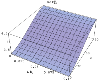
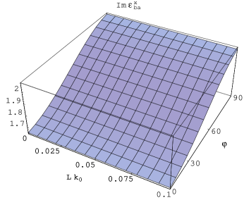
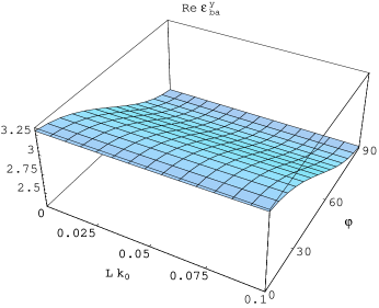
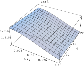
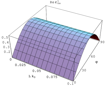
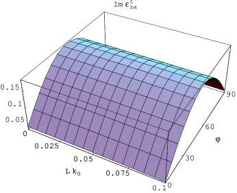
Figure 1: The real (left) and imaginary (right) parts of the components of $\underline{\underline{\hat{\epsilon}}}_{\,ba}(0,0,0)\equiv\underline{\underline{\epsilon}}_{\,ba}$ plotted against the relative correlation length $Lk_{\scriptscriptstyle 0}$ and orientation angle $\varphi$ (in degrees) of component phase $a$. The dissipation parameter $\delta=1$.

Consider the four relative permittivity scalars, $\epsilon^{x,y,z,t}_{ba}$, in the unrotated reference frame, i.e., $\underline{\underline{\hat{\epsilon}}}_{\,ba}(0,0,0)\equiv\underline{\underline{\epsilon}}_{\,ba}$. The $\epsilon^{x,y,z,t}_{ba}$ values calculated with the dissipation parameter $\delta=1$ are plotted in Figure 1, as functions of the orientation angle $\varphi$ of component phase $a$ and the relative correlation length $Lk_{\scriptscriptstyle 0}$. At $\varphi=0$ (and also at $\varphi=\pi$), the preferred axes of both component phases are aligned. Accordingly, the HCM is uniaxial with $\epsilon^{x}_{ba}=\epsilon^{y}_{ba}$. For $\varphi\neq 0$ (and also $\varphi\neq\pi$), the HCM is biaxial. As $\varphi\rightarrow\pi/2$, the HCM biaxial structure becomes orthorhombic since $\epsilon^{t}_{ba}\rightarrow 0$. For intermediate values of $\varphi\in(0,\pi/2)$, the HCM has the general non–orthorhombic biaxial form [18]. The correlation length is found to have only a marginal influence on $\epsilon^{x,y,z,t}_{ba}$ for $\delta=1$.

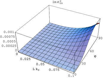
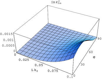
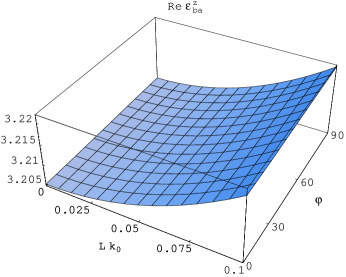
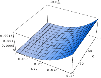
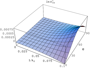
Figure 2: As Figure 1 but with $\delta=0$.

The HCM constitutive parameters corresponding to those of Figure 1, but arising from nondissipative component phases (i.e., $\delta=0$), are presented in Figure 2. The absence of dissipation in the component phases has little effect on the real parts of $\epsilon^{x,y,z,t}_{ba}$. However, the imaginary parts of $\epsilon^{x,y,z,t}_{ba}$ are much altered. Since the component phases are nondissipative, the imaginary parts of $\epsilon^{x,y,z,t}_{ba}$ are null–valued at zero correlation length. As the correlation length increases, the loss due to the effects of coherent scattering becomes greater. Hence, the magnitudes of the imaginary parts of $\epsilon^{x,y,z,t}_{ba}$ are observed to increase in Figure 2 as $Lk_{\scriptscriptstyle 0}$ grows. Furthermore, it is clear from Figure 2 that the rate of increase of these imaginary parts is sensitively dependent upon the orientation angle $\varphi$ of the component phase $a$.

4.2 Zeros of $Y$

The condition $Y=0$ can be satisfied at two distinct HCM orientations. These orientations are denoted by the angular coordinates $(\alpha_{1},\beta_{1})$ and $(\alpha_{2},\beta_{2})$. With the normalized correlation length fixed at $Lk_{\scriptscriptstyle 0}=0.1$, the $(\alpha_{1},\beta_{1})$ and $(\alpha_{2},\beta_{2})$ angular coordinates are graphed as functions of $\varphi$ in Figure 3 for the dissipation parameter values $\delta=0.0,0.1,0.5$ and $1$. In particular, observe that the two distinct solutions of $Y(\alpha,\beta,0)=0$ exist even when the component material phases are nondissipative (i.e., $\delta=0$). The angular coordinates $(\alpha_{1},\beta_{1})$ and $(\alpha_{2},\beta_{2})$ are clearly sensitive to both $\varphi$ and $\delta$.

Values of $|W|$, corresponding to the angular coordinates $(\alpha_{1},\beta_{1})$ and $(\alpha_{2},\beta_{2})$ of Figure 3, are plotted against $\varphi$ in Figure 4. For $\varphi>0$, the magnitude $|W|>0$. In particular, the inequality $|W|>0$ holds for $\delta=0$ (which is not clearly illustrated in Figure 4 due to limited resolution). Therefore, Voigt waves can propagate along two distinct singular axes in the biaxial HCM, as specified by the angular coordinates $(\alpha_{1},\beta_{1})$ and $(\alpha_{2},\beta_{2})$, even when the HCM arises from nondissipative component phases. This conclusion stems solely from the incorporation of the correlation length in the SPFT, because the Maxwell Garnett and the Bruggeman formalisms would not predict Voigt wave propagation when both component phases are nondissipative [2].

The two orientations that zero the value of $Y$, as specified by the angular coordinates $(\alpha_{1},\beta_{1})$ and $(\alpha_{2},\beta_{2})$, are plotted against $\varphi$ in Figure 5 for the normalized correlation lengths $Lk_{\scriptscriptstyle 0}=0,0.05$ and $0.1$. The dissipation parameter is fixed at $\delta=1$. As in Figure 3, the two distinct directions described by $(\alpha_{1},\beta_{1})$ and $(\alpha_{2},\beta_{2})$ are sensitively dependent upon the orientation angle $\varphi$ of the component phase $a$. Furthermore, the two distinct directions persist in the limit $Lk_{\scriptscriptstyle 0}\rightarrow 0$. The influence of $Lk_{\scriptscriptstyle 0}$ upon the angular coordinates $(\alpha_{1},\beta_{1})$ and $(\alpha_{2},\beta_{2})$ (as illustrated in Figure 5) is relatively minor in comparison with the influence of the dissipation parameter $\delta$ (as illustrated in Figure 3).

For the angular coordinates $(\alpha_{1},\beta_{1})$ and $(\alpha_{2},\beta_{2})$ of Figure 5, the corresponding values of $|W|$ are presented in Figure 6 as functions of $\varphi$. Clearly, $|W|>0$ for $\varphi>0$ when $Lk_{\scriptscriptstyle 0}=0,0.05$ and $0.1$. The magnitude of $Lk_{\scriptscriptstyle 0}$ has only a minor influence on $|W|$. Hence, the orientations of the singular axes, along which Voigt waves may propagate in the biaxial HCM, are modulated only to a minor degree by the correlation length.

5 Conclusions

The role of the correlation length in facilitating the propagation of Voigt waves in HCMs is delineated. Thereby, the importance of taking higher–order distributional statistics in homogenization studies into account is further emphasized. Specifically, we have demonstrated that

1. Voigt waves can propagate in HCMs arising from nondissipative component phases, provided that a nonzero correlation length is accommodated, according to the SPFT.

2. The orientations of singular axes in HCMs are sensitively dependent upon (i) the degree of dissipation exhibited by the component phases and the (ii) the orientation of the preferred axes of the component material phases. By comparison, the correlation length plays only a secondary role in determining the singular axis orientations.

Acknowledgement: TGM acknowledges the financial support of The Nuffield Foundation.

Appendix

We establish here a surface integral representation of $\underline{\underline{P}}$ (12), amenable to numerical evaluation. A straightforward specialization of the evaluation of $\underline{\underline{P}}$ for bianisotropic HCMs [12] yields the volume integral

$$\underline{\underline{P}}=\frac{f_{a}f_{b}}{2\pi^{2}\,i\omega}\int d^{3}{\bf q}\;\;\frac{(q/\omega)^{2}\,\underline{\underline{\alpha}}+\underline{\underline{\beta}}}{(q/\omega)^{4}\,t_{C}+(q/\omega)^{2}\,t_{B}+t_{A}}\,\left(\,\frac{\sin qL}{q}-L\cos qL\,\right)\,,$$ (19)

where the scalar quantities $t_{A},t_{B}$ and $t_{C}$ are given as

$$t_{A} = \mu_{\scriptscriptstyle 0}^{3}\epsilon^{z}_{Br}\left[\,\epsilon^{x}_{Br}\epsilon^{y}_{Br}-\left(\epsilon^{t}_{Br}\right)^{2}\right],$$ (20)

$$t_{B} = -\mu_{\scriptscriptstyle 0}^{2}\left\{\,\epsilon^{z}_{Br}\left(\epsilon^{x}_{Br}+\epsilon^{y}_{Br}\right)\cos^{2}\theta+\left[\Gamma^{\phi}_{Br}\epsilon^{z}_{Br}+\epsilon^{x}_{Br}\epsilon^{y}_{Br}-\left(\epsilon^{t}_{Br}\right)^{2}\right]\sin^{2}\theta\right\},$$ (21)

$$t_{C} = \mu_{\scriptscriptstyle 0}\left(\epsilon^{z}_{Br}\cos^{2}\theta+\Gamma^{\phi}_{Br}\sin^{2}\theta\right).$$ (22)

The dyadic quantities $\underline{\underline{\alpha}}$ and $\underline{\underline{\beta}}$ are specified as

$$\underline{\underline{\alpha}} = \underline{\underline{T}}_{\,B}-\frac{t_{B}}{t_{C}}\,\underline{\underline{T}}_{\,C},$$ (23)

$$\underline{\underline{\beta}} = \underline{\underline{T}}_{\,A}-\frac{t_{A}}{t_{C}}\,\underline{\underline{T}}_{\,C},$$ (24)

with

$$\underline{\underline{T}}_{\,A} = \mu_{\scriptscriptstyle 0}^{3}\,\mbox{adj}\left(\underline{\underline{\epsilon}}_{Br}\right),$$ (25)

$$\underline{\underline{T}}_{\,B} = -\mu_{\scriptscriptstyle 0}^{2}\Big{\{}\,\left[\epsilon^{z}_{Br}+\left(\epsilon^{y}_{Br}-\epsilon^{z}_{Br}\sin^{2}\phi\right)\sin^{2}\theta\right]\,\hat{{\bf x}}\,\hat{{\bf x}}$$ (26)

$$+\left[\epsilon^{z}_{Br}+\left(\epsilon^{x}_{Br}-\epsilon^{z}_{Br}\cos^{2}\phi\right)\sin^{2}\theta\right]\,\hat{{\bf y}}\,\hat{{\bf y}}$$

$$+\left[\left(\epsilon^{x}_{Br}+\epsilon^{y}_{Br}\right)\cos^{2}\theta+\Gamma^{\phi}_{Br}\sin^{2}\theta\right]\,\hat{{\bf z}}\,\hat{{\bf z}}$$

$$+\left[\left(\epsilon^{z}_{Br}\sin\phi\cos\phi-\epsilon^{t}_{Br}\right)\sin^{2}\theta\right]\,\left(\hat{{\bf x}}\,\hat{{\bf y}}+\hat{{\bf y}}\,\hat{{\bf x}}\right)\,\Big{\}},$$

$$\underline{\underline{T}}_{\,C} = \mu_{\scriptscriptstyle 0}\Big{[}\sin^{2}\theta\cos^{2}\phi\,\hat{{\bf x}}\,\hat{{\bf x}}+\sin^{2}\theta\sin^{2}\phi\,\hat{{\bf y}}\,\hat{{\bf y}}$$ (27)

$$+\cos^{2}\theta\,\hat{{\bf z}}\,\hat{{\bf z}}+\sin^{2}\theta\cos\phi\sin\phi\,\left(\hat{{\bf x}}\,\hat{{\bf y}}+\hat{{\bf y}}\,\hat{{\bf x}}\right)\Big{]}.$$

Let

$$\rho_{\pm}=\omega^{2}\,\frac{-t_{B}\pm\sqrt{t^{2}_{B}-4t_{A}t_{C}}}{2\,t_{C}}.$$ (28)

In the long–wavelength regime, i.e., $|\,L\sqrt{\rho_{\pm}}\,|\ll 1$ [12], the application of residue calculus to (19) delivers the surface integral

$$\underline{\underline{P}} = \frac{L^{2}f_{a}f_{b}\,\omega}{4\pi i}\int^{2\pi}_{0}d\phi\int^{\pi}_{0}d\theta\;\;\frac{\sin\theta}{3\,\sqrt{t^{2}_{B}-4t_{A}t_{C}}}\times$$ (29)

$$\Bigg{\{}\,\frac{1}{\omega^{2}}\left[\,\frac{3}{2}\,\left(\,\rho_{+}-\rho_{-}\,\right)+iL\left(\,\rho_{+}\sqrt{\rho_{+}}-\rho_{-}\sqrt{\rho_{-}}\,\right)\right]\underline{\underline{\alpha}}+iL\,\left(\,\sqrt{\rho_{+}}-\sqrt{\rho_{-}}\,\right)\underline{\underline{\beta}}\,\Bigg{\}}.$$

Standard numerical techniques may be straightforwardly applied to evaluate (29).

Figure 3: The $\alpha$ and $\beta$ angular coordinates (in degrees) of the zeros of $Y(\alpha,\beta,0)$ plotted against the orientation angle $\varphi$ (in degrees) of component phase $a$. The relative correlation length $Lk_{\scriptscriptstyle 0}=0.1$.

Figure 4: The values of $|W(\alpha_{1,2},\beta_{1,2},0)|$ corresponding to the $(\alpha_{1},\beta_{1})$ and $(\alpha_{2},\beta_{2})$ angular coordinates of Figure 3, as functions of the orientation angle $\varphi$ (in degrees) of the component phase $a$.

Figure 5: As Figure 3 but with dissipation parameter $\delta=1$ and relative correlation length $Lk_{\scriptscriptstyle 0}=0,0.05$ and $0.1$.

Figure 6: The values of $|W(\alpha_{1,2},\beta_{1,2},0)|$ corresponding to the $(\alpha_{1},\beta_{1})$ and $(\alpha_{2},\beta_{2})$ angular coordinates of Figure 5, as functions of the orientation angle $\varphi$ (in degrees) of the component phase $a$.

References

• [1] Walser R M 2003 Metamaterials Introduction to Complex Mediums for Optics and Electromagnetics ed WS Weiglhofer and A Lakhtakia (Bellingham, WA, USA: SPIE Optical Engineering Press) (in press)
• [2] Mackay TG and Lakhtakia A 2003 Voigt wave propagation in biaxial composite materials J. Opt. A: Pure Appl. Opt. 5 91–95
• [3] Voigt W 1902 On the behaviour of pleochroitic crystals along directions in the neighbourhood of an optic axis Phil. Mag. 4 90–97
• [4] Lakhtakia A 1998 Anomalous axial propagation in helicoidal bianisotropic media Opt. Commun. 157 193–201
• [5] Berry MV and Dennis MR 2003 The optical singularities of birefringent dichroic chiral crystals Proc. R. Soc. Lond. A 459 1261–1292
• [6] Singh O N and Lakhtakia A (ed) 2000 Electromagnetic Fields in Unconventional Materials and Structures (New York: Wiley)
• [7] Gerardin J and Lakhtakia A 2001 Conditions for Voigt wave propagation in linear, homogeneous, dielectric mediums Optik 112 493–495
• [8] Khapalyuk A P 1962 On the theory of circular optical axes Opt. Spectrosc. (USSR) 12 52–54
• [9] Lakhtakia A (ed) 1996 Selected Papers on Linear Optical Composite Materials (Bellingham, WA, USA: SPIE Optical Engineering Press)
• [10] Tsang L and Kong J A 1981 Scattering of electromagnetic waves from random media with strong permittivity fluctuations Radio Sci. 16 303–320
• [11] Genchev ZD 1992 Anisotropic and gyrotropic version of Polder and van Santen’s mixing formula Waves Random Media 2 99–110
• [12] Mackay T G, Lakhtakia A and Weiglhofer W S 2000 Strong–property–fluctuation theory for homogenization of bianisotropic composites: formulation Phys. Rev. E 62 6052–6064 Erratum 2001 63 049901(E)
• [13] Tsang L, Kong J A and Newton R W 1982 Application of strong fluctuation random medium theory to scattering of electromagnetic waves from a half–space of dielectric mixture IEEE Trans. Antennas Propagat. 30 292–302
• [14] Mackay T G, Lakhtakia A and Weiglhofer W S 2001 Homogenisation of similarly oriented, metallic, ellipsoidal inclusions using the bilocally approximated strong–property–fluctuation theory Opt. Commun. 197 89–95
• [15] Michel B 1997 A Fourier space approach to the pointwise singularity of an anisotropic dielectric medium Int. J. Appl. Electromagn. Mech. 8 219–227
• [16] Frisch U 1970 Wave propagation in random media Probabilistic Methods in Applied Mathematics Vol. 1 ed A T Bharucha–Reid (London: Academic Press) pp75–198
• [17] Arfken G B and Weber H J 1995 Mathematical Methods for Physicists 4th Edition (London: Academic Press)
• [18] Mackay T G and Weiglhofer W S 2000 Homogenization of biaxial composite materials: dissipative anisotropic properties J. Opt. A: Pure Appl. Opt. 2 426–432
Refer to caption
Refer to caption
Refer to caption
Refer to caption
Refer to caption
Refer to caption
Refer to caption
Refer to caption