We consider an anisotropic homogenized composite medium (HCM) arising from isotropic particulate component phases based on ellipsoidal geometries. For cubically nonlinear component phases, the corresponding zeroth-order strong-permittivity-fluctuation theory (SPFT) (which is equivalent to the Bruggeman homogenization formalism) and second-order SPFT are established and used to estimate the constitutive properties of the HCM. The relationship between the component phase particulate geometry and the HCM constitutive properties is explored. Significant differences are highlighted between the estimates of the Bruggeman homogenization formalism and the second-order SPFT estimates. The prospects for nonlinearity enhancement are investigated.

1 Introduction

The constitutive properties of a homogenized composite medium (HCM) are determined by both the constitutive properties and the topological properties of its component phases [1]–[5]. In particular, component phases based on nonspherical particulate geometries may give rise to anisotropic HCMs, despite the component phases themselves being isotropic with respect to their electromagnetic properties. Such geometrically-derived anisotropy has been extensively characterized for linear dielectric HCMs [6]–[8] and more general bianisotropic HCMs [8]–[10]. For weakly nonlinear HCMs, the role of the component phase particulate geometry was emphasized recently in this journal by Goncharenko, Popelnukh and Venger [11], using an approach founded on the mean-field approximation. However, their analysis was restricted to the Maxwell Garnett homogenization formalism [3, 12]. A more comprehensive study is communicated here based on the strong-permittivity-fluctuation theory (SPFT) [13]. In contrast to the aforementioned Maxwell Garnett approach [11], the SPFT approach (i) incorporates higher-order statistics to describe the component phase distributions; (ii) is not restricted to only dilute composites; and (iii) is not restricted to only weakly nonspherical particulate geometries.

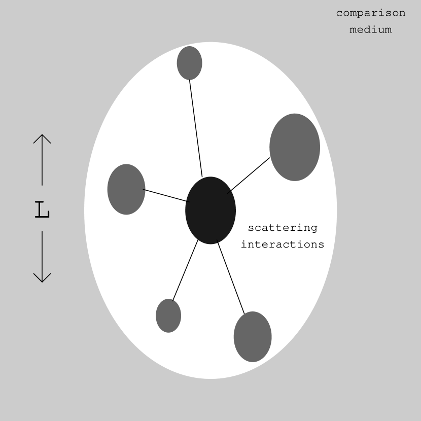
Figure 1: Schematic diagram illustrating the bilocally-approximated SPFT for ellipsoidal component phase geometry: pair-wise scattering interactions are accommodated between ellipsoidal scattering centres contained within an ellipsoidal correlation region of linear dimensions $L$.

The early development of the SPFT concerned wave propagation in continuous random mediums [14, 15], but more recently the theory has been applied to the estimation of HCM constitutive parameters [16, 17]. The SPFT represents a significant advance over conventional homogenization formalisms, such as the Maxwell Garnett approach and the Bruggeman approach [3, 6], through incorporating a comprehensive description of the distributional statistics of the HCM component phases. In estimating the constitutive parameters of an HCM, the SPFT employs a Feynman–diagrammatic technique to calculate iterative refinements to the constitutive parameters of a comparison medium; successive iterates incorporate successively higher–order spatial correlation functions. It transpires that the SPFT comparison medium is equivalent to the effective medium of the (symmetric) Bruggeman homogenization theory [20, 21]. In principle, correlation functions of arbitrarily high order can be accommodated in the SPFT. However, the theory is most widely-implemented at the level of the bilocal approximation (i.e., second-order approximation), wherein a two-point covariance function and its associated correlation length $L$ characterize the component phase distributions. As indicated in figure 1, coherent interactions between pairs of scattering centres within a region of linear dimensions $L$ are incorporated in the bilocal SPFT; scattering centres separated by distances much greater than $L$ are assumed to act independently. Thereby, the SPFT provides an estimation of coherent scattering losses, unlike the Maxwell Garnett and Bruggeman homogenization formalisms. Notice that the bilocally–approximated SPFT gives rise to the Bruggeman homogenization formalism in the limit $L\rightarrow 0$ [21].

The SPFT has been widely applied to linear homogenization scenarios, where generalizations have been developed for anisotropic dielectric [18, 19], isotropic chiral [20] and bianisotropic [21, 22] HCMs. Investigations of the trilocally-approximated SPFT for isotropic HCMs have recently confirmed the convergence of the second-order theory [17, 23, 24]. In the weakly nonlinear regime, developments of the bilocally-approximated SPFT have been restricted to isotropic HCMs, based on spherical component phase geometry [16, 17, 24]. The present study advances the nonlinear SPFT through developing the theory for cubically nonlinear, anisotropic HCMs. Furthermore, it is assumed that the component phases are composed of electrically-small ellipsoidal particles. The relationship between the HCM constitutive parameters and the underlying particulate geometry of the component phases is investigated via a representative numerical example.

In our notational convention, dyadics are double underlined whereas vectors are in bold face. The inverse, adjoint, determinant and trace of a dyadic $\underline{\underline{A}}$ are denoted by $\underline{\underline{A}}^{-1}$, $\underline{\underline{A}}^{adj}$ , $\mbox{det}\,\left[\,\underline{\underline{A}}\,\right]$ and $\mbox{tr}\,\left[\,\underline{\underline{A}}\,\right]$, respectively. The identity dyadic is represented by $\,\underline{\underline{I}}\,$. The ensemble average of a quantity $\psi$ is written as $\langle\,\psi\,\rangle$. The permittivity and permeability of free space (i.e., vacuum) are given by $\epsilon_{\scriptscriptstyle 0}$ and $\mu_{\scriptscriptstyle 0}$, respectively; $k_{\scriptscriptstyle 0}=\omega\sqrt{\epsilon_{\scriptscriptstyle 0}\mu_{\scriptscriptstyle 0}}$ is the free-space wavenumber while $\omega$ is the angular frequency.

2 Homogenization generalities

2.1 Component phases

Consider the homogenization of a two-phase composite with component phases labelled as $a$ and $b$. The component phases are taken to be isotropic dielectric mediums with permittivities

$$\epsilon_{\ell}=\epsilon_{\ell\,0}+\chi_{\ell}\,|\,{\bf E}_{\,\ell}\,|^{2},\hskip 85.35826pt(\ell=a,b),$$ (1)

where $\epsilon_{\ell\,0}$ is the linear permittivity, $\chi_{\ell}$ is the nonlinear susceptibility, and $|\,{\bf E}_{\,\ell}\,|^{2}$ is the electric field developed inside a region of phase $\ell$ by illumination of the composite medium. We assume weak nonlinearity; i.e., $|\,\epsilon_{\ell\,0}\,|\gg|\,\chi_{\ell}\,|\,|\,{\bf E}_{\,\ell}\,|^{2}$. Notice that such electrostrictive mediums as characterized by (1) can induce Brillouin scattering which is often a strong process [25]. The component phases $a$ and $b$ are taken to be randomly distributed as identically-orientated, conformal ellipsoids. The shape dyadic

$$\underline{\underline{U}}=\frac{1}{\sqrt[3]{U_{x}U_{y}U_{z}}}\;\mbox{diag}(U_{x},U_{y},U_{z}),\hskip 71.13188pt(U_{x},U_{y},U_{z}>0),$$ (2)

parameterizes the conformal ellipsoidal surfaces as

$${\bf r}_{\,e}(\theta,\phi)=\eta\,\underline{\underline{U}}\mbox{ \tiny{${}^{\bullet}$} }{\bf\hat{r}}\,(\theta,\phi),$$ (3)

where ${\bf\hat{r}}\,(\theta,\phi)$ is the radial unit vector specified by the spherical polar coordinates $\theta$ and $\phi$. Thus, a wide range of ellipsoidal particulate shapes, including highly elongated forms, can be accommodated. The linear ellipsoidal dimensions, as determined by $\eta$, are assumed to be sufficiently small that the electromagnetic long-wavelength regime pertains.

In the SPFT, statistical moments of the characteristic functions

$$\Phi_{\ell}({\bf r})=\left\{\begin{array}[]{ll}1,&\qquad{\bf r}\in V_{\,\ell},\\ &\qquad\qquad\qquad\qquad\qquad\qquad(\ell=a,b),\\ 0,&\qquad{\bf r}\not\in V_{\,\ell},\end{array}\right.$$ (4)

are utilized to take account of the component phase distributions. The volume fraction of phase $\ell$, namely $f_{\ell}$ , is given by the first statistical moment of $\Phi_{\ell}$ ; i.e., $\langle\,\Phi_{\ell}({\bf r})\,\rangle=f_{\ell}$ . Clearly, $f_{a}+f_{b}=1$. The second statistical moment of $\Phi_{\ell}$ provides a two-point covariance function; we adopt the physically-motivated form [26]

$$\langle\,\Phi_{\ell}({\bf r})\,\Phi_{\ell}({\bf r}^{\prime})\,\rangle=f_{\ell}\,\left[1+\left(\,f_{\ell}-1\,\right)\,\mathcal{H}\left(\,\sigma-L\,\right)\,\right]\,,$$ (5)

where $\mathcal{H}$ is the Heaviside function (i.e., $\mathcal{H}(x)=\int^{x}_{-\infty}\delta(y)\,dy$ where $\delta$ is the Dirac delta function), $\sigma=|\,\underline{\underline{U}}^{-1}\mbox{ \tiny{${}^{\bullet}$} }{\bf R}\,|$ with ${\bf R}={\bf r}-{\bf r}^{\prime}$, and $L>0$ is the correlation length. The specific nature of the covariance function has been found to exert little influence on the SPFT estimates for linear [19] and weakly nonlinear [17] HCMs.

2.2 Homogenized composite medium

Let ${\bf E}_{\,HCM}$ denote the spatially-averaged electric field in the HCM. In this communication we derive the estimate

$$\underline{\underline{\epsilon}}_{\,ba} = \underline{\underline{\epsilon}}_{\,ba0}+\underline{\underline{\chi}}_{\,ba}\,|\,{\bf E}_{\,HCM}\,|^{2}$$ (6)

$$= \mbox{diag}\left(\epsilon^{x}_{ba0},\,\epsilon^{y}_{ba0},\,\epsilon^{z}_{ba0}\right)+\mbox{diag}\left(\chi^{x}_{ba},\,\chi^{y}_{ba},\,\chi^{z}_{ba}\right)\,|\,{\bf E}_{\,HCM}\,|^{2}$$ (7)

of the HCM permittivity. The bilocally-approximated SPFT is utilized (hence the subscripts ba in (6), (7) ). Note that the Bruggeman estimate of the HCM permittivity, namely

$$\underline{\underline{\epsilon}}_{\,Br} = \underline{\underline{\epsilon}}_{\,Br0}+\underline{\underline{\chi}}_{\,Br}\,|\,{\bf E}_{\,HCM}\,|^{2}$$ (8)

$$= \mbox{diag}\left(\epsilon^{x}_{Br0},\,\epsilon^{y}_{Br0},\,\epsilon^{z}_{Br0}\right)+\mbox{diag}\left(\chi^{x}_{Br},\,\chi^{y}_{Br},\,\chi^{z}_{Br}\right)\,|\,{\bf E}_{\,HCM}\,|^{2},$$ (9)

characterizes the comparison medium which is adopted in the bilocally-approximated SPFT [21]. As the Bruggeman homogenization formalism — in which the component phases $a$ and $b$ are treated symmetrically [6] — provides the comparison medium, the SPFT homogenization approach (like the Bruggeman formalism) is applicable for all volume fractions $f_{a}\in(0,1)$.

2.3 Depolarization and polarizability dyadics

The depolarization dyadic $\underline{\underline{D}}$ is a key element in both Bruggeman and SPFT homogenizations. It provides the electromagnetic response of a $\underline{\underline{U}}$-shaped exclusion volume, immersed in a homogeneous background, in the limit $\eta\rightarrow 0$. For the component phases described by (1) and (2), we find [27, 28]

$$\underline{\underline{D}} = \frac{1}{i\,\omega\,4\pi}\,\int^{2\pi}_{0}\;d\phi\,\int^{\pi}_{0}\;d\theta\;\sin\theta\,\left(\,\frac{1}{\mbox{tr}\left[\,\underline{\underline{\epsilon}}_{\,Br}\mbox{ \tiny{${}^{\bullet}$} }\underline{\underline{A}}\,\right]}\,\underline{\underline{A}}\,\right)\,,$$ (10)

wherein

$$\underline{\underline{A}}=\mbox{diag}\,\left(\,\frac{\sin^{2}\theta\,\cos^{2}\phi}{U^{2}_{x}},\,\frac{\sin^{2}\theta\,\sin^{2}\phi}{U^{2}_{y}},\,\frac{\cos^{2}\theta}{U^{2}_{z}}\,\right)\,.$$ (11)

The integrations of (10) reduce to elliptic function representations [29]. In the case of spheroidal particulate geometries, hyperbolic functions provide an evaluation of $\underline{\underline{D}}$ [27], while for the degenerate isotropic case $U_{x}=U_{y}=U_{z}$ we have the well-known result $\underline{\underline{D}}=\left(1/i\omega 3\right)\underline{\underline{\epsilon}}^{-1}_{\,Br}$ [30]. We express $\underline{\underline{D}}$ as the sum of linear and weakly nonlinear parts

$$\underline{\underline{D}}=\underline{\underline{D}}_{\,0}+\underline{\underline{D}}_{\,1}\,|\,{\bf E}_{\,HCM}\,|^{2},$$ (12)

with

$$\underline{\underline{D}}_{\,0}=\frac{1}{i\,\omega\,4\pi}\,\int^{2\pi}_{0}\;d\phi\,\int^{\pi}_{0}\;d\theta\;\sin\theta\,\left(\,\frac{1}{\mbox{tr}\left[\,\underline{\underline{\epsilon}}_{\,Br0}\mbox{ \tiny{${}^{\bullet}$} }\underline{\underline{A}}\,\right]}\,\underline{\underline{A}}\,\right)\,,$$ (13)

$$\underline{\underline{D}}_{\,1}=-\frac{1}{i\,\omega\,4\pi}\,\int^{2\pi}_{0}\;d\phi\,\int^{\pi}_{0}\;d\theta\;\sin\theta\,\left[\,\frac{\mbox{tr}\left[\,\underline{\underline{\chi}}_{\,Br}\mbox{ \tiny{${}^{\bullet}$} }\underline{\underline{A}}\,\right]}{\left(\,\mbox{tr}\left[\,\underline{\underline{\epsilon}}_{\,Br0}\mbox{ \tiny{${}^{\bullet}$} }\underline{\underline{A}}\,\right]\,\right)^{2}}\,\underline{\underline{A}}\,\right]\,.$$ (14)

A convenient construction in homogenization formalisms is the polarizability dyadic $\underline{\underline{X}}_{\,\ell}$, defined as

$$\underline{\underline{X}}_{\,\ell}=-i\,\omega\,\left(\,\epsilon_{\ell}\,\underline{\underline{I}}-\underline{\underline{\epsilon}}_{\,Br}\,\right)\mbox{ \tiny{${}^{\bullet}$} }\underline{\underline{\Gamma}}^{-1}_{\,\ell}\,,\hskip 85.35826pt(\ell=a,b),$$ (15)

where

$$\underline{\underline{\Gamma}}_{\,\ell}=\left[\,\underline{\underline{I}}+i\omega\,\underline{\underline{D}}\mbox{ \tiny{${}^{\bullet}$} }\left(\,\epsilon_{\ell}\,\underline{\underline{I}}-\underline{\underline{\epsilon}}_{\,Br}\,\right)\,\right]\,.$$ (16)

Let us proceed to calculate the linear and nonlinear contributions in the decomposition

$$\underline{\underline{X}}_{\,\ell} = \underline{\underline{X}}_{\,\ell\,0}+\underline{\underline{X}}_{\,\ell\,1}\,|\,{\bf E}_{\,HCM}\,|^{2}\,,\hskip 85.35826pt(\ell=a,b).$$ (17)

Under the assumption of weak nonlinearity, we express (16) in the form

$$\underline{\underline{\Gamma}}_{\,\ell} = \underline{\underline{\Gamma}}_{\,\ell\,0}+\underline{\underline{\Gamma}}_{\,\ell\,1}\,|\,{\bf E}_{\,HCM}\,|^{2}\,,$$ (18)

with linear term

$$\underline{\underline{\Gamma}}_{\,\ell\,0}=\mbox{diag}\left(\Gamma^{x}_{\ell\,0},\,\Gamma^{y}_{\ell\,0},\,\Gamma^{z}_{\ell\,0}\right)=\underline{\underline{I}}+i\omega\,\underline{\underline{D}}_{\,0}\mbox{ \tiny{${}^{\bullet}$} }\left(\,\epsilon_{\ell\,0}\,\underline{\underline{I}}-\underline{\underline{\epsilon}}_{\,Br0}\,\right)\,,$$ (19)

and nonlinear term

$$\underline{\underline{\Gamma}}_{\,\ell\,1}=\mbox{diag}\left(\Gamma^{x}_{\ell\,1},\,\Gamma^{y}_{\ell\,1},\,\Gamma^{z}_{\ell\,1}\right)=i\omega\,\left[\,\underline{\underline{D}}_{\,0}\mbox{ \tiny{${}^{\bullet}$} }\left(\,g_{\ell}\,\chi_{\ell}\,\underline{\underline{I}}-\underline{\underline{\chi}}_{\,Br}\,\right)+\underline{\underline{D}}_{\,1}\mbox{ \tiny{${}^{\bullet}$} }\left(\,\epsilon_{\ell\,0}\,\underline{\underline{I}}-\underline{\underline{\epsilon}}_{\,Br0}\,\right)\,\right]\,.$$ (20)

The local field factor

$$g_{\ell}=\frac{d\,|\,{\bf E}_{\ell}\,|^{2}}{d\,|\,{\bf E}_{\,HCM}\,|^{2}}\,,\hskip 85.35826pt(\ell=a,b),$$ (21)

has been incorporated in deriving (18)–(20), via the Maclaurin series expansion $\epsilon_{\ell}=\epsilon_{\ell\,0}+g_{\ell}\,\chi_{\ell}\,|\,{\bf E}_{\,HCM}\,|^{2}$. An appropriate estimation of the local field factor is provided by [31]

$$g_{\ell}=\left|\,\frac{1}{3}\,\left(\,\mbox{tr}\left[\,\underline{\underline{\Gamma}}^{-1}_{\,\ell\,0}\,\right]\,\right)\,\right|^{2}.$$ (22)

Thus, the inverse of $\underline{\underline{\Gamma}}_{\,\ell}$ is given as

$$\underline{\underline{\Gamma}}^{-1}_{\,\ell} = \underline{\underline{\Gamma}}^{-1}_{\,\ell\,0}+\underline{\underline{\Lambda}}_{\,\ell}\,|\,{\bf E}_{\,HCM}\,|^{2}\,,$$ (23)

wherein

$$\underline{\underline{\Lambda}}_{\,\ell}=\frac{1}{\det\left[\,\underline{\underline{\Gamma}}_{\,\ell\,0}\,\right]}\left[\,\mbox{diag}\,\Big{(}\,\Gamma^{y}_{\ell\,1}\Gamma^{z}_{\ell\,0}+\Gamma^{y}_{\ell\,0}\Gamma^{z}_{\ell\,1},\,\Gamma^{z}_{\ell\,1}\Gamma^{x}_{\ell\,0}+\Gamma^{z}_{\ell\,0}\Gamma^{x}_{\ell\,1},\,\Gamma^{y}_{\ell\,1}\Gamma^{x}_{\ell\,0}+\Gamma^{y}_{\ell\,0}\Gamma^{x}_{\ell\,1}\,\Big{)}-\rho_{\ell}\,\underline{\underline{\Gamma}}^{-1}_{\,\ell\,0}\,\right],$$

(24)

and

$$\rho_{\ell}=\Gamma^{x}_{\ell\,0}\Gamma^{y}_{\ell\,0}\Gamma^{z}_{\ell\,1}+\Gamma^{x}_{\ell\,0}\Gamma^{y}_{\ell\,1}\Gamma^{z}_{\ell\,0}+\Gamma^{x}_{\ell\,1}\Gamma^{y}_{\ell\,0}\Gamma^{z}_{\ell\,0}\,.$$ (25)

Combining (23) and (24) with (15), and separating linear and nonlinear terms, provides

$$\left.\begin{array}[]{l}\underline{\underline{X}}_{\,\ell\,0}=-i\,\omega\,\left(\,\epsilon_{\ell\,0}\,\underline{\underline{I}}-\underline{\underline{\epsilon}}_{\,Br0}\,\right)\mbox{ \tiny{${}^{\bullet}$} }\underline{\underline{\Gamma}}^{-1}_{\,\ell\,0}\\ \underline{\underline{X}}_{\,\ell\,1}=-i\,\omega\,\left[\,\left(\,g_{\ell}\,\chi_{\ell}\,\underline{\underline{I}}-\underline{\underline{\chi}}_{\,Br}\,\right)\mbox{ \tiny{${}^{\bullet}$} }\underline{\underline{\Gamma}}^{-1}_{\,\ell\,0}\,+\left(\,\epsilon_{\ell\,0}\,\underline{\underline{I}}-\underline{\underline{\epsilon}}_{\,Br0}\,\right)\mbox{ \tiny{${}^{\bullet}$} }\underline{\underline{\Lambda}}_{\,\ell}\,\right]\end{array}\right\},\hskip 42.67912pt(\ell=a,b).$$ (26)

2.4 Bruggeman homogenization

The Bruggeman estimates of the HCM linear permittivity $\underline{\underline{\epsilon}}_{\,Br0}$ and nonlinear susceptibility $\underline{\underline{\chi}}_{\,Br}$ are delivered through solving the nonlinear equations [3, 6, 31]

$$f_{a}\,\underline{\underline{X}}_{\,a\mbox{j}}+f_{b}\,\underline{\underline{X}}_{\,b\mbox{j}}=\underline{\underline{0}}\,,\hskip 85.35826pt(\,\mbox{j}=0,1).$$ (27)

Recursive procedures for this purpose provide the $p^{\mbox{th}}$ iterates [4, 24]

$$\left.\begin{array}[]{l}\underline{\underline{\epsilon}}_{\,ba0}\,[p]=\mathcal{T}_{\epsilon}\,\left\{\,\underline{\underline{\epsilon}}_{\,ba0}\,[p-1]\,\right\}\\ \underline{\underline{\chi}}_{\,ba}\,[p]=\mathcal{T}_{\chi}\,\left\{\,\underline{\underline{\chi}}_{\,ba}\,[p-1]\,\right\}\end{array}\right\}$$ (28)

in terms of the $(p-1)^{\mbox{th}}$ iterates, wherein the operators $\mathcal{T}_{\epsilon,\chi}$ are defined by

$$\mathcal{T}_{\epsilon}\,\left\{\,\underline{\underline{\epsilon}}_{\,ba0}\,\right\} = \left(\,f_{a}\,\epsilon_{a0}\,\underline{\underline{\Gamma}}^{-1}_{\,a0}+f_{b}\,\epsilon_{b0}\,\underline{\underline{\Gamma}}^{-1}_{\,b0}\,\right)\mbox{ \tiny{${}^{\bullet}$} }\left(\,f_{a}\,\underline{\underline{\Gamma}}^{-1}_{\,a0}+f_{b}\,\underline{\underline{\Gamma}}^{-1}_{\,b0}\,\right)^{-1}\,,$$

$$\mathcal{T}_{\chi}\,\left\{\,\underline{\underline{\chi}}_{\,ba}\,\right\} = \left\{f_{a}\left[g_{a}\,\chi_{a}\,\underline{\underline{\Gamma}}^{-1}_{\,a0}+\left(\epsilon_{a0}\,\underline{\underline{I}}-\underline{\underline{\epsilon}}_{\,ba0}\right)\mbox{ \tiny{${}^{\bullet}$} }\underline{\underline{\Lambda}}_{\,a}\right]+f_{b}\left[g_{b}\,\chi_{b}\,\underline{\underline{\Gamma}}^{-1}_{\,b0}+\left(\epsilon_{b0}\,\underline{\underline{I}}-\underline{\underline{\epsilon}}_{\,ba0}\right)\mbox{ \tiny{${}^{\bullet}$} }\underline{\underline{\Lambda}}_{\,b}\right]\right\}$$ (29)

$$\mbox{ \tiny{${}^{\bullet}$} }\left(f_{a}\,\underline{\underline{\Gamma}}^{-1}_{\,a0}+f_{b}\,\underline{\underline{\Gamma}}^{-1}_{\,b0}\right)^{-1}\,,$$

while suitable initial values are given by

$$\left.\begin{array}[]{l}\underline{\underline{\epsilon}}_{\,ba0}\,[0]=\left(\,f_{a}\,\epsilon_{a0}+f_{b}\,\epsilon_{b0}\,\right)\,\underline{\underline{I}}\\ \underline{\underline{\chi}}_{\,ba}\,[0]=\left(\,f_{a}\,\chi_{a}+f_{b}\,\chi_{b}\,\right)\,\underline{\underline{I}}\end{array}\right\}\,.$$ (30)

3 The bilocally-approximated SPFT

The bilocally-approximated SPFT estimate of the HCM permittivity dyadic, as derived elsewhere [21], is given by

$$\underline{\underline{\epsilon}}_{\,ba}=\underline{\underline{\epsilon}}_{\,Br}-\frac{1}{i\,\omega}\,\left(\,\underline{\underline{I}}+\underline{\underline{\Sigma}}_{\,ba}\mbox{ \tiny{${}^{\bullet}$} }\underline{\underline{D}}\,\right)^{-1}\mbox{ \tiny{${}^{\bullet}$} }\underline{\underline{\Sigma}}_{\,ba}\,;$$ (31)

the mass operator term

$$\underline{\underline{\Sigma}}_{\,ba}=\left(\,\underline{\underline{X}}_{\,a}-\underline{\underline{X}}_{\,b}\,\right)\mbox{ \tiny{${}^{\bullet}$} }\underline{\underline{W}}\mbox{ \tiny{${}^{\bullet}$} }\left(\,\underline{\underline{X}}_{\,a}-\underline{\underline{X}}_{\,b}\,\right)$$ (32)

is specified in terms of the principal value integral

$$\underline{\underline{W}}=\mathcal{P}\,\int_{\sigma\leq L}\;d^{3}{\bf R}\>\;\underline{\underline{G}}_{\,Br}({\bf R}),$$ (33)

with $\underline{\underline{G}}_{\,Br}({\bf R})$ being the unbounded dyadic Green function of the comparison medium. Here we develop expressions for the linear and nonlinear contributions of $\underline{\underline{\epsilon}}_{\,ba}$, appropriate to the component phases specified in §2.

Under the assumption of weak nonlinearity, we express $\underline{\underline{W}}=\underline{\underline{W}}_{\,0}+\underline{\underline{W}}_{\,1}\,|\,{\bf E}_{\,HCM}\,|^{2}$; integral expressions for $\underline{\underline{W}}_{\,0}$ and $\underline{\underline{W}}_{\,1}$ are provided in the Appendix. Thereby, the linear and nonlinear terms in the mass operator decomposition $\underline{\underline{\Sigma}}_{\,ba}=\underline{\underline{\Sigma}}_{\,ba0}+\underline{\underline{\Sigma}}_{\,ba1}\,|\,{\bf E}_{\,HCM}\,|^{2}$ are given as

$$\underline{\underline{\Sigma}}_{\,ba0}=\left(\,\underline{\underline{X}}_{\,a0}-\underline{\underline{X}}_{\,b0}\,\right)\mbox{ \tiny{${}^{\bullet}$} }\underline{\underline{W}}_{\,0}\mbox{ \tiny{${}^{\bullet}$} }\left(\,\underline{\underline{X}}_{\,a0}-\underline{\underline{X}}_{\,b0}\,\right),$$ (34)

$$\underline{\underline{\Sigma}}_{\,ba1}=2\left(\,\underline{\underline{X}}_{\,a0}-\underline{\underline{X}}_{\,b0}\,\right)\mbox{ \tiny{${}^{\bullet}$} }\underline{\underline{W}}_{\,0}\mbox{ \tiny{${}^{\bullet}$} }\left(\,\underline{\underline{X}}_{\,a1}-\underline{\underline{X}}_{\,b1}\,\right)+\left(\,\underline{\underline{X}}_{\,a0}-\underline{\underline{X}}_{\,b0}\,\right)\mbox{ \tiny{${}^{\bullet}$} }\underline{\underline{W}}_{\,1}\mbox{ \tiny{${}^{\bullet}$} }\left(\,\underline{\underline{X}}_{\,a0}-\underline{\underline{X}}_{\,b0}\,\right),\qquad$$ (35)

respectively, correct to the second order in $|\,{\bf E}_{\,HCM}\,|$ . Now, let us introduce the dyadic quantity

$$\underline{\underline{\Omega}}=\underline{\underline{I}}+\underline{\underline{\Sigma}}_{\,ba}\mbox{ \tiny{${}^{\bullet}$} }\underline{\underline{D}}=\underline{\underline{\Omega}}_{\,0}+\underline{\underline{\Omega}}_{\,1}\,|\,{\bf E}_{\,HCM}\,|^{2}\,,$$ (36)

such that

$$\underline{\underline{\Omega}}_{\,0}=\mbox{diag}\left(\Omega^{x}_{0},\,\Omega^{y}_{0},\,\Omega^{z}_{0}\right)=\underline{\underline{I}}+\underline{\underline{\Sigma}}_{\,ba0}\mbox{ \tiny{${}^{\bullet}$} }\underline{\underline{D}}_{\,0}\,,$$ (37)

$$\underline{\underline{\Omega}}_{\,1}=\mbox{diag}\left(\Omega^{x}_{1},\,\Omega^{y}_{1},\,\Omega^{z}_{1}\right)=\underline{\underline{\Sigma}}_{\,ba0}\mbox{ \tiny{${}^{\bullet}$} }\underline{\underline{D}}_{\,1}+\underline{\underline{\Sigma}}_{\,ba1}\mbox{ \tiny{${}^{\bullet}$} }\underline{\underline{D}}_{\,0}\,.$$ (38)

We may then express the inverse dyadic in the form

$$\underline{\underline{\Omega}}^{-1}=\underline{\underline{\Omega}}^{-1}_{\,0}+\underline{\underline{\Pi}}\,|\,{\bf E}_{\,HCM}\,|^{2},$$ (39)

with nonlinear part

$$\underline{\underline{\Pi}} = \frac{1}{\det\left[\,\underline{\underline{\Omega}}_{\,0}\,\right]}\,\left[\,\mbox{diag}\,\Big{(}\,\Omega^{y}_{1}\Omega^{z}_{0}+\Omega^{y}_{0}\Omega^{z}_{1},\,\Omega^{z}_{1}\Omega^{x}_{0}+\Omega^{z}_{0}\Omega^{x}_{1},\,\Omega^{y}_{1}\Omega^{x}_{0}+\Omega^{y}_{0}\Omega^{x}_{1}\,\Big{)}-\nu\,\underline{\underline{\Omega}}^{-1}_{\,\ell\,0}\,\right]\,,$$ (40)

where

$$\nu=\Omega^{x}_{0}\Omega^{y}_{0}\Omega^{z}_{1}+\Omega^{x}_{0}\Omega^{y}_{1}\Omega^{z}_{0}+\Omega^{x}_{1}\Omega^{y}_{0}\Omega^{z}_{0}\,.$$ (41)

Thus, the linear and nonlinear contributions of the SPFT estimate $\underline{\underline{\epsilon}}_{\,ba}$ are delivered, respectively, as

$$\underline{\underline{\epsilon}}_{\,ba0}=\underline{\underline{\epsilon}}_{\,Br0}-\frac{1}{i\,\omega}\,\underline{\underline{\Omega}}^{-1}_{\,0}\mbox{ \tiny{${}^{\bullet}$} }\underline{\underline{\Sigma}}_{\,ba0}\,,$$ (42)

$$\underline{\underline{\chi}}_{ba}=\underline{\underline{\chi}}_{\,Br}-\frac{1}{i\,\omega}\,\left(\,\underline{\underline{\Omega}}^{-1}_{\,0}\mbox{ \tiny{${}^{\bullet}$} }\underline{\underline{\Sigma}}_{\,ba1}+\underline{\underline{\Pi}}\mbox{ \tiny{${}^{\bullet}$} }\underline{\underline{\Sigma}}_{\,ba0}\,\right)\,.$$ (43)

4 Numerical results and discussion

Let us explore the HCM constitutive parameter space by means of a representative numerical example: Consider the homogenization of a cubically nonlinear phase $a$ with linear permittivity $\epsilon_{a0}=2\epsilon_{\scriptscriptstyle 0}$ and nonlinear susceptibility $\chi_{a}=9.07571\times 10^{-12}\epsilon_{\scriptscriptstyle 0}\,\mbox{m}^{2}\mbox{V}^{-2}\;(\equiv 6.5\times 10^{-4}\;\mbox{esu})$ and a linear phase $b$ with permittivity $\epsilon_{b}\equiv\epsilon_{b0}=12\epsilon_{\scriptscriptstyle 0}$. Note that the selected nonlinear susceptibility value corresponds to that of gallium arsenide [25], while selected the linear permittivity values are typical of a wide range of insulating crystals [32]. We assume the ellipsoidal component phase topology specified by $U_{x}=1$, $U_{y}=3$ and $U_{z}\in[0.5,15]$. The angular frequency $\omega$ is fixed at $2\pi\times 10^{10}\;\mbox{rad s}^{-1}$ for all calculations reported here.

The Bruggeman estimates of the HCM relative linear and nonlinear constitutive parameters are plotted in figure 1 as functions of $f_{a}$ and $U_{z}$. The calculated constitutive parameters presented in figure 1 are consistent with those calculated by Lakhtakia and Lakhtakia [31] in a study pertaining to the Bruggeman homogenization of ellipsoidal inclusions with a host medium comprising spherical particles. The linear parameters follow an approximately linear progression between their constraining values at $f_{a}=0$ and $f_{a}=1$. Furthermore, for the range $U_{z}\in[0.5,15]$, the linear parameters are largely (but not completely) independent of the particulate geometry of the component phases. This is in contrast to the nonlinear parameters which are acutely sensitive to $U_{z}$. Of special significance is the nonlinearity enhancement (i.e., the manifestation of a higher degree of nonlinear susceptibility in the HCM than is present in its component phases) which is particularly observed at high values of $U_{z}$ for $\chi^{x}_{Br}$ and at low values of $U_{z}$ for $\chi^{z}_{Br}$. This phenomenon and its possible technological exploitation are described elsewhere [3, 16, 17, 24, 31, 33]. In order to best consider nonlinearity enhancement, we fix the shape parameter $U_{z}=15$ for all remaining calculations.

We turn our attention now to the bilocally-approximated SPFT calculations. Let

$$\epsilon^{nr}_{ba0}=\frac{\epsilon^{n}_{ba0}-\epsilon^{n}_{Br0}}{\epsilon_{\scriptscriptstyle 0}},\hskip 56.9055pt\chi^{nr}_{ba}=\frac{\chi^{n}_{ba}-\chi^{n}_{Br}}{\chi_{a}},\hskip 56.9055pt(n=x,y,z).$$ (44)

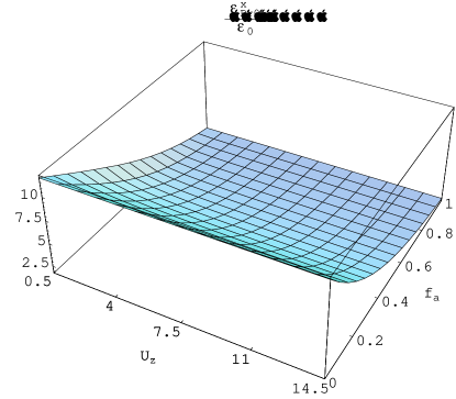
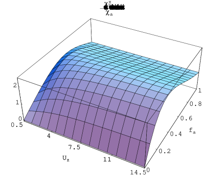
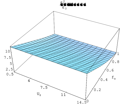
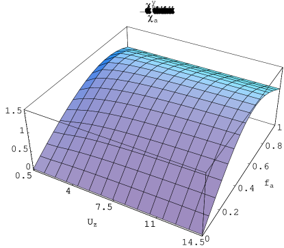
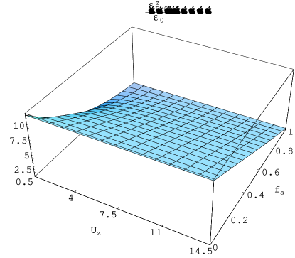
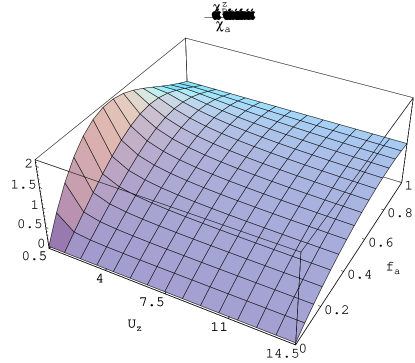
Figure 2: HCM relative linear permittivity and nonlinear susceptibility parameters calculated using the Bruggeman homogenization formalism. Component phase parameter values: $\epsilon_{a0}=2\epsilon_{\scriptscriptstyle 0}$, $\chi_{a}=9.07571\times 10^{-12}\epsilon_{\scriptscriptstyle 0}\,\mbox{m}^{2}\mbox{V}^{-2}$, $\epsilon_{b}\equiv\epsilon_{b0}=12\epsilon_{\scriptscriptstyle 0}$, $U_{x}=1$ and $U_{y}=3$.

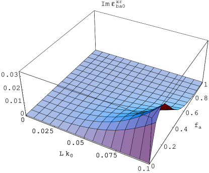
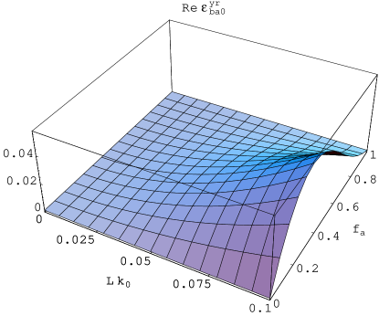
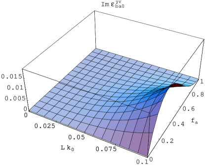
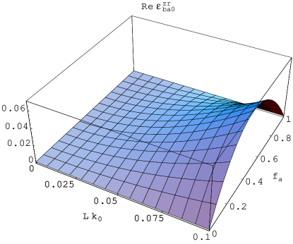
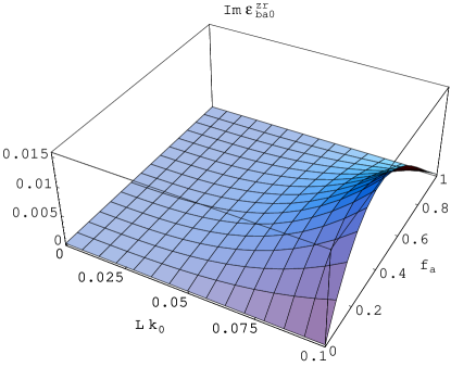
Figure 3: Real and imaginary parts of the HCM linear permittivity parameters calculated using the SPFT homogenization formalism. Component phase parameter values: $\epsilon_{a0}=2\epsilon_{\scriptscriptstyle 0}$, $\chi_{a}=9.07571\times 10^{-12}\epsilon_{\scriptscriptstyle 0}\,\mbox{m}^{2}\mbox{V}^{-2}$, $\epsilon_{b}\equiv\epsilon_{b0}=12\epsilon_{\scriptscriptstyle 0}$, $U_{x}=1$, $U_{y}=3$ and $U_{z}=15$.

The SPFT estimates of the HCM relative linear constitutive parameters $\epsilon^{xr,yr,zr}_{ba0}$ and nonlinear constitutive parameters $\chi^{xr,yr,zr}_{ba}$ are plotted in figures 2 and 3, respectively, as functions of $f_{a}$ and $k_{0}L$. Significant differences are clear between the Bruggeman-estimated values and the SPFT-estimated values: The SPFT estimates of linear constitutive parameters provide an additive correction to the corresponding Bruggeman parameters, whereas for the nonlinear constitutive parameters the SPFT estimates provide a subtractive correction to the corresponding Bruggeman parameters. Furthermore, the magnitudes of these differences exhibit local maxima which occur at progressively higher values of $f_{a}$ as one compares the constitutive parameter components aligned with the $x$, $y$ and $z$ coordinate axes, respectively. This trend holds for both the real and the imaginary parts of both the linear permittivity and the nonlinear susceptibility parameters. However, it is less pronounced for the nonlinear constitutive parameters.

Coherent interactions between scattering centres enclosed within a region of linear dimensions $L$ are accommodated in the bilocally-approximated SPFT via the two-point covariance function (5) (see figure 1). Thus, since neither component phase $a$ nor component phase $b$ is dissipative, the nonzero imaginary parts of the SPFT constititutive parameters in figures 2 and 3 are attributable entirely to scattering losses. Furthermore, the magnitudes of the imaginary parts of the constitutive parameters are observed in figures 2 and 3 to increase as $L$ increases, due to the actions of greater numbers of scattering centres becoming correlated.

5 Concluding remarks

The bilocally-approximated SPFT for weakly nonlinear isotropic HCMs, based on spherical particulate geometry, has been recently established [16, 17, 24]. In the present study we further advance the theory through considering anisotropic, cubically nonlinear HCMs, arising from isotropic component phases with ellipsoidal particulate geometries. Significant differences between the bilocally-approximated SPFT (i.e., second-order theory) and the Bruggeman homogenization formalism (i.e., zeroth-order theory) — which depend upon the underlying particulate geometry — have emerged. In particular, nonlinearity enhancement is predicted to a lesser degree with the SPFT than with the Bruggeman homogenization formalism. The importance of taking into account the distributional statistics of the HCM component phases is thereby further emphasized.

Acknowledgements: This study was partially carried out during a visit to the Department of Engineering Science and Mechanics at Pennsylvania State University. The author acknowledges the financial support of The Carnegie Trust for the Universities of Scotland and thanks Professors Akhlesh Lakhtakia (Pennsylvania State University) for suggesting the present study and Werner S. Weiglhofer (University of Glasgow) for numerous discussions regarding homogenization.

Appendix

Consider the principal value integral term $\underline{\underline{W}}$ (33) which was expressed as the sum $\underline{\underline{W}}_{\,0}+\underline{\underline{W}}_{\,1}\,|\,{\bf E}_{\,HCM}\,|^{2}$ in §3. Here we develop expressions for the linear component $\underline{\underline{W}}_{\,0}$ and the nonlinear component $\underline{\underline{W}}_{\,1}$, appropriate to the homogenization scenario of §2.

Let us begin with the following straightforward specialization of the evaluation of $\underline{\underline{W}}$ for bianisotropic HCMs [21, 22]

$$\underline{\underline{W}}=\frac{f_{a}f_{b}}{2\pi^{2}\,i\omega}\int d^{3}{\bf q}\;\;\frac{(q/\omega)^{2}\,\underline{\underline{\alpha}}+\underline{\underline{\beta}}}{(q/\omega)^{4}\,t_{C}+(q/\omega)^{2}\,t_{B}+t_{A}}\,\left(\,\frac{\sin qL}{q}-L\cos qL\,\right)\,.$$ (45)

For the weakly nonlinear homogenization outlined in §2, the scalar terms $t_{A}$, $t_{B}$ and $t_{C}$ in (45), along with their linear and nonlinear decompositions, are given by

$$t_{A}=\mu_{\scriptscriptstyle 0}^{3}\,\det\left[\,\underline{\underline{\epsilon}}_{\,Br}\,\right]=t_{A0}+t_{A1}\,|\,{\bf E}_{\,HCM}\,|^{2},$$ (46)

$$t_{B}=\mu_{\scriptscriptstyle 0}^{2}\,\left\{\mbox{tr}\left[\,\underline{\underline{\epsilon}}^{adj}_{\,Br}\mbox{ \tiny{${}^{\bullet}$} }\underline{\underline{A}}\,\right]-\left(\,\mbox{tr}\left[\,\underline{\underline{\epsilon}}^{adj}_{\,Br}\,\right]\,\mbox{tr}\left[\,\underline{\underline{A}}\,\right]\,\right)\,\right\}=t_{B0}+t_{B1}\,|\,{\bf E}_{\,HCM}\,|^{2},$$ (47)

$$t_{C}=\mu_{\scriptscriptstyle 0}\,\mbox{tr}\left[\,\underline{\underline{A}}\,\right]\,\mbox{tr}\left[\,\underline{\underline{\epsilon}}_{Br}\mbox{ \tiny{${}^{\bullet}$} }\underline{\underline{A}}\,\right]=t_{C0}+t_{C1}\,|\,{\bf E}_{\,HCM}\,|^{2}\,,$$ (48)

wherein

$$t_{A0}=\mu_{\scriptscriptstyle 0}^{3}\,\det\left[\,\underline{\underline{\epsilon}}_{\,Br0}\,\right]\,,\hskip 28.45274ptt_{A1}=\mu_{\scriptscriptstyle 0}^{3}\,\left(\,\chi^{x}_{Br}\,\epsilon^{y}_{Br0}\,\epsilon^{z}_{Br0}+\epsilon^{x}_{Br0}\,\chi^{y}_{Br}\,\epsilon^{z}_{Br0}+\epsilon^{x}_{Br0}\,\epsilon^{y}_{Br0}\,\chi^{z}_{Br}\,\right)\,,\quad$$ (49)

$$t_{B0}=\mu_{\scriptscriptstyle 0}^{2}\,\left\{\mbox{tr}\left[\,\underline{\underline{\epsilon}}^{adj}_{\,Br0}\mbox{ \tiny{${}^{\bullet}$} }\underline{\underline{A}}\,\right]-\left(\,\mbox{tr}\left[\,\underline{\underline{\epsilon}}^{adj}_{\,Br0}\,\right]\,\mbox{tr}\left[\,\underline{\underline{A}}\,\right]\,\right)\,\right\}\,,$$ (50)

$$t_{B1}=\mu_{\scriptscriptstyle 0}^{2}\,\left\{\mbox{tr}\left[\,\underline{\underline{\Upsilon}}\mbox{ \tiny{${}^{\bullet}$} }\underline{\underline{A}}\,\right]-\left(\,\mbox{tr}\left[\,\underline{\underline{\Upsilon}}\,\right]\,\mbox{tr}\left[\,\underline{\underline{A}}\,\right]\,\right)\,\right\}\,,$$ (51)

$$\underline{\underline{\Upsilon}}=\mbox{diag}\,\left(\,\chi^{y}_{Br}\,\epsilon^{z}_{Br0}+\epsilon^{y}_{Br0}\,\chi^{z}_{Br},\,\chi^{z}_{Br}\,\epsilon^{x}_{Br0}+\epsilon^{z}_{Br0}\,\chi^{x}_{Br},\,\chi^{x}_{Br}\,\epsilon^{y}_{Br0}+\epsilon^{x}_{Br0}\,\chi^{y}_{Br}\,\right)\,,$$ (52)

$$t_{C0}=\mu_{\scriptscriptstyle 0}\,\mbox{tr}\left[\,\underline{\underline{A}}\,\right]\,\mbox{tr}\left[\,\underline{\underline{\epsilon}}_{Br0}\mbox{ \tiny{${}^{\bullet}$} }\underline{\underline{A}}\,\right]\,,\hskip 42.67912ptt_{C1}=\mu_{\scriptscriptstyle 0}\,\mbox{tr}\left[\,\underline{\underline{A}}\,\right]\,\mbox{tr}\left[\,\underline{\underline{\chi}}_{Br}\mbox{ \tiny{${}^{\bullet}$} }\underline{\underline{A}}\,\right]\,.$$ (53)

Similarly, the dyadic quantities $\underline{\underline{\alpha}}$ and $\beta$ in (45), along with their linear and nonlinear decompositions, are given by

$$\underline{\underline{\alpha}}=\mu_{\scriptscriptstyle 0}^{2}\,\left[\,\left(2\,\underline{\underline{\epsilon}}_{\,Br}-\mbox{tr}\left[\,\underline{\underline{\epsilon}}_{\,Br}\,\right]\,\underline{\underline{I}}\,\right)\mbox{ \tiny{${}^{\bullet}$} }\underline{\underline{A}}-\mbox{tr}\left[\,\underline{\underline{\epsilon}}_{\,Br}\mbox{ \tiny{${}^{\bullet}$} }\underline{\underline{A}}\,\right]\,\underline{\underline{I}}\,\right]-\mu_{\scriptscriptstyle 0}\,\frac{t_{B}}{t_{C}}\,\mbox{tr}\left[\,\underline{\underline{A}}\,\right]\,\underline{\underline{A}}=\underline{\underline{\alpha}}_{\,0}+\underline{\underline{\alpha}}_{\,1}\,|\,{\bf E}_{\,HCM}\,|^{2},$$

(54)

$$\underline{\underline{\beta}}=\mu_{\scriptscriptstyle 0}^{3}\,\underline{\underline{\epsilon}}^{adj}_{\,Br}-\mu_{\scriptscriptstyle 0}\,\frac{t_{A}}{t_{C}}\,\mbox{tr}\left[\,\underline{\underline{A}}\,\right]\,\underline{\underline{A}}=\underline{\underline{\beta}}_{\,0}+\underline{\underline{\beta}}_{\,1}\,|\,{\bf E}_{\,HCM}\,|^{2},$$ (55)

with

$$\underline{\underline{\alpha}}_{\,0}=\mu_{\scriptscriptstyle 0}^{2}\,\left[\,\left(2\,\underline{\underline{\epsilon}}_{\,Br0}-\mbox{tr}\left[\,\underline{\underline{\epsilon}}_{\,Br0}\,\right]\,\underline{\underline{I}}\,\right)\mbox{ \tiny{${}^{\bullet}$} }\underline{\underline{A}}-\mbox{tr}\left[\,\underline{\underline{\epsilon}}_{\,Br0}\mbox{ \tiny{${}^{\bullet}$} }\underline{\underline{A}}\,\right]\,\underline{\underline{I}}\,\right]-\mu_{\scriptscriptstyle 0}\,\frac{t_{B0}}{t_{C0}}\,\mbox{tr}\left[\,\underline{\underline{A}}\,\right]\,\underline{\underline{A}}\,,$$ (56)

$$\underline{\underline{\alpha}}_{\,1}=\mu_{\scriptscriptstyle 0}^{2}\,\left[\,\left(2\,\underline{\underline{\chi}}_{\,Br}-\mbox{tr}\left[\,\underline{\underline{\chi}}_{\,Br}\,\right]\,\underline{\underline{I}}\,\right)\mbox{ \tiny{${}^{\bullet}$} }\underline{\underline{A}}-\mbox{tr}\left[\,\underline{\underline{\chi}}_{\,Br}\mbox{ \tiny{${}^{\bullet}$} }\underline{\underline{A}}\,\right]\,\underline{\underline{I}}\,\right]-\mu_{\scriptscriptstyle 0}\,\frac{t_{B1}-\left(t_{B0}/t_{C0}\right)t_{C1}}{t_{C0}}\,\mbox{tr}\left[\,\underline{\underline{A}}\,\right]\,\underline{\underline{A}}\,,$$

(57)

$$\underline{\underline{\beta}}_{\,0}=\mu_{\scriptscriptstyle 0}^{3}\,\underline{\underline{\epsilon}}^{adj}_{\,Br0}-\mu_{\scriptscriptstyle 0}\frac{t_{A0}}{t_{C0}}\,\mbox{tr}\left[\,\underline{\underline{A}}\,\right]\,\underline{\underline{A}}\,,\hskip 28.45274pt\underline{\underline{\beta}}_{\,1}=\mu_{\scriptscriptstyle 0}^{3}\,\underline{\underline{\Upsilon}}-\mu_{\scriptscriptstyle 0}\,\frac{t_{A1}-\left(t_{A0}/t_{C0}\right)t_{C1}}{t_{C0}}\,\mbox{tr}\left[\,\underline{\underline{A}}\,\right]\,\underline{\underline{A}}\,.$$ (58)

In the long-wavelength regime, i.e., $|\,d_{\pm}\,|\ll 1$ , the application of residue calculus to (45) delivers

$$\underline{\underline{W}}=\frac{f_{a}f_{b}\,\omega}{4\pi i}\int^{2\pi}_{0}d\phi\int^{\pi}_{0}d\theta\;\;\frac{\sin\theta}{3\,\Delta}\left\{\,\frac{1}{\omega^{2}}\left[\,\frac{3}{2}\,\left(\,d^{2}_{+}-d^{2}_{-}\,\right)+i\left(\,d^{3}_{+}-d^{3}_{-}\,\right)\right]\underline{\underline{\alpha}}+i\,\left(\,\frac{d^{3}_{+}}{\kappa_{+}}-\frac{d^{3}_{-}}{\kappa_{-}}\,\right)\underline{\underline{\beta}}\,\right\}\,,$$

where we have introduced

$$\Delta=\sqrt{t^{2}_{B}-4t_{A}t_{C}}=\Delta_{0}+\Delta_{1}\,|\,{\bf E}_{\,HCM}\,|^{2},$$ (60)

$$\kappa_{\pm}=\omega^{2}\,\frac{-t_{B}\pm\Delta}{2\,t_{C}}=\kappa_{0\pm}+\kappa_{1\pm}\,|\,{\bf E}_{\,HCM}\,|^{2},$$ (61)

$$d_{\pm}=L\sqrt{\kappa_{\pm}}=d_{0\pm}+d_{1\pm}\,|\,{\bf E}_{\,HCM}\,|^{2},$$ (62)

with linear and nonlinear parts

$$\Delta_{0}=\sqrt{t^{2}_{B0}-4t_{A0}t_{C0}}\,,\hskip 42.67912pt\Delta_{1}=\frac{t_{B0}t_{B1}-2\,\left(\,t_{A1}t_{C0}+t_{A0}t_{C1}\,\right)}{\Delta_{0}}\,,$$ (63)

$$\kappa_{0\pm}=\omega^{2}\,\frac{-t_{B0}\pm\Delta_{0}}{2\,t_{C0}}\,,\hskip 42.67912pt\kappa_{1\pm}=\omega^{2}\,\frac{\left(\,-t_{B1}\pm\Delta_{1}\,\right)-2t_{C1}\,\left(\kappa_{0\pm}/\omega^{2}\right)}{2\,t_{C0}}\,,$$ (64)

$$d_{0\pm}=L\sqrt{\kappa_{0\pm}}\,,\hskip 71.13188ptd_{1\pm}=L\frac{\kappa_{1\pm}}{2\sqrt{\kappa_{0\pm}}}\,.$$ (65)

The linear and nonlinear components of $\underline{\underline{W}}$ are thereby given as

$$\underline{\underline{W}}_{\,0} = \frac{f_{a}f_{b}\,\omega}{4\pi i}\int^{2\pi}_{0}d\phi\int^{\pi}_{0}d\theta\;\;\frac{\sin\theta}{3\,\Delta_{0}}\left(\,\frac{\tau_{\alpha}}{\omega^{2}}\,\underline{\underline{\alpha}}_{\,0}+\tau_{\beta}\,\underline{\underline{\beta}}_{\,0}\,\right)\,,$$ (66)

and

$$\underline{\underline{W}}_{\,1} = \frac{f_{a}f_{b}\,\omega}{4\pi i}\int^{2\pi}_{0}d\phi\int^{\pi}_{0}d\theta\;\;\sin\theta\;\times$$ (67)

$$\Bigg{\{}\frac{1}{3\,\Delta_{0}}\Bigg{[}\,\frac{\tau_{\alpha}}{\omega^{2}}\,\underline{\underline{\alpha}}_{\,1}+\tau_{\beta}\,\underline{\underline{\beta}}_{\,1}+\frac{3}{\omega^{2}}\Big{[}d_{0+}d_{1+}\left(1+id_{0+}\right)-d_{0-}d_{1-}\left(1+id_{0-}\right)\Big{]}\underline{\underline{\alpha}}_{\,0}+$$

$$i\left[\frac{d^{3}_{0+}}{\kappa_{0+}}\left(\frac{3d_{1+}}{d_{0+}}-\frac{\kappa_{1+}}{\kappa_{0+}}\right)-\frac{d^{3}_{0-}}{\kappa_{0-}}\left(\frac{3d_{1-}}{d_{0-}}-\frac{\kappa_{1-}}{\kappa_{0-}}\right)\right]\underline{\underline{\beta}}_{\,0}\,\Bigg{]}-\frac{\Delta_{1}}{3\Delta^{2}_{0}}\left(\,\frac{\tau_{\alpha}}{\omega^{2}}\,\underline{\underline{\alpha}}_{\,0}+\tau_{\beta}\,\underline{\underline{\beta}}_{\,0}\,\right)\,\Bigg{\}}\,,\quad$$

respectively, where

$$\tau_{\alpha}=\frac{3}{2}\,\left(\,d^{2}_{0+}-d^{2}_{0-}\,\right)+i\left(\,d^{3}_{0+}-d^{3}_{0-}\,\right)\,,\hskip 42.67912pt\tau_{\beta}=i\,\left(\,\frac{d^{3}_{0+}}{\kappa_{0+}}-\frac{d^{3}_{0-}}{\kappa_{0-}}\,\right)\,.$$ (68)

The integrals (66) and (67) are straightforwardly evaluated by standard (e.g., Gaussian) numerical methods [34]. In the degenerate isotropic case $U_{x}=U_{y}=U_{z}$, the integrals (66) and (67) yield the analytic results of [17].

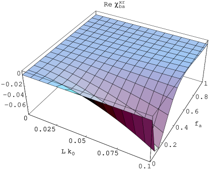
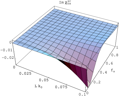
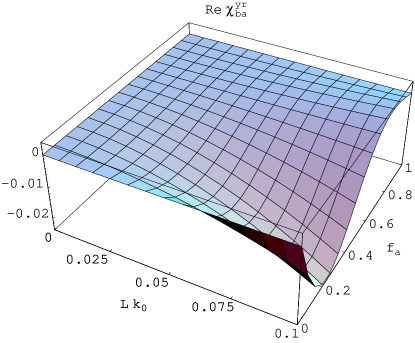
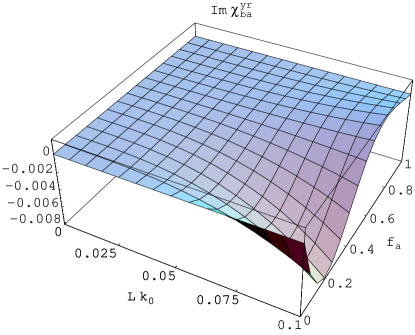
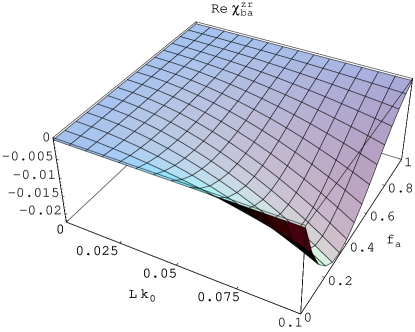
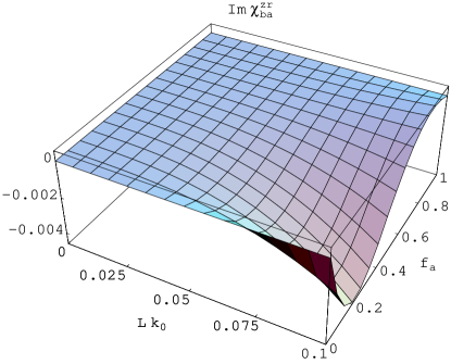
Figure 4: As figure 3 but for the HCM nonlinear susceptibility parameters.

References

• [1] Lakhtakia A (ed) 1996 Selected Papers on Linear Optical Composite Materials (Bellingham WA: SPIE Optical Engineering Press)
• [2] Beroual A, Brosseau C and Boudida A 2000 Permittivity of lossy heterostructures: effect of shape anisotropy J. Phys. D: Appl. Phys. 33 1969
• [3] Boyd R W, Gehr R J, Fischer G L and Sip J E 1996 Nonlinear optical properties of nanocomposite materials Pure Appl. Opt. 5 505
• [4] Michel B 2000 Recent developments in the homogenization of linear bianisotropic composite materials. In Electromagnetic fields in unconventional materials and structures O N Singh and A Lakhtakia (eds) (New York: John Wiley and Sons)
• [5] Mackay T G 2003 Homogenization of linear and nonlinear complex composite materials. In Introduction to Complex Mediums for Optics and Electromagnetics W S Weiglhofer and A Lakhtakia (eds) (Bellingham WA: SPIE Optical Engineering Press) In preparation
• [6] Ward L 1980 The Optical Constants of Bulk Materials and Films (Bristol: Adam Hilger)
• [7] Mackay T G and Weiglhofer W S 2001 Homogenization of biaxial composite materials: nondissipative dielectric properties Electromagnetics 21 15
• [8] Mackay T G and Weiglhofer W S 2000 Homogenization of biaxial composite materials: dissipative anisotropic properties J. Opt. A: Pure Appl. Opt. 2 426
• [9] Mackay T G and Weiglhofer W S 2001 Homogenization of biaxial composite materials: bianisotropic properties J. Opt. A: Pure Appl. Opt. 3 45
• [10] Mackay T G and Weiglhofer W S 2002 A review of homogenization studies for biaxial bianisotropic materials. In Advances in Metamaterials S Zoudhi, A H Sihvola and M Arsalane (eds) (Dordrecht, The Netherlands: Kluwer Academic Publishers), pp.211 – 228, 2002
• [11] Goncharenko A V, Popelnukh V V and Venger E F 2002 Effect of weak nonsphericity on linear and nonlinear optical properties of small particle composites J. Phys. D: Appl. Phys. 35 1833
• [12] Zeng X C, Bergman D J, Hui P M and Stroud D 1988 Effective-medium theory for weakly nonlinear composites Phys. Rev. B 38 10970
• [13] Tsang L and Kong J A 1981 Scattering of electromagnetic waves from random media with strong permittivity fluctuations Radio Sci. 16 303
• [14] Ryzhov Yu A and Tamoikin V V 1970 Radiation and propagation of electromagnetic waves in randomly inhomogeneous media Radiophys. Quantum Electron. 14 228
• [15] Frisch U 1970 Wave propagation in random media. In Probabilistic Methods in Applied Mathematics Vol. 1 A T Bharucha–Reid (ed) (London: Academic Press)
• [16] Lakhtakia A 2001 Application of strong permittivity fluctuation theory for isotropic, cubically nonlinear, composite mediums Opt. Commun. 192 145
• [17] Mackay T G, Lakhtakia A and Weiglhofer W S 2002 Homogenisation of isotropic, cubically nonlinear, composite mediums by the strong–permittivity–fluctuation theory: third–order considerations Opt. Commun. 204 219
• [18] Zhuck N P 1994 Strong–fluctuation theory for a mean electromagnetic field in a statistically homogeneous random medium with arbitrary anisotropy of electrical and statistical properties Phys. Rev. B 50 15636
• [19] Mackay T G, Lakhtakia A and Weiglhofer W S 2001 Homogenisation of similarly oriented, metallic, ellipsoidal inclusions using the bilocally approximated strong–property–fluctuation theory Opt. Commun. 107 89
• [20] Michel B and Lakhtakia A 1995 Strong–property–fluctuation theory for homogenizing chiral particulate composites Phys. Rev. E 51 5701
• [21] Mackay T G, Lakhtakia A and Weiglhofer W S 2000 Strong–property–fluctuation theory for homogenization of bianisotropic composites: formulation Phys. Rev. E 62 6052 Erratum 2001 63 049901(E)
• [22] Mackay T G, Lakhtakia A and Weiglhofer W S 2001 Ellipsoidal topology, orientation diversity and correlation length in bianisotropic composite mediums Arch. Elekron. Übertrag. 55 243
• [23] Mackay T G, Lakhtakia A and Weiglhofer W S 2001 Third–order implementation and convergence of the strong–property–fluctuation theory in electromagnetic homogenization Phys. Rev. E 64 066616
• [24] Mackay T G, Lakhtakia A and Weiglhofer W S 2002 Electromagnetic homogenization of cubically nonlinear, isotropic chiral composite mediums via the strong–property–fluctuation theory Department of Mathematics Preprint No. 02/24 , University of Glasgow
• [25] Boyd R W 1992 Nonlinear Optics (London: Academic Press)
• [26] Tsang L, Kong J A and Newton R W 1982 Application of strong fluctuation random medium theory to scattering of electromagnetic waves from a half–space of dielectric mixture IEEE Trans. Antennas Propagat. 30 292
• [27] Michel B 1997 A Fourier space approach to the pointwise singularity of an anisotropic dielectric medium Int. J. Appl. Electromagn. Mech. 8 219
• [28] Michel B and Weiglhofer W S 1997 Pointwise singularity of dyadic Green function in a general bianisotropic medium Arch. Elekron. Übertrag. 51 219 Erratum 1998 52 31
• [29] Weiglhofer W S 1998 Electromagnetic depolarization dyadics and elliptic integrals J. Phys. A: Math. Gen. 31 7191
• [30] Bohren C F and Huffman D R 1983 Absorption and Scattering of Light by Small Particles (New York: Wiley)
• [31] Lakhtakia M N and Lakhtakia A 2001 Anisotropic composite materials with intensity–dependent permittivity tensor: the Bruggeman approach Electromagnetics 21 129
• [32] Ashcroft N W and Mermin N D 1976 Solid State Physics (Philadelphia: Saunders College).
• [33] Liao H B, Xiao R F, Wang H, Wong K S and Wong G K L 1998 Large third-order optical nonlinearity in $\mbox{Au:TiO}_{2}$ composite films measured on a femtosecond time scale Appl. Phys. Lett. 72 1817
• [34] W H Press, B P Flannery, S A Teukolsky and W T Vetterling 1992 Numerical Recipes in Fortran 2nd Edition (Cambridge: Cambridge University Press)