Depolarization volume and correlation length in the homogenization of anisotropic dielectric composites

Tom G. Mackay111 Tel: +44 131 650 5058; fax: +44 131 650 6553; e–mail: T.Mackay@ed.ac.uk

School of Mathematics, University of Edinburgh,
James Clerk Maxwell Building, King’s Buildings, Edinburgh EH9 3JZ, United Kingdom.

Abstract

In conventional approaches to the homogenization of random particulate composites, both the distribution and size of the component phase particles are often inadequately taken into account. Commonly, the spatial distributions are characterized by volume fraction alone, while the electromagnetic response of each component particle is represented as a vanishingly small depolarization volume. The strong-permittivity-fluctuation theory (SPFT) provides an alternative approach to homogenization wherein a comprehensive description of distributional statistics of the component phases is accommodated. The bilocally-approximated SPFT is presented here for the anisotropic homogenized composite which arises from component phases comprising ellipsoidal particles. The distribution of the component phases is characterized by a two-point correlation function and its associated correlation length. Each component phase particle is represented as an ellipsoidal depolarization region of nonzero volume. The effects of depolarization volume and correlation length are investigated through considering representative numerical examples. It is demonstrated that both the spatial extent of the component phase particles and their spatial distributions are important factors in estimating coherent scattering losses of the macroscopic field.

Keywords: Strong-permittivity-fluctuation theory, anisotropy, ellipsoidal particles, Bruggeman formalism

PACS numbers: 83.80.Ab, 05.40.-a

1 Introduction

Consider the propagation of electromagnetic radiation through a composite medium comprising a random distribution of particles. Provided wavelengths are sufficiently long compared with the dimensions of the component particles, the composite may be regarded as an effectively homogenous medium. The estimation of the constitutive parameters of such a homogenized composite medium (HCM) is a matter of long-standing scientific and technological importance [1, 2]. Furthermore, recent advances relating to HCM-based metamaterials have promoted interest in this area and highlighted the necessity for accurate formalisms to estimate the constitutive parameters of complex HCMs [3].

The microstructural details of the component phases are often inadequately incorporated in homogenization formalisms. In particular, conventional approaches to homogenization, as exemplified by the widely-applied Maxwell Garnett and Bruggeman formalisms, generally involve simplistic treatments of the distributional statistics and sizes of the component phase particles [4]. It is noteworthy that both the Maxwell–Garnett and Bruggeman formalisms arise in the long–wavelength regime. The long–wavelength derivation of the Maxwell–Garnett formalism follows a from rigorous treatment of the singularity of the free–space dyadic Green function [5, 6]. The Bruggeman formalism emerges from the strong-permittivity-fluctuation theory (SPFT) under the long–wavelength approximation [7, 8].

The SPFT provides an alternative approach to homogenization in which a comprehensive description of the distributional statistics of the component phases is accommodated. Though the SPFT was originally developed for wave propagation in continuous random mediums [7, 8, 9, 10], it has more recently gained prominence in the homogenization of particulate composites [11, 12, 13, 14, 15]. Within the SPFT, estimates of the HCM constitutive parameters are calculated as successive refinements to the constitutive parameters of a homogenous comparison medium. Iterates are expressed in terms of correlation functions describing the spatial distribution of the component phases. Correlation functions of arbitrarily high order may be incorporated in principle, but the SPFT is usually implemented at the second order level, known as the bilocal approximation. A two-point correlation function and its associated correlation length characterize the component phase distributions for the second order SPFT. At lowest order (i.e., zeroth and first order), the SPFT estimate of HCM permittivity is identical to that of the Bruggeman homogenization formalism [2].

Depolarization dyadics are key ingredients in homogenization analyses as they characterize the electromagnetic field inside inclusions (i.e., component phase particles) embedded within a homogenous background. Commonly, the inclusion particles are treated as vanishingly small point-like entities; under this approximation, the corresponding depolarization dyadic is represented by the singularity of the associated dyadic Green function [16, 17]. Through neglecting the spatial extent of the inclusions, potentially important information is lost, particularly when coherent scattering losses are to be considered [18, 19]. It is noted that extended versions of both the Maxwell Garnett formalism [20, 21] and the Bruggeman formalism [20, 22] have been developed in which a nonzero volume is attributed to the component phase particles. However, these analyses apply only to isotropic HCMs and adopt a simplistic description of the distributional statistics of the component phases.

In the present study, the SPFT is presented for an anisotropic dielectric HCM. The analysis takes place within the frequency–domain, wherein dissipation is signalled by constitutive parameters having nonzero imaginary parts. The component phases are taken to consist of randomly distributed, ellipsoidal particles of nonzero volume. In Section 2, the depolarization dyadic appropriate to an ellipsoidal inclusion of linear dimensions proportional to the size parameter $\eta>0$, embedded within an anisotropic comparison medium, is developed. Details of the SPFT-based homogenization are presented in Section 3. In Section 4, the theoretical results are illustrated by representative numerical examples relating to both nondissipative and dissipative component phases. In particular, nondissipative component phases giving rise to dissipative HCMs — through radiative scattering loss from the macroscopic coherent field [23] — is highlighted. A few concluding remarks are provided in Section 5.

In the notation adopted, vector quantities are underlined whereas 3$\times$3 dyadics are double underlined. The inverse, adjoint, determinant and trace of a dyadic $\underline{\underline{M}}$ are denoted by $\underline{\underline{M}}^{-1}$, $\underline{\underline{M}}^{adj}$ , $\mbox{det}\,\left[\,\underline{\underline{M}}\,\right]$ and $\mbox{tr}\,\left[\,\underline{\underline{M}}\,\right]$, respectively. The identity dyadic is represented by $\,\underline{\underline{I}}\,$. All field–related quantities are implicitly functions of the angular frquency $\omega$. The permittivity and permeability of free space are denoted as $\epsilon_{\scriptscriptstyle 0}$ and $\mu_{\scriptscriptstyle 0}$, respectively; the free-space wavenumber is $k_{\scriptscriptstyle 0}=\omega\sqrt{\epsilon_{\scriptscriptstyle 0}\mu_{\scriptscriptstyle 0}}$. The real and imaginary parts of complex-valued quantities are represented by $\mbox{Re}\,\left(\mbox{ \tiny{${}^{\bullet}$} }\right)$ and $\mbox{Im}\,\left(\mbox{ \tiny{${}^{\bullet}$} }\right)$, respectively.

2 Depolarization

Let us consider an ellipsoidal inclusion of volume $V^{\eta}_{e}$, orientated with its principal axes lying along the Cartesian $x,y,z$ axes. The ellipsoidal surface of $V^{\eta}_{e}$ is parameterized by

$$\underline{r}_{\,e}(\theta,\phi)=\eta\,\underline{\underline{U}}\mbox{ \tiny{${}^{\bullet}$} }\underline{\hat{r}}\,(\theta,\phi),$$ (1)

where $\underline{\hat{r}}\,(\theta,\phi)$ is the radial unit vector specified by the spherical polar coordinates $\theta$ and $\phi$. The diagonal shape dyadic

$$\underline{\underline{U}}=\frac{1}{\sqrt[3]{U_{x}U_{y}U_{z}}}\;\mbox{diag}(U_{x},U_{y},U_{z}),\hskip 71.13188pt(U_{x},U_{y},U_{z}>0),$$ (2)

maps the spherical region $V^{\eta}$ of radius $\eta$ onto the ellipsoidal region $V^{\eta}_{e}$. The linear dimensions of the ellipsoidal inclusion, as determined by $\eta$, are assumed to be sufficiently small that the electromagnetic long-wavelength regime pertains, but not vanishingly small.

Suppose the ellipsoidal inclusion is embedded within a homogenous comparison medium. In consonance with the shape dyadic (2), the comparison medium is taken as an anisotropic dielectric medium characterized by the diagonal permittivity dyadic $\underline{\underline{\epsilon}}_{\,cm}$ with principal axes aligned with those of $\underline{\underline{U}}$. We remark that $\underline{\underline{\epsilon}}_{\,cm}$, being established in the frequency–domain, is implicitly a fuction of $\omega$. The electromagnetic response of the ellipsoidal inclusion is provided by the depolarization dyadic

$$\underline{\underline{D}}=\int_{V^{\eta}_{e}}\,\underline{\underline{G}}_{\,cm}(\underline{r})\;d^{3}\underline{r}\,=\int_{V^{\eta}}\,\underline{\underline{G}}_{\,cm}(\underline{\underline{U}}\mbox{ \tiny{${}^{\bullet}$} }\underline{r})\;d^{3}\underline{r}\,.$$ (3)

Herein, $\underline{\underline{G}}_{\,cm}(\underline{r})$ is the dyadic Green function of the comparison medium which satisfies the nonhomogenous vector Helmholtz equation

$$\left(\nabla\times\nabla\times\underline{\underline{I}}-\omega^{2}\mu_{\scriptscriptstyle 0}\,\underline{\underline{\epsilon}}_{\,cm}\right)\mbox{ \tiny{${}^{\bullet}$} }\underline{\underline{G}}_{\,cm}(\underline{r}-\underline{r}^{\prime})=i\omega\mu_{\scriptscriptstyle 0}\delta\left(\underline{r}-\underline{r}^{\prime}\right)\underline{\underline{I}}\,.$$ (4)

Explicit representations of Green functions are not generally available for anisotropic mediums [24]. However, it suffices for our present purposes to consider the Fourier transform of $\underline{\underline{G}}_{\,cm}(\underline{r})$, namely

$$\underline{\underline{\tilde{G}}}_{\,cm}(\underline{q})=\int_{\underline{r}}\underline{\underline{G}}_{\,cm}(\underline{r})\,\exp(-i\underline{q}\mbox{ \tiny{${}^{\bullet}$} }\underline{r})\;d^{3}\underline{r}\,.$$ (5)

Taking the Fourier transform of equation (4) delivers $\underline{\underline{\tilde{G}}}_{\,cm}(\underline{q})$ as

$$\underline{\underline{\tilde{G}}}_{\,cm}(\underline{q})=-i\omega\mu_{\scriptscriptstyle 0}\left(\underline{q}\times\underline{q}\times\underline{\underline{I}}+\omega^{2}\mu_{\scriptscriptstyle 0}\,\underline{\underline{\epsilon}}_{\,cm}\right)^{-1}.$$ (6)

Thereby, equation (3) yields [16, 17]

$\displaystyle\underline{\underline{D}}$ $\displaystyle=$ $\displaystyle\frac{\eta}{2\pi^{2}}\,\int_{\underline{q}}\frac{1}{q^{2}}\,\left(\frac{\sin(q\eta)}{q\eta}-\cos(q\eta)\right)\,\underline{\underline{\tilde{G}}}_{\,cm}(\underline{\underline{U}}^{-1}\mbox{ \tiny{${}^{\bullet}$} }\underline{q})\;d^{3}\underline{q}\,.$ (7)

In order to consider the depolarization of an inclusion of nonzero volume, we express $\underline{\underline{D}}$ as the sum

$$\underline{\underline{D}}=\underline{\underline{D}}^{\eta}+\underline{\underline{D}}^{0}\,$$ (8)

where

$\displaystyle\underline{\underline{D}}^{\eta}=\frac{\eta}{2\pi^{2}}\,\int_{\underline{q}}\frac{1}{q^{2}}\,\left(\frac{\sin(q\eta)}{q\eta}-\cos(q\eta)\right)\,\underline{\underline{\tilde{G}}}^{\eta}_{\,cm}(\underline{\underline{U}}^{-1}\mbox{ \tiny{${}^{\bullet}$} }\underline{q})\;d^{3}\underline{q}\,,$ (9)
$\displaystyle\underline{\underline{D}}^{0}=\frac{\eta}{2\pi^{2}}\,\int_{\underline{q}}\frac{1}{q^{2}}\,\left(\frac{\sin(q\eta)}{q\eta}-\cos(q\eta)\right)\,\underline{\underline{\tilde{G}}}^{\infty}_{\,cm}(\underline{\underline{U}}^{-1}\mbox{ \tiny{${}^{\bullet}$} }\hat{\underline{q}})\;d^{3}\underline{q}\,,$ (10)

with

$\displaystyle\underline{\underline{\tilde{\bf G}}}^{\eta}_{\,cm}(\underline{\underline{U}}^{-1}\mbox{ \tiny{${}^{\bullet}$} }\underline{q})$ $\displaystyle=$ $\displaystyle\underline{\underline{\tilde{\bf G}}}_{\,cm}(\underline{\underline{U}}^{-1}\mbox{ \tiny{${}^{\bullet}$} }\underline{q})-\underline{\underline{\tilde{\bf G}}}^{\infty}_{\,cm}(\underline{\underline{U}}^{-1}\mbox{ \tiny{${}^{\bullet}$} }\hat{\underline{q}})\,,$ (11)
$\displaystyle\underline{\underline{\tilde{\bf G}}}^{\infty}_{\,cm}(\underline{\underline{U}}^{-1}\mbox{ \tiny{${}^{\bullet}$} }\hat{\underline{q}})$ $\displaystyle=$ $\displaystyle\lim_{q\rightarrow\infty}\;\underline{\underline{\tilde{\bf G}}}_{\,cm}(\underline{\underline{U}}^{-1}\mbox{ \tiny{${}^{\bullet}$} }\underline{q}).$ (12)

Thus, the dyadic $\underline{\underline{D}}^{0}$ represents the depolarization contribution arising from the vanishingly small region $\displaystyle{\lim_{\eta\rightarrow 0}}V^{\eta}_{e}$, whereas the dyadic $\underline{\underline{D}}^{\eta}$ provides the depolarization contribution arising from the region of nonzero volume $\left(V^{\eta}_{e}-\displaystyle{\lim_{\eta\rightarrow 0}}V^{\eta}_{e}\right)$. In homogenization studies, it is common practice to neglect $\underline{\underline{D}}^{\eta}$ and assume that the depolarization dyadic is given by $\underline{\underline{D}}^{0}$ alone [2]. However, studies of isotropic HCMs have emphasized the importance of the nonzero spatial extent of depolarization regions [18, 19, 20, 21, 22].

The properties of depolarization dyadics associated with vanishingly small inclusions have been widely investigated: the volume integral (10) simplifies to the $\eta$–independent surface integral [16, 17]

$\displaystyle\underline{\underline{D}}^{0}$ $\displaystyle=$ $\displaystyle\frac{1}{4\pi i\omega}\,\int^{2\pi}_{0}\;d\phi\,\int^{\pi}_{0}\;d\theta\;\sin\theta\,\left(\,\frac{1}{\mbox{tr}\left(\,\underline{\underline{\epsilon}}_{\,cm}\mbox{ \tiny{${}^{\bullet}$} }\underline{\underline{A}}\,\right)}\,\underline{\underline{A}}\,\right)\,,$ (13)

where

$$\underline{\underline{A}}=\mbox{diag}\,\left(\,\frac{\sin^{2}\theta\,\cos^{2}\phi}{U^{2}_{x}},\,\frac{\sin^{2}\theta\,\sin^{2}\phi}{U^{2}_{y}},\,\frac{\cos^{2}\theta}{U^{2}_{z}}\,\right)\,.$$ (14)

Furthermore, the integrations of (13) reduce to elliptic function representations [25]. In the case of spheroidal inclusion geometries, hyperbolic functions provide an evaluation of $\underline{\underline{D}}^{0}$ [16], while for the degenerate isotropic case $U_{x}=U_{y}=U_{z}$ the well-known result $\underline{\underline{D}}^{0}=\left(1/3i\omega\right)\underline{\underline{\epsilon}}^{-1}_{\,cm}$ emerges [26].

We focus attention on $\underline{\underline{D}}^{\eta}$. By analogy with an equivalent integration which arises within the strong–permittivity–fluctuation theory [27], the application of residue calculus to (9) provides

$\displaystyle\underline{\underline{D}}^{\eta}=\frac{1}{4\pi i\omega}\,\underline{\underline{W}}(\eta),$ (15)

where the dyadic function $\underline{\underline{W}}(\eta)$ has the surface integral representation

$\displaystyle\underline{\underline{W}}(\eta)=\eta^{3}\int^{2\pi}_{0}d\phi\int^{\pi}_{0}d\theta\;\;\frac{\sin\theta}{3\,\Delta}\left\{\,\left[\,\frac{3\left(\kappa_{+}-\kappa_{-}\right)}{2\eta}+i\left(\kappa^{\frac{3}{2}}_{+}-\kappa^{\frac{3}{2}}_{-}\right)\right]\underline{\underline{\alpha}}+i\omega^{2}\mu_{\scriptscriptstyle 0}\,\left(\kappa^{\frac{1}{2}}_{+}-\kappa^{\frac{1}{2}}_{-}\right)\underline{\underline{\beta}}\,\right\},$
(16)

with

$\displaystyle\underline{\underline{\alpha}}=\left[2\,\underline{\underline{\epsilon}}_{\,cm}-\mbox{tr}\left(\,\underline{\underline{\epsilon}}_{\,cm}\,\right)\,\underline{\underline{I}}\,\right]\mbox{ \tiny{${}^{\bullet}$} }\underline{\underline{A}}-\mbox{tr}\left(\,\underline{\underline{\epsilon}}_{\,cm}\mbox{ \tiny{${}^{\bullet}$} }\underline{\underline{A}}\,\right)\,\underline{\underline{I}}\,-\,\frac{\mbox{tr}\left(\,\underline{\underline{\epsilon}}^{adj}_{\,cm}\mbox{ \tiny{${}^{\bullet}$} }\underline{\underline{A}}\,\right)-\left[\,\mbox{tr}\left(\,\underline{\underline{\epsilon}}^{adj}_{\,cm}\,\right)\,\mbox{tr}\left(\,\underline{\underline{A}}\,\right)\,\right]}{\mbox{tr}\left(\,\underline{\underline{\epsilon}}_{\,cm}\mbox{ \tiny{${}^{\bullet}$} }\underline{\underline{A}}\,\right)}\,\underline{\underline{A}}\,$
(17)
$\displaystyle\underline{\underline{\beta}}=\underline{\underline{\epsilon}}^{adj}_{\,cm}-\frac{\det\left(\,\underline{\underline{\epsilon}}_{\,cm}\,\right)}{\mbox{tr}\left(\,\underline{\underline{\epsilon}}_{\,cm}\mbox{ \tiny{${}^{\bullet}$} }\underline{\underline{A}}\,\right)}\,\underline{\underline{A}}\,,$ (18)
$\displaystyle\Delta=\left\{\left[\mbox{tr}\left(\,\underline{\underline{\epsilon}}^{adj}_{\,cm}\mbox{ \tiny{${}^{\bullet}$} }\underline{\underline{A}}\,\right)-\mbox{tr}\left(\,\underline{\underline{\epsilon}}^{adj}_{\,cm}\,\right)\,\mbox{tr}\left(\,\underline{\underline{A}}\,\right)\,\right]^{2}-4\det\left(\,\underline{\underline{\epsilon}}_{\,cm}\,\right)\mbox{tr}\left(\,\underline{\underline{A}}\,\right)\,\mbox{tr}\left(\,\underline{\underline{\epsilon}}_{\,cm}\mbox{ \tiny{${}^{\bullet}$} }\underline{\underline{A}}\,\right)\right\}^{\frac{1}{2}},$ (19)
$\displaystyle\kappa_{\pm}=\mu_{\scriptscriptstyle 0}\omega^{2}\frac{\left[\,\mbox{tr}\left(\,\underline{\underline{\epsilon}}^{adj}_{\,cm}\,\right)\,\mbox{tr}\left(\,\underline{\underline{A}}\,\right)\,\right]-\mbox{tr}\left(\,\underline{\underline{\epsilon}}^{adj}_{\,cm}\mbox{ \tiny{${}^{\bullet}$} }\underline{\underline{A}}\,\right)\pm\Delta}{2\,\mbox{tr}\left(\,\underline{\underline{A}}\,\right)\,\mbox{tr}\left(\,\underline{\underline{\epsilon}}_{\,cm}\mbox{ \tiny{${}^{\bullet}$} }\underline{\underline{A}}\,\right)}.$ (20)

The surface integrals of (13) and (16) are straightforwardly evaluated by standard numerical techniques [28].

3 Homogenization

The SPFT may be applied to estimate the constitutive parameters of HCMs. Let us consider the homogenization of a two–phase composite wherein the two component phases, labelled as $a$ and $b$, comprise ellipsoidal particles of shape specified by $\underline{\underline{U}}$ and linear dimensions specified by $\eta>0$. A random distribution of identically orientated particles is envisaged. The component phases $a$ and $b$ are taken to be isotropic dielectric mediums with permittivities $\epsilon_{a}$ and $\epsilon_{b}$, respectively.

The distributional statistics of the component phases are described in terms of moments of the characteristic functions

$$\Phi_{\ell}(\underline{r})=\left\{\begin{array}[]{ll}1,&\qquad\underline{r}\in V_{\,\ell},\\ &\qquad\qquad\qquad\qquad\qquad\qquad(\ell=a,b).\\ 0,&\qquad\underline{r}\not\in V_{\,\ell},\end{array}\right.$$ (21)

The volume fraction of phase $\ell$, namely $f_{\ell}$ , is given by the first statistical moment of $\Phi_{\ell}$ ; i.e., $\langle\,\Phi_{\ell}(\underline{r})\,\rangle=f_{\ell}$ . Clearly, $f_{a}+f_{b}=1$. The second statistical moment of $\Phi_{\ell}$ provides a two-point covariance function. We adopt the physically-motivated form [29]

$$\langle\,\Phi_{\ell}(\underline{r})\,\Phi_{\ell}(\underline{r}^{\prime})\,\rangle=\left\{\begin{array}[]{lll}\langle\,\Phi_{\ell}(\underline{r})\,\rangle\langle\Phi_{\ell}(\underline{r}^{\prime})\,\rangle\,,&&\hskip 28.45274pt|\,\underline{\underline{U}}^{-1}\mbox{ \tiny{${}^{\bullet}$} }\left(\underline{r}-\underline{r}^{\prime}\right)|>L\,,\\ &&\\ \langle\,\Phi_{\ell}(\underline{r})\,\rangle\,,&&\hskip 28.45274pt|\,\underline{\underline{U}}^{-1}\mbox{ \tiny{${}^{\bullet}$} }\left(\underline{r}-\underline{r}^{\prime}\right)|\leq L\,,\end{array}\right.$$ (22)

where $L>0$ is the correlation length. It is remarked that the specific form of the covariance function has little influence on SPFT estimates of HCM constititutive parameters [30].

The $n$th order SPFT estimate of the HCM permittivity, namely $\underline{\underline{\epsilon}}^{[n]}_{\,ab}$, is based upon the iterative refinement of the comparison medium permittivity, namely $\underline{\underline{\epsilon}}_{\,cm}$. To zeroth order and first order, the SPFT permittivity estimate is identical to the comparison medium permittivity [2]; i.e.,

$$\underline{\underline{\epsilon}}^{[0]}_{\,ab}=\underline{\underline{\epsilon}}^{[1]}_{\,ab}=\underline{\underline{\epsilon}}_{\,cm}.$$ (23)

The well–known Bruggeman homogenization formalism provides the estimate of $\underline{\underline{\epsilon}}_{\,cm}$ [14]. Thereby, $\underline{\underline{\epsilon}}_{\,cm}$ emerges through solving the nonlinear equations

$$f_{a}\,\underline{\underline{\chi}}_{\,a}+f_{b}\,\underline{\underline{\chi}}_{\,b}=\underline{\underline{0}}\,,$$ (24)

wherein the polarization dyadics

$$\underline{\underline{\chi}}_{\,\ell}=-i\,\omega\,\left(\,\epsilon_{\ell}\,\underline{\underline{I}}-\underline{\underline{\epsilon}}_{\,cm}\,\right)\mbox{ \tiny{${}^{\bullet}$} }\underline{\underline{\Gamma}}^{-1}_{\,\ell}\,,\hskip 85.35826pt(\ell=a,b),$$ (25)

are dependent upon the inclusion size parameter $\eta$ via

$$\underline{\underline{\Gamma}}_{\,\ell}=\left[\,\underline{\underline{I}}+i\omega\,\underline{\underline{D}}\mbox{ \tiny{${}^{\bullet}$} }\left(\,\epsilon_{\ell}\,\underline{\underline{I}}-\underline{\underline{\epsilon}}_{\,cm}\,\right)\,\right]\,.$$ (26)

Recursive procedures generate the $p$th iterate of $\underline{\underline{\epsilon}}_{\,cm}$ as

$$\underline{\underline{\epsilon}}_{\,cm}[p]=\mathcal{T}\,\left\{\,\underline{\underline{\epsilon}}_{\,cm}\,[p-1]\,\right\},$$ (27)

with the operator $\mathcal{T}$ being defined by

$\displaystyle\mathcal{T}\,\left\{\,\underline{\underline{\epsilon}}_{\,cm}\,\right\}$ $\displaystyle=$ $\displaystyle\left(\,f_{a}\,\epsilon_{a}\,\underline{\underline{\Gamma}}^{-1}_{\,a}+f_{b}\,\epsilon_{b}\,\underline{\underline{\Gamma}}^{-1}_{\,b}\,\right)\mbox{ \tiny{${}^{\bullet}$} }\left(\,f_{a}\,\underline{\underline{\Gamma}}^{-1}_{\,a}+f_{b}\,\underline{\underline{\Gamma}}^{-1}_{\,b}\,\right)^{-1}\,.$ (28)

The SPFT is most widely implemented at the second order level — known as the bilocal approximation — which provides the following estimate of the HCM permittivity dyadic [14]

$$\underline{\underline{\epsilon}}^{[2]}_{\,ab}=\underline{\underline{\epsilon}}_{\,cm}-\frac{1}{i\,\omega}\,\left(\,\underline{\underline{I}}+\underline{\underline{\Sigma}}\mbox{ \tiny{${}^{\bullet}$} }\underline{\underline{D}}\,\right)^{-1}\mbox{ \tiny{${}^{\bullet}$} }\underline{\underline{\Sigma}}\,.$$ (29)

Thus, the inclusion size parameter $\eta$ influences $\underline{\underline{\epsilon}}^{[2]}_{\,ab}$ directly through the depolarization dyadic $\underline{\underline{D}}$ and indirectly through the mass operator [9] dyadic term

$$\underline{\underline{\Sigma}}=\frac{f_{a}f_{b}}{4\pi i\omega}\left(\,\underline{\underline{\chi}}_{\,a}-\underline{\underline{\chi}}_{\,b}\,\right)\mbox{ \tiny{${}^{\bullet}$} }\underline{\underline{W}}(L)\mbox{ \tiny{${}^{\bullet}$} }\left(\,\underline{\underline{\chi}}_{\,a}-\underline{\underline{\chi}}_{\,b}\,\right).$$ (30)

Notice that the correlation length $L$ — which plays a key role in the second order SPFT — is not relevant to the zeroth order SPFT.

4 Numerical studies

We investigate the theoretical results presented in Sections 2 and 3 by means of representative numerical studies. To highlight the particular effects of depolarization volume and correlation length, it is expedient to begin with a study of HCMs arising from nondissipative component mediums (i.e., $\epsilon_{a,b}\in\mathbb{R}$) before proceeding to consider HCMs arising from dissipative component mediums (i.e., $\epsilon_{a,b}\in\mathbb{C}$ with $\mbox{Im}\,\left(\epsilon_{a,b}\right)>0$). However, we note that caution should be exercised when applying the SPFT and Bruggeman formalism to weakly dissipative HCMs where $\mbox{Re}\,\left(\epsilon_{a}\right)$ and $\mbox{Re}\,\left(\epsilon_{b}\right)$ have opposite signs [31]. For all calculations reported here, the angular frequency $\omega$ is fixed at $2\pi\times 10^{10}\;\mbox{rad s}^{-1}$.

4.1 Nondissipative component phases

Consider, for example, the HCM which arises from the nondissipative component phases specified by the permittivities and shape parameters

$$\left.\begin{array}[]{lll}\epsilon_{a}=2\epsilon_{\scriptscriptstyle 0},&\epsilon_{b}=12\epsilon_{\scriptscriptstyle 0}&\\ U_{x}=1,&U_{y}=3,&U_{z}=15\end{array}\right\}.$$ (31)

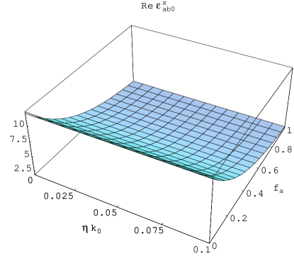
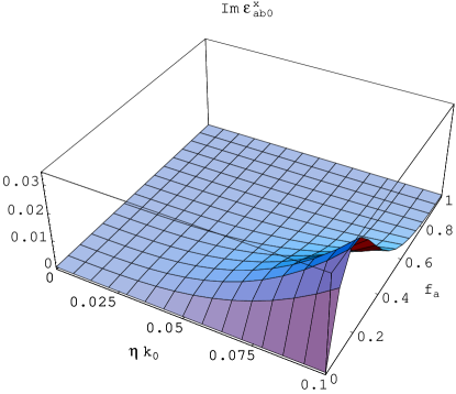
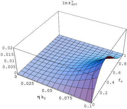
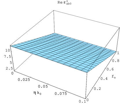
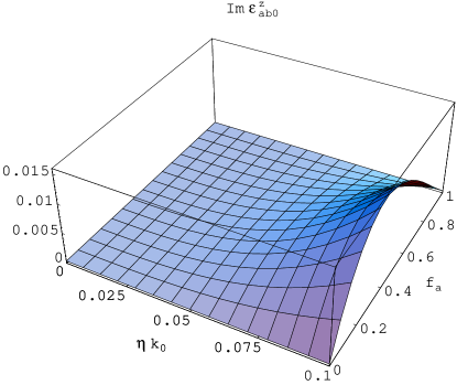
In Figure 1, the components of the zeroth order SPFT estimate of HCM permittivity $\underline{\underline{\epsilon}}^{[0]}_{\,ab}=\epsilon_{\scriptscriptstyle 0}\,\mbox{diag}\left(\epsilon^{x}_{ab0},\,\epsilon^{y}_{ab0},\,\epsilon^{z}_{ab0}\right)$ are plotted against volume fraction $f_{a}$ and relative inclusion size $k_{\scriptscriptstyle 0}\eta$. The permittivity parameters $\epsilon^{x,y,z}_{ab0}$ are constrained to agree with $\epsilon_{b}$ and $\epsilon_{a}$ at $f_{a}=0$ and $f_{a}=1$, respectively. For volume fractions $f_{a}\in(0,1)$, the ellipsoidal particulate geometry of the component phases endows the HCM with biaxial anisotropy and we observe that $\epsilon^{x}_{ab0}$, $\epsilon^{y}_{ab0}$, $\epsilon^{z}_{ab0}$, $\epsilon_{a}$ and $\epsilon_{b}$ each take different values. At $\eta=0$ the estimates of the HCM permittivity parameters $\epsilon^{x,y,z}_{ab0}$ are the same as those of the conventional Bruggeman homogenization formalism. When $\eta>0$ the parameters $\epsilon^{x,y,z}_{ab0}$ become complex-valued with positive imaginary parts, despite the component phase permittivities $\epsilon_{a}$ and $\epsilon_{b}$ being real-valued. The manifestation of $\mbox{Im}\,\left(\epsilon^{x,y,z}_{ab0}\right)>0$ indicates radiative scattering loss from the macroscopic coherent field [23]. Thus, we see that by attributing a nonzero volume to the component phase inclusions, coherent scattering is accommodated, thereby giving rise to a dissipative HCM. Since the imaginary parts of $\epsilon^{x,y,z}_{ab0}$ are observed to increase with increasing $\eta$, it is deduced that more radiation is scattered out of the coherent field by enlarging the depolarization volumes. The real parts of the HCM permittivity parameters $\epsilon^{x,y,z}_{ab0}$ are found to be relatively insensitive to the inclusion size parameter $\eta$.

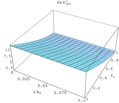
Let us turn now to the bilocally-approximated SPFT. For vanishingly small component phase inclusions (i.e., $\eta=0$), the components of the second order SPFT estimate of HCM permittivity $\underline{\underline{\epsilon}}^{[2]}_{\,ab}=\epsilon_{\scriptscriptstyle 0}\,\mbox{diag}\left(\epsilon^{x}_{ab2},\,\epsilon^{y}_{ab2},\,\epsilon^{z}_{ab2}\right)$ are graphed against volume fraction $f_{a}$ and relative correlation length $k_{\scriptscriptstyle 0}L$ in Figure 2. As $L\rightarrow 0$, the second order SPFT estimates converge to those of the zeroth order SPFT. Accordingly, the estimates of the HCM permittivity parameters $\epsilon^{x,y,z}_{ab2}$ at $L=0$ are the same as the estimates deriving from the conventional Bruggeman homogenization formalism. As the correlation length $L$ increases from 0, the HCM parameters $\epsilon^{x,y,z}_{ab2}$ acquire positive-valued imaginary parts. Furthermore, as $L$ increases so the imaginary parts of the HCM parameters $\epsilon^{x,y,z}_{ab2}$ become increasingly large. Thus, we infer that the scattering interactions of increasing numbers of component phase inclusions become correlated as $L$ increases, resulting in an increasingly dissipative HCM. The real parts of the HCM permittivity parameters $\epsilon^{x,y,z}_{ab2}$ do not vary significantly as the correlation length increases, as is illustrated in Figure 2. Notice that the relationship between the correlation length $L$ and the second order SPFT parameters $\epsilon^{x,y,z}_{ab2}$ for $\eta=0$ closely resembles the relationship between the inclusion size parameter $\eta$ and the zeroth order SPFT parameters $\epsilon^{x,y,z}_{ab0}$ presented in Figure 1.

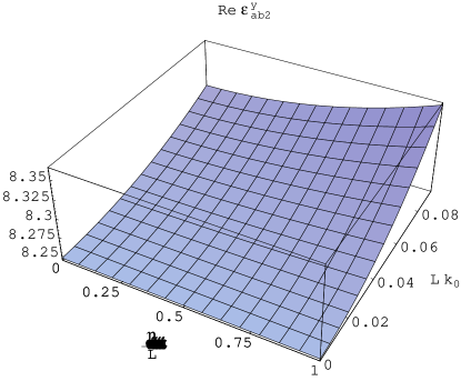
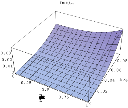
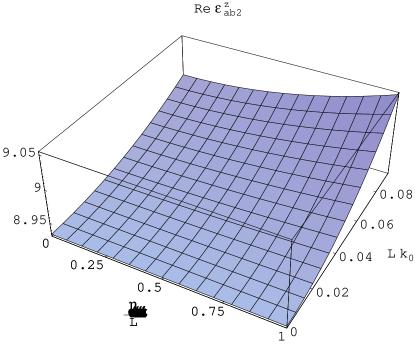
The result of combining an inclusion size parameter $\eta>0$ with a correlation length $L>0$ is presented in Figure 3. Therein, the components of the second order SPFT estimate $\underline{\underline{\epsilon}}^{[2]}_{\,ab}$ are plotted against both relative correlation length $k_{\scriptscriptstyle 0}L$ and the relative inclusion size $\eta/L$ for the fixed volume fraction $f_{a}=0.3$. The real and imaginary parts of the HCM permittivity parameters $\epsilon^{x,y,z}_{ab2}$ are seen to increase with both $\eta$ and $L$. Furthermore, the rate of increase of $\mbox{Im}\,\left(\epsilon^{x,y,z}_{ab2}\right)$ exceeds the corresponding rate of increase observed in Figure 1 when $L=0$, and in Figure 2 when $\eta=0$. Hence, by taking account of both nonzero depolarization volume and correlation length, more radiation is scattered out of the coherent field than would be the case if either nonzero depolarization volume or correlation length alone was taken into account.

4.2 Dissipative component phases

While it is instructive to consider nondissipative component phases in order to highlight the particular effects of depolarization volume and correlation length, in reality all mediums exhibit dissipation. Therefore, let us now consider the homogenization of component phases characterized by the complex-valued permittivities $\epsilon_{a}=\left(2+0.05i\right)\epsilon_{\scriptscriptstyle 0}$ and $\epsilon_{b}=\left(12+0.4i\right)\epsilon_{\scriptscriptstyle 0}$. We continue with the same values for the inclusion shape parameters $U_{x}$, $U_{y}$ and $U_{z}$ as given in (31). The volume fraction is fixed at $f_{a}=0.3$ for all results presented in this section.

In Figure 4, the components of the zeroth order SPFT estimate of HCM permittivity $\underline{\underline{\epsilon}}^{[0]}_{\,ab}$ are plotted against relative inclusion size $k_{\scriptscriptstyle 0}\eta$. Since the component phases are themselves dissipative, the imaginary parts of $\epsilon^{x,y,z}_{ab0}$ are positive-valued at $\eta=0$. As the inclusion size parameter $\eta$ increases, so the imaginary parts of $\epsilon^{x,y,z}_{ab0}$ also increase. The growth in $\mbox{Im}\,\left(\epsilon^{x,y,z}_{ab0}\right)$ is attributable to the increasing amount of coherent scattering loss which develops as the depolarization regions increase in size. As was observed in the corresponding instance for nondissipative component phases, the real parts of $\epsilon^{x,y,z}_{ab0}$ are relatively insensitive to $\eta$.

The second order SPFT estimates of the HCM permittivity parameters $\epsilon^{x,y,z}_{ab2}$, calculated with $\eta=0$, are graphed against relative correlation length $k_{\scriptscriptstyle 0}L$ in Figure 5. The observed increase in $\mbox{Im}\,\left(\epsilon^{x,y,z}_{ab0}\right)$ as $L$ increases reflects the fact that coherent losses increase as the actions of increasing numbers of scattering centres become correlated. The real parts of the HCM permittivity parameters vary little as the correlation length increases. Comparing Figures 4 and 5, it is clear that the dependency upon $L$ for the second-order SPFT with $\eta=0$ closely resembles the dependency upon $\eta$ for the zeroth order SPFT.

Finally, let us consider the combined effect of nonzero depolarization volume and correlation length. In Figure 6, $\epsilon^{x,y,z}_{ab2}$ are plotted against relative inclusion size $k_{\scriptscriptstyle 0}\eta$ for the fixed relative correlation length $k_{\scriptscriptstyle 0}L=0.1$. While $\mbox{Re}\,\left(\epsilon^{x,y,z}_{ab2}\right)$ are relatively insensitive to increasing $\eta$, $\mbox{Im}\,\left(\epsilon^{x,y,z}_{ab2}\right)$ increase markedly as the inclusion size parameter increases. Furthermore, the rate of increase of $\mbox{Im}\,\left(\epsilon^{x,y,z}_{ab2}\right)$ in Figure 6 is greater than that seen in Figure 4 where the influence of $\eta$ alone is considered, and in Figure 5 where the influence of $L$ alone is considered.

5 Concluding remarks

In implementations of homogenization formalisms, such as the widely-used Maxwell Garnett and Bruggeman formalisms, the distributional statistics and sizes of the component phase particles are often inadequately taken into account. A notable exception is provided by the SPFT in which the distributional statistics of the component phases are described through a hierarchy of spatial correlation functions. In the present study the SPFT is extended through attributing a nonzero volume to the component phase inclusions. Thereby, we show that both depolarization volume and correlation length contribute to coherent scattering losses. Furthermore, the effects of depolarization volume and correlation length upon the imaginary parts of the HCM constitutive parameters are cumulative and reflect the anisotropy of the HCM. We remark that our numerical results which relate to the effect of depolarization volume alone, as presented in presented in Figures 1 and 4, are consistent with numerical results based on the extended Maxwell Garnett and extended Bruggeman homogenization formalisms for isotropic dielectric HCMs [20, 32]. The importance of incorporating microstructural details within homogenization formalisms is thus further emphasized.

Acknowledgement: The author thanks an anonymous referee for suggesting improvements to the manuscript and drawing his attention to Ref. [23].

References

  • [1] Lakhtakia A (ed) 1996 Selected Papers on Linear Optical Composite Materials (Bellingham WA: SPIE Optical Engineering Press)
  • [2] Mackay TG 2003 Homogenization of linear and nonlinear complex composite materials Introduction to Complex Mediums for Optics and Electromagnetics ed WS Weiglhofer and A Lakhtakia (Bellingham WA: SPIE Press) pp 317–345
  • [3] Walser RM 2003 Metamaterials: an introduction Introduction to Complex Mediums for Optics and Electromagnetics ed WS Weiglhofer and A Lakhtakia (Bellingham, WA, USA: SPIE Press) pp 295–316
  • [4] Michel B 2000 Recent developments in the homogenization of linear bianisotropic composite materials Electromagnetic fields in unconventional materials and structures ed ON Singh and A Lakhtakia (New York: John Wiley and Sons) pp 39–82
  • [5] Faxén H 1920 Der Zusammenhang zwischen den Maxwellschen Gleichungen für Dielektrika und den atomistischen Ansätzen von H.A. Lorentz u.a. Zeitschrift für Physik 2, 218–229
  • [6] Lakhtakia A and Weiglhofer WS 1993 Maxwell-Garnett estimates of the effective properties of a general class of discrete random composites Acta Crystallographica A 49, 266–269
  • [7] Ryzhov Yu A and Tamoikin VV 1970 Radiation and propagation of electromagnetic waves in randomly inhomogeneous media Radiophys. Quantum Electron. 14 228–233
  • [8] Tsang L and Kong JA 1981 Scattering of electromagnetic waves from random media with strong permittivity fluctuations Radio Sci. 16 303–320
  • [9] Frisch U 1970 Wave propagation in random media Probabilistic Methods in Applied Mathematics Vol. 1 ed AT Bharucha–Reid (London: Academic Press) pp 75–198
  • [10] Zhuck NP and Lakhtakia A 1999 Effective constitutive properties of a disordered elastic solid medium via the strong–fluctuation approach Proc. R. Soc. Lond. A 455 543–566
  • [11] Genchev ZD 1992 Anisotropic and gyrotropic version of Polder and van Santen’s mixing formula Waves Random Media 2 99–110
  • [12] Zhuck NP 1994 Strong–fluctuation theory for a mean electromagnetic field in a statistically homogeneous random medium with arbitrary anisotropy of electrical and statistical properties Phys. Rev. B 50 15636–15645
  • [13] Michel B and Lakhtakia A 1995 Strong–property–fluctuation theory for homogenizing chiral particulate composites Phys. Rev. E 51 5701–5707
  • [14] Mackay TG, Lakhtakia A and Weiglhofer WS 2000 Strong–property–fluctuation theory for homogenization of bianisotropic composites: formulation Phys. Rev. E 62 6052–6064 Erratum 2001 63 049901
  • [15] Mackay TG and Lakhtakia A 2004 Correlation length facilitates Voigt wave propagation Waves Random Media 14 L1–L11
  • [16] Michel B 1997 A Fourier space approach to the pointwise singularity of an anisotropic dielectric medium Int. J. Appl. Electromagn. Mech. 8 219–227
  • [17] Michel B and Weiglhofer WS 1997 Pointwise singularity of dyadic Green function in a general bianisotropic medium Arch. Elekron. Übertrag. 51 219–223 Erratum 1998 52 31
  • [18] Doyle WT 1989 Optical properties of a suspension of metal spheres Phys. Rev. B 39 9852–9858
  • [19] Dungey CE and Bohren CF 1991 Light scattering by nonspherical particles: a refinement to the coupled-dipole method J. Opt. Soc. Am. A 8 81–87
  • [20] Prinkey MT, Lakhtakia A and Shanker B 1994 On the extended Maxwell–Garnett and the extended Bruggeman approaches for dielectric-in-dielectric composites Optik 96 25–30
  • [21] Shanker B and Lakhtakia A 1993 Extended Maxwell Garnett model for chiral–in–chiral composites J. Phys. D: Appl. Phys. 26 1746–1758
  • [22] Shanker B 1996 The extended Bruggeman approach for chiral–in–chiral mixtures J. Phys. D: Appl. Phys. 29 281–288
  • [23] Van Kranendonk J and Sipe JE 1977 Foundations of the macroscopic electromagnetic theory of dielectric media Progress in Optics XV ed E Wolf (Amsterdam: North–Holland) pp 245–350
  • [24] Weiglhofer WS 1993 Analytic methods and free–space dyadic Green’s functions Radio Sci. 28 847–857
  • [25] Weiglhofer WS 1998 Electromagnetic depolarization dyadics and elliptic integrals J. Phys. A: Math. Gen. 31 7191–7196
  • [26] Bohren CF and Huffman DR 1983 Absorption and Scattering of Light by Small Particles (New York: Wiley)
  • [27] Mackay TG 2003 Geometrically derived anisotropy in cubically nonlinear dielectric composites J. Phys. D: Appl. Phys. 36 583–591
  • [28] Press WH, Flannery BP, Teukolsky SA and Vetterling WT 1992 Numerical Recipes in Fortran 2nd Edition (Cambridge: Cambridge University Press)
  • [29] Tsang L, Kong JA and Newton RW 1982 Application of strong fluctuation random medium theory to scattering of electromagnetic waves from a half–space of dielectric mixture IEEE Trans. Antennas Propagat. 30 292–302
  • [30] Mackay TG, Lakhtakia A and Weiglhofer WS 2001 Homogenisation of similarly oriented, metallic, ellipsoidal inclusions using the bilocally approximated strong–property–fluctuation theory Opt. Commun. 107 89–95
  • [31] Mackay TG and Lakhtakia A 2004 A limitation of the Bruggeman formalism for homogenization Opt. Commun. 234 35–42
  • [32] Shanker B and Lakhtakia A 1993 Extended Maxwell Garnett formalism for composite adhesives for microwave-assisted adhesion of polymer surfaces J. Composite Mater. 27 1203–1213
Refer to caption
Refer to caption
Refer to caption
Refer to caption
Refer to caption
Refer to caption
Figure 1: Real (left) and imaginary (right) parts of the zeroth order SPFT estimate of HCM permittivity $\,\underline{\underline{\epsilon}}^{[0]}_{\,ab}=\epsilon_{\scriptscriptstyle 0}\,\mbox{diag}\left(\epsilon^{x}_{ab0},\,\epsilon^{y}_{ab0},\,\epsilon^{z}_{ab0}\right)$ plotted against volume fraction $f_{a}$ and relative inclusion size $k_{\scriptscriptstyle 0}\eta$. Component phase parameter values: $\epsilon_{a}=2\epsilon_{\scriptscriptstyle 0}$, $\epsilon_{b}=12\epsilon_{\scriptscriptstyle 0}$, $U_{x}=1$, $U_{y}=3$ and $U_{z}=15$.
Refer to caption
Refer to caption
Refer to caption
Refer to caption
Refer to caption
Refer to caption
Figure 2: Real (left) and imaginary (right) parts of the second order SPFT estimate of HCM permittivity $\,\underline{\underline{\epsilon}}^{[2]}_{\,ab}=\epsilon_{\scriptscriptstyle 0}\,\mbox{diag}\left(\epsilon^{x}_{ab2},\,\epsilon^{y}_{ab2},\,\epsilon^{z}_{ab2}\right)$ plotted against volume fraction $f_{a}$ and relative correlation length $k_{\scriptscriptstyle 0}L$, with inclusion size parameter $\eta=0$. Component phase permittivities $\epsilon_{a}$ and $\epsilon_{b}$, and shape parameters $U_{x}$, $U_{y}$ and $U_{z}$, as in Figure 1.
Refer to caption
Refer to caption
Refer to caption
Refer to caption
Refer to caption
Refer to caption
Figure 3: Real (left) and imaginary (right) parts of the second order SPFT estimate of HCM permittivity $\,\underline{\underline{\epsilon}}^{[2]}_{\,ab}=\epsilon_{\scriptscriptstyle 0}\,\mbox{diag}\left(\epsilon^{x}_{ab2},\,\epsilon^{y}_{ab2},\,\epsilon^{z}_{ab2}\right)$ plotted relative correlation length $k_{\scriptscriptstyle 0}L$ and relative inclusion size parameter $\eta/L$, with volume fraction $f_{a}=0.3$. Component phase permittivities $\epsilon_{a}$ and $\epsilon_{b}$, and shape parameters $U_{x}$, $U_{y}$ and $U_{z}$, as in Figure 1.
Refer to caption
Refer to caption
Figure 4: Real (top) and imaginary (bottom) parts of the zeroth order SPFT estimate of HCM permittivity $\,\underline{\underline{\epsilon}}^{[0]}_{\,ab}=\epsilon_{\scriptscriptstyle 0}\,\mbox{diag}\left(\epsilon^{x}_{ab0},\,\epsilon^{y}_{ab0},\,\epsilon^{z}_{ab0}\right)$ plotted against relative inclusion size $k_{\scriptscriptstyle 0}\eta$ for volume fraction $f_{a}=0.3$. Component phase parameter values: $\epsilon_{a}=\left(2+0.05i\right)\epsilon_{\scriptscriptstyle 0}$, $\epsilon_{b}=\left(12+0.4i\right)\epsilon_{\scriptscriptstyle 0}$, $U_{x}=1$, $U_{y}=3$ and $U_{z}=15$. Key: $\epsilon^{x}_{ab0}$, $\epsilon^{y}_{ab0}$ and $\epsilon^{z}_{ab0}$ are denoted by solid, broken dashed and dashed lines respectively.
Refer to caption
Refer to caption
Figure 5: Real (top) and imaginary (bottom) parts of the second order SPFT estimate of HCM permittivity $\,\underline{\underline{\epsilon}}^{[2]}_{\,ab}=\epsilon_{\scriptscriptstyle 0}\,\mbox{diag}\left(\epsilon^{x}_{ab2},\,\epsilon^{y}_{ab2},\,\epsilon^{z}_{ab2}\right)$ plotted against relative correlation length $k_{\scriptscriptstyle 0}L$, with inclusion size parameter $\eta=0$ and volume fraction $f_{a}=0.3$. Component phase permittivities $\epsilon_{a}$ and $\epsilon_{b}$, and shape parameters $U_{x}$, $U_{y}$ and $U_{z}$, as in Figure 4. Key: $\epsilon^{x}_{ab2}$, $\epsilon^{y}_{ab2}$ and $\epsilon^{z}_{ab2}$ are denoted by solid, broken dashed and dashed lines respectively.
Refer to caption
Refer to caption
Figure 6: Real (top) and imaginary (bottom) parts of the second order SPFT estimate of HCM permittivity $\,\underline{\underline{\epsilon}}^{[2]}_{\,ab}=\epsilon_{\scriptscriptstyle 0}\,\mbox{diag}\left(\epsilon^{x}_{ab2},\,\epsilon^{y}_{ab2},\,\epsilon^{z}_{ab2}\right)$ plotted relative inclusion size parameter $k_{\scriptscriptstyle 0}\eta$, with relative correlation length $k_{\scriptscriptstyle 0}L=0.1$ and volume fraction $f_{a}=0.3$. Component phase permittivities $\epsilon_{a}$ and $\epsilon_{b}$, and shape parameters $U_{x}$, $U_{y}$ and $U_{z}$, as in Figure 4; and key as in Figure 5.