Thermodynamics of MHD flows with axial symmetry

Abstract

We present strategies based upon extremization principles, in the case of the axisymmetric equations of magnetohydrodynamics (MHD). We study the equilibrium shape by using a minimum energy principle under the constraints of the MHD axisymmetric equations. We also propose a numerical algorithm based on a maximum energy dissipation principle to compute in a consistent way the equilibrium states. Then, we develop the statistical mechanics of such flows and recover the same equilibrium states giving a justification of the minimum energy principle. We find that fluctuations obey a Gaussian shape and we make the link between the conservation of the Casimirs on the coarse-grained scale and the process of energy dissipation.

I Introduction

The recent success of two experimental fluid dynamos Gailitis01 ; Stieglitz01 has renewed the interest in the mechanism of dynamo saturation, and, thus, of equilibrium configurations in MHD. At the present time, there is no general theory to tackle this problem, besides dimensional theory. For example, in a conducting fluid with typical velocity $V$, density $\rho$ , Reynolds number $Re$ and magnetic Prandtl number $Pm$, the typical level of magnetic field reached at saturation is necessarily Petrelis01 :

$$B^{2}=\mu_{o}\rho V^{2}f(Re,Pm),$$ (1)

where $f$ is a priori an arbitrary function of $Re$ and $Pm$. Many numerical simulations Archontis00 lead to $f=1$, i.e. equipartition between the magnetic and turbulent energy. This is therefore often taken as a working tool in astrophysical or geophysical application. However, this result is far from applying to any saturated dynamo. Moreover, it does not give any information about possible anisotropy of the saturated field. It would therefore be interesting to build robust algorithms to derive the function $f$. By robust, we mean algorithm which depends on characteristic global quantities of the system (like total energy) but not necessarily on small-scale dissipation, or boundary conditions.

An interesting candidate in this regards is provided by statistical mechanics. In the case of pure fluid mechanics, statistical mechanics has mainly been developed within the frame of Euler equation for a two-dimensional perfect fluid. Onsager Onsager49 first used a Hamiltonian model of point vortices. Within this framework, turbulence is a state of negative temperature leading to the coalescence of vortices of same sign Montgomery74 . Further improvement were provided by Miller et al. Miller90 and Robert and Sommeria Robert91 who independently introduced a discretization of the vorticity in a certain number of levels to account for the continuous nature of vorticity. Using the maximum entropy formalism of statistical mechanics Jaynes57 , it is then possible to give the shape of the (meta)-equilibrium solution of Euler’s equation as well as the fine-grained fluctuations around it jfm1 . This is similar to Lynden-Bell’s theory of violent relaxation lb in stellar dynamics (see Chavanis houches for a description of the analogy between 2D vortices and stellar systems). The predictive power of the statistical theory is however limited by the existence of an infinite number of constants (the Casimirs) which precludes the finding of an universal Gibbs state. In particular, the metaequilibrium state strongly depends on the details of the initial condition. In certain occasions, for instance when the flow is forced at small scales, it may be more relevant to fix a prior distribution of vorticity fluctuations instead of the Casimirs ellis . Then, the coarse-grained flow maximizes a “generalized” entropy functional determined by the prior distribution of vorticity Chavanis03 . The statistical mechanics of MHD flows has been recently explored by Jordan and Turkington Jordan97 in 2D. In contrast with non-magnetized 2D hydrodynamics they obtained a universal Gaussian shape for the fluctuations. This comes from the fact that the conserved quantity in the MHD case is an integral quantity of the primitive velocity and magnetic fields and thus, in the continuum limit, has vanishing fluctuations.

The pure 2D situation however seldom applies to astrophysical or geophysical flows. In this respect, it is interesting to develop statistical mechanics of systems closer to natural situations, albeit sufficiently simple so that the already well tested recipes of statistical mechanics apply. These requirements are met by flows with axial symmetry. Most natural objects are rotating, selecting this peculiar symmetry. Moreover, upon shifting from 2D to axi-symmetric flows, one mainly shifts from a translation invariance along one axis, towards a rotation invariance along one axis. Apart from important physical consequences which need to be taken into account (for example conservation of angular momentum instead of vorticity or momentum, curvature terms), this induces a similarity between the two systems which enables a natural adaptation of the 2D case to the axisymmetric case. This is shown in the present paper, where we recover the Gaussian shape of the fluctuations and make the link between the conservation of the Casimirs on the coarse-grained scale and the process of energy dissipation.

In the first part of the paper, we study the equilibrium shape by using a minimum energy principle under the constraints of the MHD axisymmetric equations. We also propose a numerical algorithm based on a maximum energy dissipation principle to compute in a consistent way the equilibrium states. This is similar to the relaxation equation proposed by Chavanis Chavanis03 in 2D hydrodynamics to construct stable stationary solutions of the Euler equation by maximizing the production of a $H$-function. Then, we develop the statistical mechanics of such flows and recover these equilibrium states, thereby providing a physical justification for the minimum energy principle.

II MHD flows with axial symmetry

II.1 Equations and notations

Consider the ideal incompressible MHD equations:

$$\partial_{t}{\bf U}+({\bf U}\cdot\nabla){\bf U} = -\frac{1}{\rho}\nabla P+({\bf\nabla}\times{\bf B})\times{\bf B}\,,$$

$$\partial_{t}{\bf B}+({\bf U}\cdot\nabla){\bf B} = ({\bf B}\cdot\nabla){\bf U}\,,$$ (2)

where ${\bf U}$ is the fluid velocity, $P$ is the pressure, $\sqrt{\rho\mu_{0}}\,{\bf B}$ is the magnetic field and $\rho$ is the (constant) fluid density. In the axisymmetric case we consider, it is convenient to introduce the poloidal/toroidal decomposition for the fields ${\bf U}$ and ${\bf B}$:

$${\bf U} = {\bf U_{p}}+{\bf U_{t}}={\bf U_{p}}+U\,{\bf e_{\theta}}\,,$$ (3)

$${\bf B} = {\bf B_{p}}+{\bf B_{t}}={\bf\nabla}\times(A{\bf e_{\theta}})+B\,{\bf e_{\theta}}\,,$$

where ${\bf A}={\bf A_{p}}+A\,{\bf e_{\theta}}$ is the potential vector. This decomposition will be used in our statistical mechanics approach.

When considering energy methods, we shall introduce alternate fields, built upon the poloidal and toroidal decomposition. They are : $\sigma_{u}=rU$, $\sigma_{b}=rA$, $\xi_{u}=\omega/r$ and $\xi_{b}=B/r$, where $\omega$ is the toroidal part of the vorticity field. In these variables, the ideal incompressible MHD equations (2) become, in the axisymmetric approximation, a set of four scalar equations:

$$\partial_{t}\sigma_{b}+\{\psi,\sigma_{b}\} = 0\,,$$ (4)

$$\partial_{t}\xi_{b}+\{\psi,\xi_{b}\} = \{\sigma_{b},\frac{\sigma_{u}}{2y}\}\,,$$

$$\partial_{t}\sigma_{u}+\{\psi,\sigma_{u}\} = \{\sigma_{b},2y\xi_{b}\}\,,$$

$$\partial_{t}\xi_{u}+\{\psi,\xi_{u}\} = \partial_{z}(\frac{\sigma_{u}^{2}}{4y^{2}}-\xi_{b}^{2})-\{\sigma_{b},\Delta_{*}\sigma_{b}\}\,,$$

where the fields are function of the axial coordinate $z$ and the modified radial coordinate $y=r^{2}/2$ and $\psi$ is a stream function: ${\bf U_{p}}={\bf\nabla}\times(\psi/r\quad{\bf e_{\theta}})$. We have introduced a Poisson Bracket: $\{f,g\}=\partial_{y}f\partial_{z}g-\partial_{z}f\partial_{y}g$. We also defined a pseudo Laplacian in the new coordinates:

$$\Delta_{*}=\frac{\partial^{2}}{\partial y^{2}}+\frac{1}{2y}\frac{\partial^{2}}{\partial z^{2}}\,.$$ (5)

Following Jordan97 , we will make an intensive use of the operators (for more details, see appendix A): $curl$ which gives the toroidal part of the curl of any vector and ${\bf Curl}$ which takes a toroidal field as argument and returns the poloidal part of the curl. If $j=curl{\bf B}$ is the toroidal part of the current and $\psi=r\,Curl^{-1}({\bf U_{p}})$, the following relations hold:

$$\xi_{u} = -\Delta_{*}\psi\,,$$ (6)

$$j/r = -\Delta_{*}\sigma_{b}\,.$$ (7)

Under the shape (4), the ideal axisymmetric MHD equation of motion lead to the immediate identification of $\sigma_{b}=rA$ as a conserved quantity associated to axial symmetry. This quantity is only advected by the velocity field and thus should play a special role regarding the global conserved quantities, as we now show.

II.2 Conservation laws

II.2.1 General case

The whole set of conservation laws of the axisymmetric ideal MHD equations have been derived by Woltjer Woltjer59 :

$$I = \int C(\sigma_{b})\,dydz\,,$$ (8)

$$H_{m} = 2\int\xi_{b}N(\sigma_{b})\,dydz\,,$$

$$H_{c} = \int\{F(\sigma_{b})\xi_{u}+\sigma_{u}\xi_{b}F^{\prime}(\sigma_{b})\}\,dydz\,,$$

$$L = \int\sigma_{u}G(\sigma_{b})\,dydz\,,$$

$$E = \frac{1}{2}\int\biggl{\{}\xi_{u}\psi-\sigma_{b}\Delta_{*}\sigma_{b}+\frac{\sigma_{u}^{2}}{2y}+2y\xi_{b}^{2}\biggr{\}}\,dydz\,.$$

where $C$, $N$, $F$ and $G$ are arbitrary functions. One can check that these integrals are indeed constants of motion by using (4) and the following boundary conditions: $\sigma_{b}=\sigma_{u}=\xi_{u}=\xi_{b}=0$ on the frontier of the domain. To prove the constancy of the third integral, one has to suppose that $F(0)=0$. The interpretation of these integrals of motion is easier when considering a special case, introduced by Chandrasekhar Chandrasekhar58 .

II.2.2 Chandrasekhar model

The conservation laws take a simpler shape when one considers only linear and quadratic conservation laws, such that Chandrasekhar58 $N(\sigma_{b})=F(\sigma_{b})=G(\sigma_{b})=\sigma_{b}$ and $N(\sigma_{b})=G(\sigma_{b})=1$ . The case $F(\sigma_{b})=1$ is forbidden by the condition that $F$ should vanish at the origin. In that case, the set of conserved quantities can be split in two families. The first one is made-up with conserved quantities of the ideal MHD system, irrespectively of the geometry:

$$H_{m} = 2\int\xi_{b}\sigma_{b}\,dydz=\int{\bf A}\cdot{\bf B}\,d{\bf x}=2\int AB\,d{\bf x}\,,$$ (9)

$$H_{c} = \int\{\sigma_{b}\xi_{u}+\sigma_{u}\xi_{b}\}\,dydz=\int{\bf U}\cdot{\bf B}\,d{\bf x}\,,$$

$$E = \frac{1}{2}\int\biggl{\{}\xi_{u}\psi-\sigma_{b}\Delta_{*}\sigma_{b}+\frac{\sigma_{u}^{2}}{2y}+2y\xi_{b}^{2}\biggr{\}}\,dydz=\frac{1}{2}\int({\bf U}^{2}+{\bf B}^{2})\,d{\bf x}\,,$$

where $H_{m}$ is the magnetic helicity, $H_{c}$ is the cross-helicity and $E$ is the total energy. Note that due to the Lorentz force, the kinetic helicity is not conserved, unlike in the pure hydrodynamical case. The other family of conserved quantities is made of the particular integrals of motion which appear due to axisymmetry:

$$I = \int C(\sigma_{b})dydz=\int C(rA)\,d{\bf x}\,,$$ (10)

$$H_{m}^{\prime} = 2\int\xi_{b}\,dydz=\int\frac{B}{r}d{\bf x}\,,$$

$$L = \int\sigma_{u}G(\sigma_{b})\,dydz=\int r^{2}UB\,d{\bf x}\,,$$

$$L^{\prime} = \int\sigma_{u}\,dydz=\int rU\,d{\bf x}\,.$$

Apart from $L^{\prime}$ the angular momentum, it is difficult to give the other quantities any physical interpretation. The class of invariant $I$ are called the Casimirs of the system (if one defines a non canonical bracket for the Hamiltonian system, they commute, in the bracket sense, will all other functionals). The conservation laws found by Woltjer are then generalization of these quantities.

II.3 Dynamical stability

II.3.1 General case

Following Woltjer59 , we show that the extremization of energy at fixed $I$, $H_{m}$, $H_{c}$ and $L$ determines the general form of stationary solutions of the MHD equations. We argue that the solutions that minimize the energy are nonlinearly dynamically stable for the inviscid equations.

To make the minimization, we first note that each integral is equivalent to an infinite set of constraints. Following Woltjer, we shall introduce a complete set of functions and label these functions and the corresponding integrals with an index $n$. Then, introducing Lagrange multipliers for each constraint, to first order, the variational problem takes the form:

$$\delta E+\sum_{n=1}^{+\infty}\biggl{\{}\alpha^{(n)}\delta I^{(n)}+\mu_{m}^{(n)}\delta H_{m}^{(n)}+\mu_{c}^{(n)}\delta H_{c}^{(n)}+\gamma^{(n)}\delta L^{(n)}\biggr{\}}=0\,.$$ (11)

Taking the variations on $\sigma_{b}$, $\xi_{b}$, $\sigma_{u}$ and $\xi_{u}$, we find:

$$\Delta_{*}\sigma_{b} = -F^{\prime}(\sigma_{b})\Delta_{*}\psi+F^{\prime\prime}(\sigma_{b})\sigma_{u}\xi_{b}+G^{\prime}(\sigma_{b})\sigma_{u}+2N^{\prime}(\sigma_{b})\xi_{b}+C^{\prime}(\sigma_{b})\,,$$ (12)

$$2y\xi_{b} = -2N(\sigma_{b})-F^{\prime}(\sigma_{b})\sigma_{u}\,,$$

$$\frac{\sigma_{u}}{2y} = -F^{\prime}(\sigma_{b})\xi_{b}-G(\sigma_{b})\,,$$

$$\psi = -F(\sigma_{b})\,,$$

where we have set $F(\sigma_{b})=\sum_{n=0}^{+\infty}\mu_{c}^{(n)}F_{n}(\sigma_{b})$ and similar notations for the other functions. This is the general solution of the incompressible axisymmetric ideal MHD problem Woltjer59 . In the general case, it is possible to express the three field $\sigma_{u}$, $\xi_{u}$ and $\xi_{b}$ in terms of $\sigma_{b}$. Then the first equation of the above system leads a partial differential equation for $\sigma_{b}$ to be solved to find the equilibrium distribution. Note that the extremization of the “free energy” $J=E+\alpha I+\mu_{m}H_{m}+\mu_{c}H_{c}+\gamma L$ yields the same equations as (12). Differences will appear on the second order variations (see below).

II.3.2 Chandrasekhar model

In the Chandrasekhar model, the arbitrary functions are at most linear functions of $\sigma_{b}$: $N(\sigma_{b})=\mu_{m}\sigma_{b}+\mu^{\prime}_{m}$, $F(\sigma_{b})=\mu_{c}\sigma_{b}$ and $G(\sigma_{b})=\gamma\sigma_{b}+\gamma^{\prime}$. Thus the stationary profile in the Chandrasekhar model is given by:

$$\Delta_{*}\sigma_{b} = -\mu_{c}\Delta_{*}\psi+\gamma\sigma_{u}+2\mu_{m}\xi_{b}+C^{\prime}(\sigma_{b})\,,$$ (13)

$$2y\xi_{b} = -2\mu_{m}\sigma_{b}-2\mu^{\prime}_{m}-\mu_{c}\sigma_{u}\,,$$

$$\frac{\sigma_{u}}{2y} = -\mu_{c}\xi_{b}-\gamma\sigma_{b}-\gamma^{\prime}\,,$$

$$\psi = -\mu_{c}\sigma_{b}\,.$$

From the previous equations, we obtain

$$2y(1-\mu_{c}^{2})\xi_{b} = 2(\gamma\mu_{c}y-\mu_{m})\sigma_{b}+2\mu_{c}\gamma^{\prime}y-2\mu^{\prime}_{m}\,,$$ (14)

$$(1-\mu_{c}^{2})\sigma_{u} = 2(\mu_{c}\mu_{m}-\gamma y)\sigma_{b}+2\mu_{c}\mu^{\prime}_{m}-2\gamma^{\prime}y\,,$$

$$\psi = -\mu_{c}\sigma_{b}\,,$$

where $\sigma_{b}$ is given by the differential equation:

$$(1-\mu_{c}^{2})^{2}\Delta_{*}\sigma_{b}=\Phi(\sigma_{b})-[2\mu_{m}^{2}\frac{\sigma_{b}}{y}+2\gamma^{2}y]\sigma_{b}-2\gamma\gamma^{\prime}y-\frac{2\mu_{m}\mu^{\prime}_{m}}{y}\,.$$ (15)

These expressions can be used to prove that these fields are stationary solutions of the axisymmetric MHD equations. We now turn to the stability problem. Since the free energy $J=E+\alpha I+\mu_{m}H_{m}+\mu_{c}H_{c}+\gamma L$ is conserved by the ideal dynamics, a minimum of $J$ will be nonlinearly dynamically stable (at least in the formal sense of Holm et al. Holm85 ). Note that this implication is not trivial because the system under study is dimensionally infinite. We will admit that their analysis can be generalized to the axisymmetric case. Since the integrals which appear in the free energy are conserved individually, a minimum of energy at fixed other constraints also determines a nonlinearly dynamically stable stationary solution of the MHD equations. This second stability criterion is stronger than the first (it includes it). We shall not prove these results, nor write the second order variations, here.

II.4 Numerical algorithm

II.4.1 General case

It is usually difficult to solve directly the system of equations (14)-(15) and make sure that they yield a stable stationary solution of the MHD equations. Instead, we shall propose a set of relaxation equations which minimize the energy while conserving any other integral of motion. This permits to construct solutions of the system (14)-(15) which are energy minima and respect the other constraints. A physical justification of this precedure linked to the dissipation of energy will be given in Sec. III.3.1.

Our relaxation equations can be written under the generic form

$$\frac{\partial\sigma}{\partial t}=-\nabla\cdot{\bf J}_{\sigma},$$ (16)

where $\sigma$ stands for $\sigma_{b}$, $\xi_{b}$, $\sigma_{u}$ or $\xi_{u}$. Using straightforward integration by parts, we then get:

$$\dot{I} = \int{\bf J}_{\sigma_{b}}\cdot[\nabla C^{\prime}(\sigma_{b})]dydz\,,$$ (17)

$$\dot{H}_{m} = 2\int\biggl{\{}{\bf J}_{\xi_{b}}\cdot\nabla[N(\sigma_{b})]+{\bf J}_{\sigma_{b}}\cdot\nabla[N^{\prime}(\sigma_{b})\xi_{b}]\biggr{\}}dydz\,,$$

$$\dot{H}_{c} = \int\biggl{\{}{\bf J}_{\xi_{u}}\cdot\nabla[F(\sigma_{b})]+{\bf J}_{\sigma_{b}}\cdot\nabla[F^{\prime}(\sigma_{b})\xi_{u}+F^{\prime\prime}(\sigma_{b})\sigma_{u}\xi_{b}]$$

$$+ {\bf J}_{\sigma_{u}}\cdot\nabla[F^{\prime}(\sigma_{b})\xi_{b}]+{\bf J}_{\xi_{b}}\cdot\nabla[F^{\prime}(\sigma_{b})\sigma_{u}]\biggr{\}}dydz\,,$$

$$\dot{L} = \int\biggl{\{}{\bf J}_{\sigma_{u}}\cdot\nabla[G(\sigma_{b})]+{\bf J}_{\sigma_{b}}\cdot\nabla[G^{\prime}(\sigma_{b})\sigma_{u}]\biggr{\}}dydz\,,$$

$$\dot{E} = \int\biggl{\{}{\bf J}_{\xi_{u}}\cdot\nabla\psi-{\bf J}_{\sigma_{b}}\cdot\nabla(\Delta_{*}\sigma_{b})+{\bf J}_{\sigma_{u}}\cdot\nabla\biggl{(}\frac{\sigma_{u}}{2y}\biggr{)}+{\bf J}_{\xi_{b}}\cdot\nabla(2y\xi_{b})\biggr{\}}dydz\,.$$

To construct the optimal currents, we rely on a procedure of maximization of the rate of dissipation of energy $\dot{E}$ very similar to the procedure of maximum entropy production principle (MEPP) of Robert and Sommeria Robert92 in the 2D turbulence case. This is equivalent to say that the evolution towards the equilibrium state (14)-(15) is very rapid. We thus try to maximize $\dot{E}$ given the conservation of $\dot{I}$, $\dot{H}_{m}$, $\dot{H}_{c}$ and $\dot{L}$. Such maximization can only have solution for bounded currents (if not, the fastest evolution is for infinite currents). Therefore, we also impose a bound on $J_{\sigma}^{2}$ where, as before, $\sigma$ stands for $\sigma_{b}$, $\xi_{b}$, $\sigma_{u}$, $\xi_{u}$.

Writing the variational problem under the form

$$\delta\dot{E}+\sum_{n=1}^{+\infty}\biggl{\{}\alpha^{(n)}(t)\delta\dot{I}^{(n)}+\mu_{m}^{(n)}(t)\delta\dot{H}_{m}^{(n)}+\mu_{c}^{(n)}(t)\delta\dot{H}_{c}^{(n)}+\gamma^{(n)}(t)\delta\dot{L}^{(n)}\biggr{\}}-\sum_{\sigma}\frac{1}{D_{\sigma}}\delta\biggl{(}\frac{J_{\sigma}^{2}}{2}\biggr{)}=0$$ (18)

and taking variations on ${\bf J}_{\sigma_{b}}$, ${\bf J}_{\xi_{b}}$, ${\bf J}_{\sigma_{u}}$, ${\bf J}_{\xi_{u}}$, we obtain the optimal currents. Inserting their expressions in the relaxation equations (16), we get:

$$\frac{\partial\sigma_{b}}{\partial t} = \nabla\cdot\biggl{\{}D_{\sigma_{b}}\nabla\cdot\biggl{[}-\Delta_{*}\sigma_{b}+C^{\prime}(\sigma_{b},t)+2\xi_{b}N^{\prime}(\sigma_{b},t)$$

$$+ \xi_{u}F^{\prime}(\sigma_{b},t)+\sigma_{u}\xi_{b}F^{\prime\prime}(\sigma_{b},t)+G^{\prime}(\sigma_{b},t)\sigma_{u}\biggr{]}\biggr{\}}\,,$$

$$\frac{\partial\xi_{b}}{\partial t} = \nabla\cdot\biggl{\{}D_{\xi_{b}}\nabla\cdot\biggl{[}2y\xi_{b}+2N(\sigma_{b},t)+F^{\prime}(\sigma_{b},t)\sigma_{u}\biggr{]}\biggr{\}}\,,$$

$$\frac{\partial\sigma_{u}}{\partial t} = \nabla\cdot\biggl{\{}D_{\sigma_{u}}\nabla\cdot\biggl{[}\frac{\sigma_{u}}{2y}+\xi_{b}F^{\prime}(\sigma_{b},t)+G(\sigma_{b},t)\biggr{]}\biggr{\}}\,,$$

$$\frac{\partial\xi_{u}}{\partial t} = \nabla\cdot\biggl{\{}D_{\xi_{u}}\nabla\cdot[\psi+F(\sigma_{b},t)]\biggr{\}}.$$

where we have set $F(\sigma_{b},t)=\sum_{n=0}^{+\infty}\mu_{c}^{(n)}(t)F_{n}(\sigma_{b})$ and similar notations for the other functions. The time evolution of the Lagrange multipliers $\mu_{c}^{(n)}(t)$ etc. are obtained by substituting the optimal currents in the constraints $\dot{H}_{c}^{(n)}=0$ etc. and solving the resulting set of algebraic equations. Using the expression of the optimal currents and the condition that $\dot{I}=\dot{H}_{m}=\dot{H}_{c}=\dot{L}=0$, we can show that:

$$\dot{E}=-\int\biggl{\{}\frac{J_{\xi_{u}}^{2}}{D_{\xi_{u}}}+\frac{J_{\sigma_{b}}^{2}}{D_{\sigma_{b}}}+\frac{J_{\sigma_{u}}^{2}}{D_{\sigma_{u}}}+\frac{J_{\xi_{b}}^{2}}{D_{\xi_{b}}}\biggr{\}}dydz\leq 0,$$ (20)

provided that the diffusion currents $D_{\xi_{u}}$, $D_{\sigma_{b}}$,$D_{\sigma_{u}}$ and $D_{\xi_{b}}$ are positive. Thus, the energy decreases until all the currents vanish. In that case, we obtain the static equations (12). In addition, this numerical algorithm guarantees that only energy minima (not maxima or saddle points) are reached. Note that if we fix the Lagrange multipliers instead of the constraints, the foregoing relaxation equations lead to a stationary state which minimizes the free energy $J$. Then, as stated above, the constructed solutions will be nonlinearly dynamical stable solution of the MHD set of equations. However, not allowing the Lagrange multiplier to depend on time, we may ”miss” some stable solutions of the problem. Indeed, we know that minima of the free energy are nonlinearly stable solutions of the problem but we do not know if they are the only ones: some solutions can be minima of $E$ at fixed $I$, $H_{m}$, $H_{c}$ and $L$ while they are not minima of $J=E+\alpha I+\mu_{m}H_{m}+\mu_{c}H_{c}+\gamma L$.

II.4.2 Chandrasekhar model

In the Chandrasekhar model (with $\mu^{\prime}_{m}=\gamma^{\prime}=0$), the previous equations can be simplified. The equilibrium solution does not depend on the particular value of the diffusion coefficients (these are only multiplicative factors of the optimal currents) and for simplicity, we set $D_{\xi_{u}}=D_{\sigma_{b}}=D_{\sigma_{u}}=D_{\xi_{b}}=1$. The relaxation equations then reduce to:

$$\frac{\partial\sigma_{b}}{\partial t} = \Delta\biggl{\{}-\Delta_{*}\sigma_{b}+C^{\prime}(\sigma_{b},t)+2\mu_{m}(t)\xi_{b}+\mu_{c}(t)\xi_{u}+\gamma(t)\sigma_{u}\biggr{\}}\,,$$ (21)

$$\frac{\partial\xi_{b}}{\partial t} = \Delta\biggl{\{}2y\xi_{b}+2\mu_{m}(t)\sigma_{b}+\mu_{c}(t)\sigma_{u}\biggr{\}}\,,$$

$$\frac{\partial\sigma_{u}}{\partial t} = \Delta\biggl{\{}\frac{\sigma_{u}}{2y}+\mu_{c}(t)\xi_{b}+\gamma(t)\sigma_{b}\biggr{\}}\,,$$

$$\frac{\partial\xi_{u}}{\partial t} = \Delta\{\psi+\mu_{c}(t)\sigma_{b}\}.$$

where the Lagrange multipliers evolve in time so as to conserve the constraints (17).

These equations are the MHD counterpart of the relaxation equations proposed by Chavanis Chavanis03 for 2D hydrodynamical flows described by the Euler equation. In this context, a stable stationary solution of the Euler equation maximizes a H-function (playing the role of a generalized entropy) at fixed energy and circulation. A justification of this procedure, linked to the increase of H-functions on the coarse-grained scale, will be further discussed in Sec. IV and compared with the MHD case.

If we set the velocity field to zero ($\sigma_{u}=\xi_{u}=0$), we get a system of equations linking the poloidal part ($\sigma_{b}$) and the toroidal part ($\xi_{b}$) of the magnetic field. It is fairly easy to see that the coupling between the two quantities is proportional to $\mu_{m}$ the Lagrange multiplier associated to the conservation of magnetic helicity. This is reminiscent of the $\alpha$ effect of dynamo theory (see Steenbeck et al. Steenbeck66 ): in the “kinematic approximation” where the effect of the Lorentz force is removed, the coupling between the toroidal and poloidal part of the magnetic field is given by a coefficient proportional to the kinetic helicity of the fluctuating velocity field. Our model is not able to recover this fact because, as noticed above, this quantity is not conserved in the full MHD case. However, taking into account the retroaction of the magnetic field on the velocity field, Pouquet et al. Pouquet76 were able to write the non-linear $\alpha$-effect as a difference between the kinetic and the magnetic helicity of the fluctuations: $\alpha=H_{k}-H_{m}$. Our relaxation equations therefore recover the fact that the approach to saturation of the magnetic field is mainly monitored by the magnetic helicity.

III Statistical mechanics of axisymmetric flows

In the previous section, we obtained general equilibrium velocity and magnetic field profiles through minimization of the energy under constraints. In the present section, we derive velocity and magnetic field distribution using a thermodynamical approach, based upon a statistical mechanics of axisymmetric MHD flows. As we later check, the distribution we find are such that their mean fields obey the equilibrium profiles found by energy minimization. For simplicity, we focus here on the Chandrasekhar model.

III.1 Definitions and formalism

Following Miller90 , Robert91 and Jordan97 , we introduce a coarse-graining procedure through the consideration of a length-scale under which the details of the fields are irrelevant. The microstates are defined in terms of all the microscopic possible fields ${\bf u}({\bf x})$ and ${\bf b}({\bf x})$. On this phase space, we define the probability density $\rho({\bf r},{\bf u},{\bf b})$ of a given microstate. The macrostates are then defined in terms of fields observed on the coarse-grained scale. The mean field (denoted by a bar) is determined by the following relations:

$$\bar{\bf U}({\bf x})=\int{\bf u}\,\rho({\bf r},{\bf u},{\bf b})\,d{\bf u}d{\bf b}\,,$$ (22)

$$\bar{\bf B}({\bf x})=\int{\bf b}\,\rho({\bf r},{\bf u},{\bf b})\,d{\bf u}d{\bf b}\,.$$

We introduce the mixing entropy

$$S[\rho]=-\int\rho({\bf r},{\bf u},{\bf b})\ln[\rho({\bf r},{\bf u},{\bf b})]\,d{\bf r}d{\bf u}d{\bf b}\,,$$ (23)

which has the form of Shanon’s entropy in information theory Shanon49 Jaynes57 . The most probable states are the field $\overline{\bf U}$ and $\overline{\bf B}$ which maximize the entropy subject to the constraints. The mathematical ground for such a procedure is that an overwhelming majority of all the possible microstates with the correct values for the constants of motion will be close to this state (see Robert91 for a precise definition of the neighborhood of a macrostate and the proof of this concentration property). Note that this approach gives not only the coarse-grained field ($\overline{\bf U}$, $\overline{\bf B}$) but also the fluctuations around it through the distribution $\rho({\bf r},{\bf u},{\bf b})$.

Each conserved quantity has a numerical value which can be calculated given the initial condition, or from the detailed knowledge of the fine-grained fields. The integrals calculated with the coarse-grained quantities are not necessarily conserved because part of the integral of motion can go into fine-grained fluctuations (as we shall see, this is the case for the energy in MHD flows). This induces a distinction between two classes of conserved quantities, according to their behavior through coarse-graining. Those which are not affected are called robust, whereas the other one are called fragiles.

III.2 Constraints

In this section, it is convenient to come back to the original velocity and magnetic fields. The constraints are the coarse-grained values of the conserved quantities (9). The key-point, as noted by Jordan97 , is that the quantity coming from a spatial integration of one of the field $\bf u$ or $\bf b$, is smooth. In our case, it amounts to neglecting the fluctuations of $A$ which is spatially integrated from ${\bf B}$ and write $A=\bar{A}$. Thus, the coarse-grained values of the conserved quantity are given by:

$$\bar{I} = \int C(r\bar{A})\,d{\bf x}\,,$$ (24)

$$\bar{H}_{m} = 2\int\bar{A}\ \bar{B}\,d{\bf x}\,,$$

$$\bar{H}_{c} = \int{\bf u}\cdot{\bf b}\ \rho({\bf r},{\bf u},{\bf b})\,d{\bf x}d{\bf u}d{\bf b}\,,$$

$$\bar{E} = \frac{1}{2}\int({\bf u}^{2}+{\bf b}^{2})\ \rho({\bf r},{\bf u},{\bf b})\ d{\bf x}\,d{\bf u}d{\bf b}\,,$$

$$\bar{H}_{m}^{\prime} = 2\int\frac{\bar{B}}{r}\ d{\bf x}\,,$$ (25)

$$\bar{L} = \int\bar{A}\bar{U}r^{2}\ d{\bf x}\,,$$

$$\bar{L}^{\prime} = \int\bar{U}r\ d{\bf x}\,.$$

The constraint $\bar{I}$ is the Casimir, connected to the conservation of $\sigma_{b}$ along the motions. In the present case, it is a robust quantity as it is conserved on the coarse-grained scale. As stated previously, the quantities $\bar{H}_{m}$, $\bar{H}_{c}$ and $\bar{E}$ are the mean values of the usual quadratic invariants of ideal MHD, namely the magnetic helicity, the cross-helicity and the energy. On the contrary, the quantities $\bar{H}_{m}^{\prime}$, $\bar{L}$ and $\bar{L}^{\prime}$ are specific to axisymmetric systems. Because these last three conservation laws are usually disregarded in classical MHD theory, it is interesting in the sequel to separate the study in two cases, according to which the conservation of $\bar{H}_{m}^{\prime}$, $\bar{L}$ and $\bar{L}^{\prime}$ is physically relevant (“rotating case”) or is not physically relevant (“classical case”).

III.3 Gibbs state

III.3.1 Classical case

The MHD equations develop a mixing process leading to a metaequilibrium state on the coarse-grained scale. It is obtained by maximizing the mixing entropy $S[\rho]$ with respect to the distribution $\rho$ at fixed $\bar{I}$, $\bar{H}_{m}$, $\bar{H}_{c}$ and $\bar{E}$ (we omit the bars in the following). We have:

$$\delta S = -\int(1+\ln\rho)\ \delta\rho\,d{\bf x}d{\bf u}d{\bf b}\,,$$ (26)

$$\delta{H}_{c} = \int{\bf u}\cdot{\bf b}\ \delta\rho\,d{\bf x}d{\bf u}d{\bf b}\,,$$

$$\delta{E} = \frac{1}{2}\int({\bf u}^{2}+{\bf b}^{2})\ \delta\rho\,d{\bf x}d{\bf u}d{\bf b}\,.$$

The variation of the magnetic helicity and the Casimirs is more tedious because they involve the coarse-grained field $\bar{A}$. For the magnetic helicity, we have:

$$\delta H_{m}=2\int(\delta\bar{A}\ \bar{B}+\bar{A}\ \delta\bar{B})d{\bf x}\,.$$ (27)

Now, using an integration by parts, it is straightforward to show that

$$\int\delta{A}\ {B}\ d{\bf x}=\int\delta{\bf B}_{P}\cdot{\bf A}_{P}\ d{\bf x}\,.$$ (28)

Therefore,

$$\delta H_{m} = 2\int(\delta\bar{{\bf B}}_{P}\cdot\bar{{\bf A}}_{P}+\bar{A}\ \delta\bar{B})\ d{\bf x}=2\int\bar{\bf A}\cdot\delta\bar{\bf B}\ d{\bf x}$$

$$= 2\int\bar{\bf A}\cdot{\bf b}\ \delta\rho\ d{\bf x}d{\bf u}d{\bf b}\,.$$

Regarding the variation of the Casimirs, we find:

$$\delta I=\int C^{\prime}(r\bar{A})r\delta\bar{A}\,d{\bf x}=\int C^{\prime}(r\bar{A})r\ {\rm Curl}^{-1}\bar{\bf B}_{P}\ d{\bf x}=\int{\bf curl}^{-1}[rC^{\prime}(r\bar{A})]\cdot\delta\bar{\bf B}_{P}\ d{\bf x}\,,$$ (30)

or

$$\delta I=\int{\bf curl}^{-1}[rC^{\prime}(r\bar{A})]\cdot{\bf b}_{P}\ \delta\rho\ d{\bf x}d{\bf u}d{\bf b}\,.$$ (31)

Writing the variational principle in the form

$$\delta S-\beta\delta E-\mu_{m}\delta H_{m}-\mu_{c}\delta H_{c}-\sum_{n=1}^{+\infty}\alpha^{(n)}\delta I^{(n)}=0\,,$$ (32)

we find that

$$1+\ln\rho=-\frac{\beta}{2}({\bf u}^{2}+{\bf b}^{2})-{2\mu_{m}}\bar{\bf A}\cdot{\bf b}-{\mu_{c}}{\bf u}\cdot{\bf b}-{\bf curl}^{-1}[rC^{\prime}(rA)]\cdot{\bf b}_{P}\,.$$ (33)

It is appropriate to write ${\bf u}=\bar{\bf U}+{\bf u}^{\prime}$ and ${\bf b}=\bar{\bf B}+{\bf b}^{\prime}$ where the first term denotes the coarse-grained field. Then, the equation (33) can be rewritten

$$1+\ln\rho = -\frac{\beta}{2}(u^{\prime 2}+b^{\prime 2})-\mu_{c}{\bf u^{\prime}}\cdot{\bf b^{\prime}}-\mu_{m}\bar{\bf A}\cdot\bar{\bf B}-\frac{\mu_{c}}{2}\bar{\bf U}\cdot\bar{\bf B}$$

$$- (\frac{\bar{\bf U}}{2}+{\bf u^{\prime}})\cdot[\beta\bar{\bf U}+\mu_{c}\bar{\bf B}]$$

$$- ({\frac{\bar{\bf B}}{2}+\bf b^{\prime}})\cdot[\beta\bar{\bf B}+2\mu_{m}\bar{\bf A}+\mu_{c}\bar{\bf U}+{\bf curl}^{-1}[rC^{\prime}(rA)]\,.$$

Hence the fluctuations are Gaussian:

$$\rho=\frac{1}{Z}\ {\rm exp}\biggl{\{}-\frac{\beta}{2}({\bf u}^{\prime 2}+{\bf b}^{\prime 2})-{\mu_{c}}{\bf u}^{\prime}\cdot{\bf b}^{\prime}\biggr{\}}=\frac{1}{Z}{\rm exp}\biggl{\{}\frac{1}{2}\sum_{i,j}x_{i}A_{ij}x_{j}\biggr{\}}\;,$$ (35)

where we defined a 6-dimensionnal vector: $x_{i}=(u^{\prime}_{1},u^{\prime}_{2},u^{\prime}_{3},b^{\prime}_{1},b^{\prime}_{2},b^{\prime}_{3})$. The mean-field is given by:

$$\beta{\bf U}+\mu_{c}{\bf B}={\bf 0}\,,$$ (36)

$$\beta B+2\mu_{m}A+\mu_{c}U=0\,,$$

$$\beta{\bf B}_{P}+2\mu_{m}{\bf A}_{P}+\mu_{c}{\bf U}_{P}+{\bf curl}^{-1}[rC^{\prime}(rA)]=0\,.$$

Taking the ${\rm curl}$ of these relations and using ${\rm curl}{\bf B}_{P}=j$, ${\rm curl}{\bf U}_{P}=\omega$ and ${\rm curl}{\bf A}_{P}=B$, we recover the equilibrium distribution (13) with $\gamma=\gamma^{\prime}=\mu_{m}^{\prime}=\mu_{c}^{\prime}=0$. Therefore, in this classical case, the equilibrium profiles are such that mean velocity and mean magnetic field are aligned. This is a well known feature of turbulent MHD, which has been observed in the solar wind (where ${\bf v}\approx\pm{\bf B}$). It has been linked with a principle of minimum energy at constant cross-helicity (see chapter 7.3 of Biskamp93 and references therein). This feature is also present in numericals simulation of decaying 2D MHD turbulence, where the current and the vorticity are seen to be very much equal Kinney98 . This can therefore be seen as the mere outcome of conservation of quadratic integral of motions, and may provide an interesting general rule about dynamo saturation in systems where these quadratic constraints are dominant.

Using the Gaussian shape for the fluctuations, it is quite easy to derive the mean properties of the fluctuations. To do so, we will make use of the following standard results Lumley70 :

$$Z=(2\pi)^{3}\sqrt{\det[A]}=(2\pi)^{3}[\beta^{2}-\mu_{c}^{2}]^{3/2}\;,\qquad\langle x_{i}x_{j}\rangle=(A^{-1})_{ij}\;.$$ (37)

Then, it is easy to show that part of the energy is going into the fluctuations and that there is equipartition between the fluctuating parts of the magnetic energy and of the kinetic energy:

$$\langle u^{\prime 2}\rangle=\langle b^{\prime 2}\rangle=\frac{3\beta}{\beta^{2}-\mu_{c}^{2}}\;.$$ (38)

One can also calculate the quantity of cross helicity going into the fluctuations:

$$\langle\vec{u^{\prime}}\cdot\vec{b^{\prime}}\rangle=-\frac{3\mu_{c}}{\beta^{2}-\mu_{c}^{2}}\;.$$ (39)

One should notice that there is no net magnetic helicity in the fluctuations because of the fact that $A$ is strictly conserved. Then, the fractions of magnetic energy, cross helicity and kinetic energy going into the fluctuations are:

$$\frac{\langle b^{\prime 2}\rangle}{\int\bar{B}^{2}\ d{\bf x}} = \frac{\langle{\bf u^{\prime}\cdot b^{\prime}}\rangle}{\int\bar{U}\cdot\bar{B}\ d{\bf x}}=\frac{3\beta}{\beta^{2}-\mu_{c}^{2}}\mathcal{M}^{-1}\;,$$ (40)

$$\frac{\langle u^{\prime 2}\rangle}{\int\bar{U}^{2}\ d{\bf x}} = \frac{\beta^{2}}{\mu_{c}^{2}}\,\frac{3\beta}{\beta^{2}-\mu_{c}^{2}}\mathcal{M}^{-1}\;,$$

where $\mathcal{M}=\int\bar{B}^{2}\ d{\bf x}$ is the magnetic energy of the coarsed-grained field. The first equation shows that there is an equal fraction of magnetic energy and cross helicity which goes in the fluctuations and the positivity of the magnetic energy requires: $\beta^{2}>\mu_{c}^{2}$. Using this inequality and the second line, we can show that the fraction of kinetic energy going into the fluctuations is then bigger than that of the magnetic energy and cross helicity. This may gives some mathematical ground to the energy minimization procedure we used in section II.3.

III.3.2 Rotating case

The situation is changed when the other constant of motion are taken into account. We have:

$$\delta H_{m}^{\prime} = 2\int\frac{b}{r}\ \delta\rho\ d{\bf x}d{\bf u}d{\bf b}\,,$$ (41)

$$\delta L^{\prime} = \int ur\ \delta\rho\ d{\bf x}d{\bf u}d{\bf b}\,.$$

On the other hand,

$$\delta L=\int(\delta\bar{A}\ \bar{U}+\bar{A}\ \delta\bar{U})\ r^{2}\ d{\bf x} = \int(\bar{U}\ {\bf curl}^{-1}\delta\bar{\bf B}_{P}+\bar{A}\ \delta\bar{U})\ r^{2}d{\bf x}$$

$$= \int({\bf curl}^{-1}(r^{2}\bar{U})\cdot\delta\bar{\bf B}_{P}+\bar{A}\ \delta\bar{U}\ r^{2})\ d{\bf x}$$

$$= \int({\bf curl}^{-1}(r^{2}\bar{U})\cdot{\bf b}_{P}+\bar{A}\ u\ r^{2})\ \delta\rho\ d{\bf x}d{\bf u}d{\bf b}\,.$$

Adding Lagrange multipliers $-\mu^{\prime}_{m}$, $-\gamma$ and $-\gamma^{\prime}$ for $H_{m}^{\prime}$, $L$ and $L^{\prime}$ respectively, we find that the expression (33) is multiplied by

$${\rm exp}\biggl{\{}-2\mu^{\prime}_{m}\frac{b}{r}-\gamma^{\prime}\ r\ u-\gamma\ ({\bf curl}^{-1}(r^{2}\bar{U})\cdot{\bf b}_{P}+\bar{A}\ u\ r^{2})\biggr{\}}\,.$$ (43)

The distribution of fluctuations is then still Gaussian and given by (35) but now the mean-field equations are

$$\beta{\bf U}_{P}+\mu_{c}{\bf B}_{P}={\bf 0}\,,$$ (44)

$$\beta{U}+\mu_{c}{B}+\gamma^{\prime}r+\gamma\bar{A}r^{2}={0}\,,$$

$$\beta B+2\mu_{m}A+\mu_{c}U+\frac{2\mu^{\prime}_{m}}{r}=0\,,$$

$$\beta{\bf B}_{P}+2\mu_{m}{\bf A}_{P}+\mu_{c}{\bf U}_{P}+{\bf curl}^{-1}[rC^{\prime}(rA)]+\gamma\ {\bf curl}^{-1}(r^{2}U)={\bf 0}\,.$$

Taking the ${\rm curl}$ of the vectorial relations, we get the system (13).

Therefore, in the pesent case taking into account additional constant of motions, the relation between the velocity and the magnetic field is not linear anymore. The linearity is only valid for the poloidal component. The toroidal component obeys:

$$\beta(U+\frac{\gamma^{\prime}}{\beta}r)=-\mu_{c}B-\gamma Ar^{2}\,.$$ (45)

We can interprete $U+\gamma^{\prime}/\beta r$ as the relative velocity around a solid rotation $\Omega=-{\gamma^{\prime}/\beta}$. Indeed, $\gamma^{\prime}$ is the Lagrange multiplier for the angular momentum constraint. The non-trivial term responsible for the departure from linearity is $-\gamma Ar^{2}$. Thus, the breaking of the proportionnality between the velocity and the magnetic field can be attributed to the conservation of the angular momentum in the Chandrasekhar model. This is an interesting feature because this conservation rule is likely to be more relevent in rapidly rotating objects. This may explain the dynamo saturation in rotating stars, where linearity between magnetic and velocity field is observed for slowly rotating stars and is broken for rotator faster than a certain limit (cf figure 1). However, the non-proportionnality between velocity and magnetic field can also be due to additional conserved quantities such as those considered by Woltjer Woltjer59 .

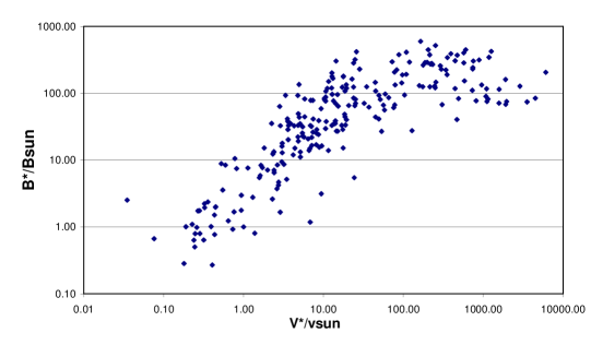
Figure 1: Magnetic field of stars (of late-type dwarfs) calculated from their X-ray emission, versus their rotation velocity.

IV Summary

We have developped a statistical theory of axisymetric MHD equations generalizing the 2D approach by Jordan97 . We derived the velocity and magnetic field distribution, and computed the corresponding equilibrium profiles for the mean flow. Like in the 2D case, the fluctuations around the mean field are found Gaussian, an universal feature connected to the conservation of the Casimirs under the coarse-graining. The equilibrium profiles are characterized by an alignment of the velocity and magnetic field, which is broken when the angular momentum conservation is taken into account. The statistical equilibrium profiles are found to correspond to profiles obtained under minimization of energy subject to the constraints. Thus, in the MHD case, in the presence of a coarse-graining (or a small viscosity), the energy is dissipated while the Helicity, the angular momentum and the Casimirs are approximately conserved (hydromagnetic selective decay). In particular, $\overline{E}=\frac{1}{2}\int\overline{{U}^{2}+{B}^{2}}d{\bf x}\neq\frac{1}{2}\int(\bar{U}^{2}+\bar{B}^{2})d{\bf x}$ because part of energy goes into fine grained fluctuations $E_{fluct}=\overline{E}-E_{m.f.}$. Therefore, the metaequilibrium state minimizes $E$ at fixed $I$, $H_{m}$, $H_{c}$ and $L$. This can be justified in the “classical case” (section III.3.1) where we showed that the fraction of kinetic energy going into the fluctuating part of the fields was higher than that of the other quantities, namely the magnetic energy and the cross-helicity. The “rotating case” (section III.3.2) requires more algebra and is left for further study.

In contrast, in the 2D hydrodynamical case, the Casimirs are fragile quantities (because they are expressed as function of the vorticity which is not an integral quantity as the magnetic potential is) and thus are altered by the coarse-graining procedure. This is true in particular for a special class of Casimirs $H=-\int C(\omega)d{\bf x}$, called $H$-functions, constructed with a convex function $C$ such that $C^{\prime\prime}>0$. This leads to two very different behaviors of hydrodynamical turbulence compared to the hydromagnetic one. First, the H-functions calculated with the coarse-grained vorticity $\overline{\omega}$ increase with time while the circulation and energy are approximately conserved (hydrodynamic selective decay). Thus, the metaequilibrium state maximizes one of the $H$-functions at fixed $E$ and $\Gamma$. For example, Chavanis and Sommeria jfm1 showed that in the limit of strong mixing (or for gaussian fluctuations), the quantity to maximize is minus the enstrophy, giving some mathematical basis to an (inviscid) “minimum enstrophy principle”. In this context, $\overline{\Gamma}_{2}=\int\overline{\omega^{2}}d{\bf x}\neq\int\bar{\omega}^{2}d{\bf x}$ because part of enstrophy goes into fine-grained fluctuations $\Gamma_{fluct}=\bar{\Gamma}_{2}-\Gamma_{2}^{m.f.}$. However, for more general situations, the $H$-function that is maximized at metaequilibrium is non-universal and can take a wide diversity of forms as discussed by Chavanis Chavanis03 . Due to their resemblance with entropy functionals (they increase with time, one is maximum at metaequilibrium,…), and because they generally differ from the Boltzmann entropy $S_{B}=-\int\omega\ln\omega d{\bf x}$, the $H$-functions are sometimes called “generalized entropies” Chavanis03 . From the statistical mechanics point of view, there is an infinite number of constraints (depending on the micro scale fields) to take into acccount when deriving the Gibbs state. Consequently, the shape of the fluctuations is not universal. This is why the $H$-function that is maximized at metaequilibrium is also non-universal. However, if the distribution of fluctuations is imposed by some external mechanism (e.g., a small-scale forcing) as suggested by Ellis et al. ellis , the functional $S[\overline{\omega}]$ is now a well-determined functional determined by the Gibbs state and the prior vorticity distribution ellis ; Chavanis03 .

Our computation can provide interesting insight regarding dynamo saturation. It is however limited by its neglect of dissipation and forcing mechanism. It would therefore be interesting to generalize this kind of approach to more realistic systems. In that case, the entropy might not be the relevent quantity anymore, but rather the turbulent transport, or the entropy production Dewar03 .

*

Appendix A Curl operators

Following Jordan and Turkington, we define

$${\rm curl}{\bf B} = (\nabla\times{\bf B})\cdot{\bf e}_{\theta}$$ (46)

$${\bf Curl}A = \nabla\times(A\,{\bf e}_{\theta})$$

for any vector ${\bf B}$ and scalar $A$. It is straightforward to show that we have the following relations:

$${\rm curl}{\bf Curl}(\frac{A}{r}) = -r\Delta_{*}A$$ (47)

$$\int A\ {\rm curl}{\bf B}\ d{\bf x} = \int{\bf Curl}A\cdot{\bf B}\ d{\bf x}$$ (48)

Setting $A={\rm Curl}^{-1}{\bf B}^{\prime}$ and ${\rm curl}{\bf B}=A^{\prime}$ in the last identity, we get

$$\int{\rm Curl}^{-1}{\bf B}^{\prime}\ A^{\prime}\ d{\bf x}=\int{\bf B}^{\prime}\cdot{\bf curl}^{-1}A^{\prime}\ d{\bf x}$$ (49)

References

- (1) A. Gailitis et al., Phys. Rev. Lett. 86, 3024 (2001).
- (2) R. Stieglitz and U. Müller, Phys. Fluids 13, 561 (2001).
- (3) F. Pétrélis and S. Fauve, Eur. Phys. J. B, 22, 273 (2001).
- (4) V. Archontis, PhD University of Copenhagen (2000).
- (5) L. Onsager, Nuovo Cimento Suppl. 6, 279 (1949).
- (6) D. Montgomery and G. Joyce, Phys. Fluids 17, 1139 (1974).
- (7) J. Miller, Phys. Rev. Lett. 65, 2137 (1990); J. Miller, P.B. Weichman and M.C. Cross, Phys. Rev. A 45, 2328 (1992).
- (8) R. Robert and J. Sommeria, J. Fluid Mech. 229, 291 (1991).
- (9) E. T. Jaynes, Phys. Rev 106, 620 (1957).
- (10) P.-H. Chavanis and J. Sommeria, J. Fluid Mech 314, 267 (1996).
- (11) D. Lynden-Bell, Mon. Not. R. Astron. Soc. 136, 101 (1967).
- (12) P.-H. Chavanis, in Dynamics and Thermodynamics of Systems with Long Range Interactions, edited by T. Dauxois, S. Ruffo, E. Arimondo, and M. Wilkens, Lecture Notes in Physics Vol. 602 (Springer, New York, 2002), preprint, cond-mat/0212223.
- (13) R. Ellis, K. Haven and B. Turkington, Nonlinearity 15, 239 (2002).
- (14) P.-H. Chavanis, Phys. Rev. E 68, 36108 (2003).
- (15) R. Jordan and B. Turkington, J. Stat. Phys., 87, 661 (1997).
- (16) L. Woltjer, Astrophys. J 130, 400 (1959).
- (17) S. Chandrasekhar, Proc. Nat. Acad. Sci. 44, 842 (1958).
- (18) D. D. Holm, J. E. Mardsen, T. Ratiu and A. Weinstein, Phys. Rep. 123, 1 (1985).
- (19) M. Steenbeck, F. Krause and K.-H. Rädler, Z. Naturforsch., Teil A, 21, 369 (1966).
- (20) A. Pouquet, U. Frisch and J. Leorat, J. Fluid Mech., 77, 321 (1976).
- (21) R. Robert and J. Sommeria, Phys. Rev. Lett., 69, 2776 (1992).
- (22) C. E. Shanon and W. Weaver, The mathematical theory of communication (University of Illinois Press, Urbana, 1949).
- (23) J. L. Lumley, Stochastic tools in turbulence (Academic Press, 1970).
- (24) D. Biskamp, Nonlinear Magnetohydrodynamics (CUP, 1993), Chap. 7 Sec. 3.
- (25) R. M. Kinney and J. C. Mc Williams, Phys. Rev. E 57, 7111 (1998).
- (26) R. Dewar, J. Phys. A 36, 631 (2003).