Theory of space-charge waves on gradient-profile relativistic electron beam:
an analysis in propagating eigenmodes

Abstract

We developed an exact analytical treatment for space-charge waves within a relativistic electron beam in terms of (self-reproducing) propagating eigenmodes. This result is of obvious theoretical relevance as it constitutes one of the few exact solution for the evolution of charged particles under the action of self-interactions. It also has clear numerical applications in particle accelerator physics where it can be used as the first self-consistent benchmark for space-charge simulation programs. Today our work is of practical relevance in FEL technology in relation with all those schemes where an optically modulated electron beam is needed and with the study of longitudinal space-charge instabilities in magnetic bunch compressors.

I Introduction

The evolution problem for a collection of charges under the action of their own fields when certain initial conditions are given is, in general, a formidable one. Numerical methods are often the only way to obtain an approximate solution, while there are only a few cases in which finding an exact treatment is possible.

In this paper we report a fully self-consistent solution to one of these problems, namely the evolution of a relativistic electron beam under the action of its own fields in the (longitudinal) direction of motion. The problem of longitudinal space-charge oscillations has been, so far, solved only from an electrodynamical viewpoint ROSE , or using limited one-dimensional models PLA2 . On the contrary, in our derivation the beam, which is assumed infinitely long in the longitudinal direction, is accounted for any given radial dependence of the particle distribution function.

An initial condition is set so that the beam is considered initially modulated in energy and density at a given wavelength. When the amplitude of the modulation is small enough the evolution equation can be linearized. An exact solution can be found in terms of an expansion in (self-reproducing) propagating eigenmodes.

Our findings are, in first instance, of theoretical importance since they constitute one of the few exact solutions known up to date to the problem of particles evolving under the action of their own fields.

Next to theoretical and academical interest of our study we want to emphasize here its current relevance to applied physics and technology. For example, particle accelerator physics in general and FEL physics in particular make large use of simulation codes (see for instance SIMS ; TDRD ; CDRS ) in order to obtain the influence of space-charge fields on the beam behavior. Yet, these codes are benchmarked against exact solutions of the electrodynamical problem alone (i.e. solutions of Poisson equation) and only recently PLA2 partial attempts have been made to benchmark them against some analytical model accounting for the system evolution. However, such attempts are based on one-dimensional theory which can only give some incomplete result. On the contrary, we claim that our findings can be used as a standard benchmark for any space-charge code from now on.

To give some up-to-date example of practical applications (besides, again, theoretical and numerical importance) we wish to underline that our results are of relevance to an entire class of problems arising in state-of-the-art FEL technology. In fact, several applications rely on feeding (optically) modulated electron beams into an FEL. For instance, optical seeding is a common technique for harmonic generation MOD0 . Moreover pump-probe schemes have been proposed that couple the laser pulse out of an X-ray FEL with an optical laser. To solve the problem of synchronization between the two lasers a method has been proposed, which makes use of a single optically modulated electron beam in order to generate both pulses. This proposal relies on the passage of this electron beam through an X-ray FEL and an optically tuned FEL MOD1 : given the parameters of the system, plasma oscillations turn out to be a relevant effect to be accounted for. It is also worth to mention, as another example, the relevance of plasma oscillation theory in the understanding of practical issues like longitudinal space-charge instabilities in high-brightness linear accelerators. High-frequency components of the bunch current spectrum (at wavelengths much shorter than the bunch length) can induce, through self-interaction, energy modulation within the electron beam which is then converted into density modulation when the beam passes through a magnetic compression chicane, thus leading to beam microbunching and break up. When longitudinal space-charge is the self-interaction driving the instability (see MICR ), one is interested to know with the best possible accuracy how plasma oscillations modulate the bunch, in energy and density, before the compression chicane.

Our calculations can be applied to these cases directly or in support to macroparticle simulations thus providing outcomes of immediate practical importance.

Throughout this paper we will make use of $cgs$ units. Our work is organized as follows. Next to this Introduction, in Section II, we pose the problem in the form of an integro-differential equation which makes use of naturally normalized quantities. In Section III we present our main theoretical results. In the following Section IV we describe some applications and important exemplifications of the obtained results, including the role of the initial condition. Finally, in Section V we come to conclusions.

II Theory

II.1 Position of the problem

We are interested in developing a theory to describe longitudinal plasma waves in a relativistic electron beam. In order to do so we have to find a way to translate in mathematical terms the idea of dealing with the longitudinal dynamics only, while keeping intact the general three-dimensional description of the system (electromagnetic fields and particle distribution).

Immediately related with the development of a theory, is its range of applicability. The idea of selecting longitudinal dynamics translates from a physical viewpoint in the assumption that the longitudinal space-charge fields, alone, describe the system evolution. This corresponds to a situation with physical parameters tuned in such a way that, on the time-scale of a longitudinal plasma oscillation, transverse dynamics does not play a role.

One may, of course, devise different methods to select the longitudinal dynamics alone: actually he will come up with some ideal approximation of what real focusing systems in modern linear accelerators do, provided that the $\beta$-functions are large enough with respect to the plasma wavelength.

Whatever the practical or ideal mean chosen to select longitudinal dynamics such a choice translates, from a mathematical viewpoint, in the choice of dynamical variables along the direction of motion only, while transverse coordinates enter purely as parameters in the description of the fields and of the particle distribution.

Our beam is initially modulated at some wavelength $\lambda_{m}$, in density and energy. This is no restriction because, as said in Section I, the modulation amplitude is considered small enough so that we can linearize the evolution equation. Then, a Fourier analysis of any perturbation in energy and density is customary. Once the modulation wavelength $\lambda_{m}$ has been fixed, it is natural to define the phase $\psi=\omega_{m}\left(z/v_{z}(\mathcal{E}_{0})-t\right)$, where $v_{z}(\mathcal{E}_{0})\sim c$ is the longitudinal electron velocity at the nominal beam kinetic energy $\mathcal{E}_{0}=(\gamma-1)mc^{2}$, $\omega_{m}=2\pi v_{z}/\lambda_{m}$, $t$ is the time and $z$ the longitudinal abscissa. Upon this, and after what has been said about the choice of longitudinal dynamics, it is appropriate to operate in energy-phase variables $(P,\psi)$, $P$ being the deviation from the nominal energy.

In this spirit the total derivative of the phase $\psi$ is given by:

$${d\psi\over{dz}}={\partial\psi\over{\partial z}}+{\partial\psi\over{\partial t}}{dt\over{dz}}={\omega_{m}\over{v_{z}(\mathcal{E}_{0})}}-{\omega_{m}\over{v_{z}(\mathcal{E})}}~{}.$$ (3)

Now, if we assume that the particle energy is not significantly different from the nominal energy we can expand $v(\mathcal{E})$ in $\mathcal{E}$ around $\mathcal{E}_{0}$. Keeping up to second order terms in $\mathcal{E}$ and using the definition of $P$ we find

$${d\psi\over{dz}}={\omega_{m}P\over{c\gamma_{z}^{2}\mathcal{E}_{0}}}~{},$$ (4)

where we took advantage of the fact that $(dv_{z}/d\mathcal{E})\mid_{\mathcal{E}=\mathcal{E}_{0}}\simeq c/(\gamma_{z}^{2}\mathcal{E}_{0}$), where $\gamma_{z}=(1-v_{z}(\mathcal{E}_{0})^{2}/c^{2})^{-1/2}$. Note that, here, we distinguish from the very beginning between $\gamma$ and $\gamma_{z}$ (or $v$ and $v_{z}$). In fact our theory can be applied to the case of an electron beam in vacuum as well as to the case of a beam under the action of external electromagnetic fields, for example in an undulator: in the first situation $\gamma=\gamma_{z}$, strictly, while in the latter they obviously have different values.

The full derivative of $P$ is simply given by

$${dP\over{dz}}=-eE_{z}~{},$$ (5)

where $E_{z}(z,\psi)$ is the space-charge field in the $z$ direction. Eq. (4) and Eq. (5) are the equation of motion for our system and they can be interpreted as Hamilton canonical equations corresponding to the Hamiltonian $H(\psi,P,z)$:

$$H=e\int{d\psi E_{z}}+{\omega_{m}\over{2c\gamma_{z}^{2}}}{P^{2}\over{\mathcal{E}_{0}}}~{}.$$ (6)

In this sense, Eq. (6), alone, defines our theory. The bunch density distribution will be then represented by the density $f=f(\psi,P,z;\bm{r_{\bot}})$, where the semicolon separates dynamical variables from parameters and it will be subjected to the (Vlasov) evolution equation

$${\partial f\over{\partial z}}+{\partial H\over{\partial P}}{\partial f\over{\partial\psi}}-{\partial H\over{\partial\psi}}{\partial f\over{\partial P}}=0~{}$$ (7)

with appropriate initial condition at $z=0$. Here we are interested in a beam initially modulated in energy and density; moreover, as said in Section I, the modulation must be small enough to ensure that linearization of Eq. (7) is possible. Thus we will take $f(\psi,P,z;\bm{r_{\bot}})_{\mid_{z=0}}=f_{0}(P;\bm{r_{\bot}})+f_{1}(\psi,P,z;\bm{r_{\bot}})_{\mid_{z=0}}$. $f_{0}$ is a so called unperturbed solution of the evolution equation Eq. (7), and it does not depend on $z$, while $f_{1}$ is known as the perturbation; it is understood that, in order to be in the linear regime, $f_{1}\ll f_{0}$ for any value of dynamical variables or parameters. In the following we assume that the dynamical variable $P$ and the parameter $\bm{r_{\bot}}$ are separable in $f_{0}$ so that we may write $f_{0}(P;\bm{r_{\bot}})=n_{0}(\bm{r_{\bot}})F(P)$, where the local energy spread function $F(P)$ is considered normalized to unity. The initial modulation can be written as a sum of density and energy modulation terms: $f_{1}(\psi,P,z;\bm{r_{\bot}})_{\mid}{{}_{z=0}}=f_{1d}(\psi,P;\bm{r_{\bot}})+f_{1e}(\psi,P;\bm{r_{\bot}})$.

On the one hand $f_{1d}$ is responsible for a pure density modulation and can be written as

$$f_{1d}(\psi,P,z;\bm{r_{\bot}})=a_{1d}(\bm{r_{\bot}})F(P)\cos(\psi)~{},$$ (8)

where we set to zero an unessential, initial modulation phase.

On the other $f_{1e}$ is responsible for a pure energy modulation and can be assumed to be

$$f_{1e}(\psi,P,z;\bm{r_{\bot}})=a_{1e}(\bm{r_{\bot}}){dF\over{dP}}\cos(\psi+\psi_{0})~{},$$ (9)

where $\psi_{0}$ is an initial (relative) phase between density and energy modulation. Finally it is convenient to define complex quantities $\tilde{f}_{1d}=a_{1d}F$, and $\tilde{f}_{1e}=a_{1e}({dF}/{dP})e^{i\psi_{0}}$ so that ${f}_{1_{\mid}{{}_{z=0}}}=(\tilde{f}_{1d}+\tilde{f}_{1e})e^{i\psi}+CC$. In the linear regime, then, one can write $f_{1}(\psi,P,z;\bm{r_{\bot}})=\tilde{f}_{1}(P,z;\bm{r_{\bot}})e^{i\psi}+CC$. Further definition of $\tilde{E}_{z}=\tilde{E}(z;\bm{r_{\bot}})$ in such a way that $E_{z}=\tilde{E}_{z}e^{i\psi}+\tilde{E}_{z}^{*}e^{-i\psi}$ allows one to write down the Vlasov equation, Eq. (7), linearized in $\tilde{f}_{1}$:

$${\partial\tilde{f}_{1}\over{\partial z}}+i{\omega_{m}P\over{c\gamma_{z}^{2}\mathcal{E}_{0}}}\tilde{f}_{1}-e\tilde{E}_{z}{\partial f_{0}\over{\partial P}}=0~{}.$$ (10)

Eq. (10) is far from being the final form of the evolution equation, since we still have to couple it with Maxwell equations, which constitute the electrodynamical part of the problem. However an integral representation of $\tilde{f}_{1}$ can be given at this stage:

$$\tilde{f}_{1}=\tilde{f}_{1_{\mid_{z=0}}}e^{-{i\omega_{m}Pz\over{c\gamma_{z}^{2}\mathcal{E}_{0}}}}+en_{0}{dF\over{dP}}\int_{0}^{z}{dz^{\prime}\tilde{E}_{z}e^{i{\omega_{m}P\over{c\gamma_{z}^{2}\mathcal{E}_{0}}}(z^{\prime}-z)}}~{}.$$ (11)

Let us now introduce the longitudinal current density $j_{z}(z;\bm{r_{\bot}})=-j_{0}(\bm{r_{\bot}})+\tilde{j}_{1}e^{i\psi}+\tilde{j}_{1}^{*}e^{-i\psi}$, where $j_{0}(\bm{r_{\bot}})\simeq ecn_{0}(\bm{r_{\bot}})$ and $\tilde{j}_{1}\simeq-ec\int_{-\infty}^{\infty}dP\tilde{f}_{1}$. Eq. (11) can be integrated in $P$ thus giving

$$\tilde{j}_{1}=-ec\int_{-\infty}^{\infty}dP\left(a_{1d}F+a_{1e}{dF\over{dP}}e^{i\psi_{0}}\right)e^{-i{\omega_{m}Pz\over{c\gamma_{z}^{2}\mathcal{E}_{0}}}}$$ (12)

$$-ej_{0}\int_{0}^{z}dz^{\prime}\left[\tilde{E}_{z}\int_{-\infty}^{\infty}dP{dF\over{dP}}e^{i{\omega_{m}P\over{c\gamma_{z}^{2}\mathcal{E}_{0}}}(z^{\prime}-z)}\right]~{}.$$ (13)

The next step is to present the equation for the electric field $\tilde{E}_{z}$ which, coupled with Eq. (13), will describe the system evolution in a self-consistent way.

We start with the inhomogeneous Maxwell equation for the z-component of the electric field

$$\nabla^{2}E_{z}-{1\over{c^{2}}}{\partial^{2}E_{z}\over{\partial t^{2}}}=4\pi{\partial\rho_{e}\over{\partial z}}+{4\pi\over{c^{2}}}{\partial j_{z}\over{\partial t}}~{},$$ (14)

where $\rho_{e}$ is the electron charge density. Remembering the definition of complex quantities $\tilde{E}_{z}$ and $\tilde{j}_{1}$ and accounting for the fact that $\rho_{e}\simeq j_{z}/v_{z}$ one can rewrite Eq. (14) as

$$\nabla_{\bot}^{2}\left(\tilde{E}_{z}e^{i\psi}\right)+{\partial^{2}\tilde{E}_{z}e^{i\psi}\over{\partial z^{2}}}-{1\over{c^{2}}}{\partial^{2}\tilde{E}_{z}e^{i\psi}\over{\partial t^{2}}}$$ (15)

$$={4\pi\over{v_{z}}}{\partial\tilde{j}_{1}e^{i\psi}\over{\partial z}}+{4\pi\over{c^{2}}}{\partial\tilde{j}_{1}e^{i\psi}\over{\partial t}}~{},$$ (16)

where $\nabla_{\bot}^{2}$ is the Laplacian operator over transverse coordinates. Explicit calculations of partial derivatives with respect to $t$ and $z$ give

$${\partial^{2}\tilde{E}_{z}e^{i\psi}\over{\partial z^{2}}}=\left({\partial^{2}\tilde{E}_{z}\over{\partial z^{2}}}+2i{\omega_{m}\over{v_{z}}}{\partial\tilde{E}_{z}\over{\partial z}}-{\omega_{m}^{2}\over{v_{z}^{2}}}\tilde{E}_{z}\right)e^{i\psi}~{},$$ (17)

$${\partial^{2}\tilde{E}_{z}e^{i\psi}\over{\partial t^{2}}}=-\omega_{m}^{2}\tilde{E}_{z}e^{i\psi}~{},$$ (18)

$${\partial\tilde{j}_{1}e^{i\psi}\over{\partial z}}={\partial\tilde{j}_{1}\over{\partial z}}e^{i\psi}+i{\omega_{m}\over{v_{z}}}\tilde{j}_{1}e^{i\psi}~{},$$ (19)

$${\partial\tilde{j}_{1}e^{i\psi}\over{\partial t}}=-i\omega_{m}\tilde{j}_{1}e^{i\psi}~{}.$$ (20)

Substitution back into Eq. (16) yields ($v_{z}\simeq c$):

$$\nabla_{\bot}^{2}\tilde{E}_{z}+{\partial^{2}\tilde{E}_{z}\over{\partial z^{2}}}+2i{\omega_{m}\over{v_{z}}}{\partial\tilde{E}_{z}\over{\partial z}}-{\omega_{m}^{2}\tilde{E}_{z}\over{\gamma_{z}^{2}c^{2}}}$$ (21)

$$={4\pi\over{v_{z}}}{\partial\tilde{j}_{1}\over{\partial z}}+{4\pi i\omega_{m}\over{\gamma_{z}^{2}c^{2}}}\tilde{j}_{1}~{}.$$ (22)

It is reasonable to assume that the envelope of fields and currents vary slowly enough over the $z$ coordinate, in order to neglect first and second derivatives with respect to $z$ in Eq. (22). Mathematically, this corresponds to the requirements

$${\left|\partial\tilde{E}_{z}\over{\partial z}\right|\ll{k_{m}\over{2\gamma_{z}^{2}}}{\left|\tilde{E}_{z}\right|}}~{},$$ (23)

$${\left|\partial^{2}\tilde{E}_{z}\over{\partial z^{2}}\right|\ll{k^{2}_{m}\over{\gamma_{z}^{2}}}{\left|\tilde{E}_{z}\right|}}~{}$$ (24)

and

$${\left|\partial\tilde{j}_{1}\over{\partial z}\right|\ll{k_{m}\over{\gamma_{z}^{2}}}{\left|\tilde{j}_{1}\right|}}~{},$$ (25)

where we introduced the wave number $k_{m}=2\pi/\lambda_{m}$. We note that $2\gamma^{2}_{z}\lambda_{m}$ is, roughly, the field formation length: by imposing conditions (23), (24) and (25) we are requiring that the characteristic lengths of variation for current, field and its derivative are much longer than the field formation length (actually condition (24) over the variation of the field derivative already included in condition (23), since $\gamma_{z}^{2}\gg 1$): this simply means that we can neglect retardation effects or, in other words, that the fields are known at a certain time, when the charge distribution are known at the same time. This assumption is not a restriction and it is verified in all cases of practical interest. Then Eq. (22) is simplified to

$$\nabla_{\bot}^{2}\tilde{E}_{z}-{\omega_{m}^{2}\tilde{E}_{z}\over{\gamma_{z}^{2}c^{2}}}={4\pi i\omega_{m}\over{\gamma_{z}^{2}c^{2}}}\tilde{j}_{1}~{},$$ (26)

which forms, together with Eq. (13), a self-consistent description for our system.

Similarity techniques can be now used in order to obtain a dimensionless version of Eq. (13) and Eq. (26). First note that the dependence of $j_{0}$ on the transverse coordinates can be expressed, in all generality, as

$$j_{0}=I_{0}S_{0}(\bm{r_{\bot}}/r_{0})\left[\int S_{0}(\bm{r_{\bot}}/r_{0})d\bm{r_{\bot}}\right]^{-1}~{},$$ (27)

where $I_{0}$ is the beam current, $r_{0}$ the transverse profile parameter (i.e. the typical transverse size of the beam), $S_{0}$ the transverse profile function of the beam and the integral in $d\bm{r_{\bot}}$ is calculated over all the transverse plane. Furthermore it is understood that the normalization of $S_{0}$ is chosen is such a way that $S_{0}(\bm{0})=1$. It is then customary to introduce the current density parameter $J_{0}=I_{0}\left[\int S(\bm{r_{\bot}}/r_{0})d\bm{r_{\bot}}\right]^{-1}$ so that we can define quite naturally the dimensionless current densities $\hat{j}_{0}=j_{0}/J_{0}\equiv S_{0}(\bm{r_{\bot}}/r_{0})$ and $\hat{j}_{1}=\tilde{j}_{1}/J_{0}$. It follows from Eq. (26) that the electric field should be normalized to $E_{0}=4\pi J_{0}/\omega_{m}$, which suggests the definition $\hat{E}_{z}=\tilde{E}_{z}/E_{0}$. For the normalization of the transverse coordinates we use ${\bf{\hat{r}}}=\bm{r_{\bot}}/r_{0}$ so that one is naturally guided by Eq. (26) to introduce the transverse size parameter

$$q=k_{m}r_{0}/\gamma_{z}~{}.$$ (28)

Eq. (26) can now be written in its final dimensionless form:

$$\hat{\nabla}_{\bot}^{2}\hat{E}_{z}-q^{2}\hat{E}_{z}=iq^{2}\hat{j}_{1}~{},$$ (29)

where $\hat{\nabla}_{\bot}^{2}$ is the Laplacian operator with respect to normalized transverse coordinates.

By analyzing Eq. (13) and using the normalized quantities defined above we recover a dimensionless variable $\hat{z}=\Lambda_{P}z$, where $\Lambda_{P}$ is given by

$$\Lambda_{P}=\left[4I/(I_{A}r_{0}^{2}\gamma\gamma_{z}^{2})\right]^{1/2}~{},$$ (30)

$I_{A}=mc^{3}/e$ being the Alfven current.

Using Eq. (30) and looking now at the exponential factors in Eq. (13) it is straightforward to introduce the dimensionless energy deviation $\hat{P}=P/(\rho\mathcal{E}_{0})$, $\rho$ being defined by

$$\rho={\Lambda_{p}\gamma_{z}^{2}\over{k_{m}}}~{}.$$ (31)

From the definition of $\hat{P}$ it follows immediately that the factor $\rho\mathcal{E}_{0}$ is a natural measure for energy deviations. The rms energy spread $\langle(\Delta\mathcal{E})^{2}\rangle$ can be measured by the dimensionless parameter

$$\hat{\Lambda}_{T}^{2}={\langle(\Delta\mathcal{E})^{2}\rangle\over{\rho^{2}\mathcal{E}_{0}^{2}}}~{}.$$ (32)

The local energy spread distribution $F(P)$ was defined as normalized to unity, so that it is customary to introduce $\hat{F}(\hat{P})$ as the distribution function in the reduced momentum $\hat{P}$ also normalized to unity. For example, when the energy spread is a gaussian we have $\hat{F}(\hat{P})=(2\pi\hat{\Lambda}_{T}^{2})^{-1/2}e^{-\hat{P}^{2}/(2\hat{\Lambda}_{T}^{2})}$. When $\hat{\Lambda}_{T}^{2}\ll 1$ our beam can be considered cold meaning that $\hat{F}(\hat{P})\simeq\delta(\hat{P})$. However note that, in order to specify quantitatively the range of validity of the cold beam assumption with respect to the values of $\hat{\Lambda}_{T}^{2}$, one should first solve the more generic evolution problem for a non-cold beam and then study the limit for small values of $\hat{\Lambda}_{T}^{2}$.

Now Eq. (13) can be expressed in the final, dimensionless form:

$$\hat{j}_{1}=\int_{-\infty}^{\infty}d{\hat{P}}\left(\hat{a}_{1d}\hat{F}+\hat{a}_{1e}{d\hat{F}\over{d\hat{P}}}\right)e^{-i{\hat{P}}{\hat{z}}}$$ (33)

$$-S_{0}\int_{0}^{\hat{z}}d\hat{z}^{\prime}\left[\hat{E}_{z}\int_{-\infty}^{\infty}d\hat{P}{d\hat{F}\over{d\hat{P}}}e^{i{\hat{P}(\hat{z}^{\prime}-\hat{z})}}\right]~{},$$ (34)

where $\hat{a}_{1d}=-eca_{1d}/J_{0}$ and $\hat{a}_{1e}=-ece^{i\psi_{0}}a_{1e}/(J_{0}\rho\mathcal{E}_{0})$. One can combine Eq. (34) and Eq. (29) in order to obtain a single integrodifferential equation for $\hat{E}_{z}$ or, alternatively, an integral equation for $\hat{j}_{1}$.

As regards the description of the evolution in terms of $\hat{E}_{z}$, direct substitution of Eq. (34) in Eq. (29) yields immediately

$$\hat{\nabla}_{\bot}^{2}\hat{E}_{z}-q^{2}\hat{E}_{z}=iq^{2}\int_{-\infty}^{\infty}d{\hat{P}}\left(\hat{a}_{1d}\hat{F}+~{}\hat{a}_{1e}{d\hat{F}\over{d\hat{P}}}\right)e^{-i{\hat{P}}{\hat{z}}}$$ (35)

$$-iq^{2}S_{0}\int_{0}^{\hat{z}}d\hat{z}^{\prime}\left[\hat{E}_{z}\int_{-\infty}^{\infty}d\hat{P}{d\hat{F}\over{d\hat{P}}}e^{i{\hat{P}(\hat{z}^{\prime}-\hat{z})}}\right]~{}.$$ (36)

(37)

On the other hand, the description of our system in terms of $\hat{j}_{1}$ can be obtained first by solving Eq. (29) and then substituting the solution in Eq. (13). For the solution of Eq. (29) we can use the following result (see for example FELT ):

$$\hat{E}_{z}=-{iq^{2}\over{2\pi}}\int{d{\bf{\hat{r}_{\bot}^{(s)}}}\hat{j}_{1}K_{0}\left(q\mid{\bf{\hat{r}_{\bot}}}-{\bf{\hat{r}_{\bot}^{(s)}}}\mid\right)}~{},$$ (38)

where $K_{0}$ indicates the modified Bessel function of the second kind. Then, substitution in Eq. (34) yields

$$\hat{j}_{1}=\int_{-\infty}^{\infty}d{\hat{P}}\left(\hat{a}_{1d}\hat{F}+\hat{a}_{1e}{d\hat{F}\over{d\hat{P}}}\right)e^{-i{\hat{P}}{\hat{z}}}$$ (39)

$$+{iq^{2}\over{2\pi}}S_{0}\int_{0}^{\hat{z}}d\hat{z}^{\prime}\left[\int{d{\bf{\hat{r}_{\bot}^{(s)}}}\hat{j}_{1}K_{0}\left(q\mid{\bf{\hat{r}_{\bot}}}-{\bf{\hat{r}_{\bot}^{(s)}}}\mid\right)}\right.$$ (40)

$$\left.\times\int_{-\infty}^{\infty}d\hat{P}{d\hat{F}\over{d\hat{P}}}e^{i{\hat{P}(\hat{z}^{\prime}-\hat{z})}}\right]~{}.$$ (41)

Note that the description of the system in terms of fields or currents is completely equivalent. Using one or the other is only a matter of convenience; it will turn out in the following Sections that the description in terms of the fields is particularly suitable for analytical manipulations, while the description in terms of currents is advisable in case of a numerical approach.

It is interesting to explore the asymptote of Eq. (37) for $q\rightarrow\infty$. In this case one obtains the following simplified equation for the field evolution:

$$\hat{E}_{z}=-i\int_{-\infty}^{\infty}d{\hat{P}}\left(\hat{a}_{1d}\hat{F}+~{}\hat{a}_{1e}{d\hat{F}\over{d\hat{P}}}\right)e^{-i{\hat{P}}{\hat{z}}}$$ (42)

$$+iS_{0}\int_{0}^{\hat{z}}d\hat{z}^{\prime}\left[\hat{E}_{z}\int_{-\infty}^{\infty}d\hat{P}{d\hat{F}\over{d\hat{P}}}e^{i{\hat{P}(\hat{z}^{\prime}-\hat{z})}}\right]~{}.$$ (43)

In the case of a cold beam $\hat{F}(\hat{P})=\delta(\hat{P})$ and Eq. (43) transforms to

$$\hat{E}_{z}=-i\left(\hat{a}_{1d}+i\hat{a}_{1e}\hat{z}\right)+S_{0}\int_{0}^{\hat{z}}d\hat{z}^{\prime}\left(\hat{z}^{\prime}-\hat{z}\right)\hat{E}_{z}~{}.$$ (44)

Finally, after double differentiation with respect to $\hat{z}$ we get back the well-known pendulum equation for one-dimensional systems:

$${\partial^{2}\hat{E}_{z}\over{\partial\hat{z}^{2}}}+S_{0}\hat{E}_{z}=0~{}.$$ (45)

In this approximation, and in the particular case $S_{0}=1$, we recover the one-dimensional plasma wave number $\Lambda_{p}$, which agrees with the normalization $\hat{z}=\Lambda_{p}z$. It should be noted that such a normalization is natural in the limit $q\rightarrow\infty$ but it progressively loses its physical meaning as $q$ becomes smaller and smaller: of course, using our dimensionless equations for $q\ll 1$ will still yield correct results, because the equations are correct, but the normalization fits no more the physical feature of the system, in that case.

Eq. (43), which describes the system evolution in the limit $q\rightarrow\infty$, corresponds to the the one-dimensional case. We can use Eq. (43) and impose $\hat{z}=0$ thus getting the electromagnetic field at the beginning of the evolution, i.e. the solution of the electromagnetic problem in the limit $q\rightarrow\infty$:

$$\hat{E}_{z}=-i\hat{j}_{1\mid_{\hat{z}=0}}~{}.$$ (46)

This can be easily written in dimensional form as

$$E_{z}={4i\over{k_{m}r_{0}^{2}}}\left(-{I_{1}\over{c}}\right)~{},$$ (47)

where $j_{1}\simeq I_{1}/(\pi r_{0}^{2})$.

We can check Eq. (47) with already known results in scientific literature. In fact, the field generated by an electron beam modulated in density in free space can be easily calculated in the system rest frame (see e.g. ROSE and EEMF ). In the limit of a pancake beam (i.e. for large transverse dimension) the following impedance per unit length of drift has been found:

$$Z={4i\over{k_{m}r_{0}^{2}}}~{}.$$ (48)

The first factor on the right hand side of Eq. (47), which is the impedance per unit drift according to our calculations, is exactly the result in Eq. (48) which proves that our starting equation Eq. (37) can be used to solve correctly the electromagnetic problem in the case $q\rightarrow\infty$, as it must be.

Finally, before proceeding, it is worth to estimate the value of our parameters for some practical example and to see how our assumptions compare with an interesting case. Nowadays photo-injected LINACs, to be used as linear colliders or FEL injectors constitute cutting edge technology as regards electron particle accelerators. Currents of about $3~{}k$A with energy such that $\gamma\sim 10^{3}$ can be achieved together with quite a small energy spread $\langle(\Delta\mathcal{E})^{2}\rangle^{1/2}\sim 100~{}k$eV, radial dimensions of order $r_{0}\sim 100~{}\mu$m and a normalized emittance $\epsilon_{n}\sim 1$ mm mrad. In these conditions, a typical modulation wavelength of about $1~{}\mu$m will lead to a value of $q\sim 1$, which is well outside the region of applicability of the one-dimensional theory so that a generalized theory like the ours must be used. It is interesting to note that, by means of the definitions of $q$ and $\Lambda_{p}$, we can write $\rho=[I/(\gamma I_{A})]^{1/2}q^{-1}$: this suggests that a natural measure for the current is indeed $\gamma I_{A}$ which is, in practice, the Alfven-Lawson current (see ALFV , LAWS , OLSO ). In our numerical example $q\sim 1$ and the value of $\rho$ is actually determined by the ratio $I/(\gamma I_{A})\sim 2\cdot 10^{-4}$. As a result $\rho\sim 10^{-2}$: this means that our simplified Maxwell equation, Eq. (26), is valid up to an accuracy of $10^{-2}$. Moreover, in this case, $\hat{\Lambda}_{T}^{2}\sim 10^{-4}$ so that the cold beam case turns out to be of great practical interest. Finally $\epsilon_{n}\sim 1$ mm mrad. This corresponds, for $\gamma\sim 10^{3}$, to a betatron function $\beta_{f}\sim\gamma r_{0}^{2}/\epsilon_{n}\sim 10$ m. Our choice of considering the longitudinal motion alone is satisfied when the period of a plasma oscillation is much shorter than the period of a betatron oscillation, that is when $\Lambda_{p}\beta_{f}\gg 1$. It should be noted, though, that this estimation cannot have a rigorous mathematical background before a more comprehensive theory, including the effects of transverse dynamics, is developed: only then our present theory can be reduced to an asymptote of a more general situation, and conditions for its applicability can be derived in a rigorous way. Keeping this fact in mind, in our example $\Lambda_{p}\sim 3\cdot 10^{-1}$m^-1 which means $\Lambda_{p}\beta_{f}\sim 3$ signifying that this particular case is at the boundary of the region of applicability of our theory.

III Main result

Given Eq. (37) with appropriate initial conditions for $\hat{j}_{1_{\mid_{\hat{z}=0}}}$ it is possible to find an analytical solution to the evolution problem. The method is similar to the one used for the solution of the self-consistent problem in FEL theory (see DIFF ) and relies on the introduction of the Laplace transform of $\hat{E}_{z}$, namely:

$$\bar{E}(p,{\bf{\hat{r}_{\bot}}})=\int_{0}^{\infty}d\hat{z}e^{-p\hat{z}}\hat{E}_{z}~{},$$ (49)

with $Re(p)>0$. The advantage of the Laplace transform technique is that the evolution equation is transformed from the integrodifferential equation Eq. (37) into the following ordinary differential equation:

$$\left[\hat{\nabla}_{\bot}^{2}-q^{2}(1-i\hat{D}S_{0})\right]\bar{E}=iq^{2}\left(\hat{D}_{0}\hat{a}_{1d}+\hat{D}\hat{a}_{1e}\right)~{},$$ (50)

where

$$\hat{D}_{0}=\int_{-\infty}^{\infty}d\hat{P}{\hat{F}\over{p+i\hat{P}}}~{},$$ (51)

and

$$\hat{D}=\int_{-\infty}^{\infty}d\hat{P}{d\hat{F}/d{\hat{P}}\over{p+i\hat{P}}}$$ (52)

with the boundary conditions $\bar{E}\longrightarrow 0$ for $|{\bf{\hat{r}_{\bot}}}|\longrightarrow\infty$ and $\partial\bar{E}/\partial{\bf{\hat{r}_{\bot}}}\longrightarrow 0$ for $|{\bf{\hat{r}_{\bot}}}|\longrightarrow\infty$. We can rewrite Eq. (50) as

$$\mathcal{L}\bar{E}={f}~{},$$ (53)

having introduced

$$\mathcal{L}=\hat{\nabla}_{\bot}^{2}+\hat{g}({\bf{\hat{r}_{\bot}}},p)~{},$$ (54)

$${f}({\bf{\hat{r}_{\bot}}},p)=iq^{2}\left(\hat{D}_{0}\hat{a}_{1d}+\hat{D}\hat{a}_{1e}\right)~{}$$ (55)

and

$$\hat{g}({\bf{\hat{r}_{\bot}}},p)=-q^{2}(1-i\hat{D}S_{0})~{}.$$ (56)

Note that only Eq. (37) can benefit from the use of the Laplace transform but not the integral equation Eq. (41).

Eq. (53) is a nonhomogeneous, linear, second-order differential equation. We are interested in solving Eq. (53) for any given $p$ such that $Re(p)>0$. Solution is found if we can find the inverse of the operator $\mathcal{L}$, namely a Green function $\bar{G}$ obeying the given boundary conditions; in this case we simply have

$$\bar{E}=\int d{\bf{\hat{r}^{\prime}_{\bot}}}{\bar{G}}({\bf{\hat{r}_{\bot}}},{\bf{\hat{r}^{\prime}_{\bot}}})f({\bf{\hat{r}^{\prime}_{\bot}}})~{}.$$ (57)

III.1 Generic approach

Depending on the choice of $\hat{g}$, i.e. on the choice of $S_{0}$, $\hat{F}$ and $p$, the differential operator $\mathcal{L}$ can change its character completely making $\mathcal{L}$ more or less difficult to deal with. For example, the case of a self-adjoint operator is obviously a simple situation, since its eigenvalues are real and its eigenfunctions form a complete and orthonormal set for the space of squared-integrable functions $L^{2}$ (defined over the entire transverse plane through ${\bf{\hat{r}_{\bot}}}$) with respect to the internal product:

$$<h~{}|~{}g>=\int d{\bf{\hat{r}_{\bot}}}gh^{*}~{}.$$ (58)

Then, such a orthonormal set can be used to provide, quite naturally, an expansion for $\bar{G}$.

However, in the most general situation, $\mathcal{L}$ is not self-adjoint: to see this, it is sufficient to note that $\hat{g}$ is not real. As a result, the eigenvalues of $\mathcal{L}$ are not real, its eigenfunctions are not orthogonal with respect to the internal product in Eq. (58), we do not know wether the spectrum of $\mathcal{L}$ is discrete, completeness is not granted and we cannot prove the existence of a set of eigenfunctions either.

To the best of our knowledge there is no theoretical mean to really deal with our problem in full generality. When not self-adjoint operators are encountered in different branches of Physics (see, for example, KRIN and SIEG ) mathematical rigorousness is somehow relaxed assuming, rather than proving, certain properties of the operator. We will do the same here assuming, to begin, the existence of eigenfunction sets; then, as for example has been remarked in KRIN and SIEG one can consider, together with the spectrum of $\mathcal{L}$ defined by the eigenvalue problem:

$$\mathcal{L}\Psi_{j}=\Lambda_{j}\Psi_{j}$$ (59)

also the spectrum of its adjoint, defined by

$$\mathcal{L}^{*}{\Psi}_{j}^{*}=[\Lambda_{j}]^{*}{\Psi}_{j}^{*}~{}.$$ (60)

It can be shown by using the bi-orthogonality theorem BIOR that

$$<\Psi_{j}^{*}|{\Psi}_{i}>=\int d{\bf{\hat{r}_{\bot}}}\Psi_{j}\Psi_{i}=\delta_{ji}~{}.$$ (61)

In other words the sequence $\{\Psi_{j}\}_{j}$ admits $\{{\Psi}_{j}^{*}\}_{j}$ as a bi-orthonormal sequence. Then one has to assume completeness and discreteness of the spectrum so that the following expansion is correct:

$$\bar{G}=\sum_{j}|\bar{G}{\Psi}_{j}><\Psi_{j}^{*}|~{},$$ (62)

We ascribe to alternative theoretical approaches and numerical techniques the assessment of the validity region of this assumption, which should be ultimately formulated in terms of a restriction on the possible choices of $S_{0}$ and $\hat{F}$. In other words we give here a general method for solving our problem which is valid only under the fulfillment of certain assumptions, but we make clear that it is not possible, to the best of our knowledge, to strictly formulate the applicability region of this method in terms of properties of $S_{0}$ and $\hat{F}$ as it would be desirable.

With this in mind one can use the fact that $\bar{G}\equiv\mathcal{L}^{-1}$ and write

$$\bar{G}({\bf{\hat{r}_{\bot}}},{\bf{\hat{r}^{\prime}_{\bot}}})=\sum_{j}{\Psi_{j}({\bf{\hat{r}_{\bot}}})\Psi_{j}({\bf{\hat{r}^{\prime}_{\bot}}})\over{\Lambda_{j}}}~{}.$$ (63)

Finally, substituting Eq. (63) in Eq. (57) one gets

$$\bar{E}=\sum_{j}{\Psi_{j}({\bf{\hat{r}_{\bot}}})\over{\Lambda_{j}}}\int d{\bf{\hat{r}^{\prime}_{\bot}}}\Psi_{j}({\bf{\hat{r}^{\prime}_{\bot}}})f({\bf{\hat{r}^{\prime}_{\bot}}})~{}.$$ (64)

To find $\hat{E}_{z}$ we use the inverse Laplace transformation that is the Fourier-Mellin integral:

$$\hat{E}_{z}(\hat{z},{\bf{\hat{r}_{\bot}}})={1\over{2\pi i}}\int_{\alpha-i\infty}^{\alpha+i\infty}dp\bar{E}(p,{\bf{\hat{r}_{\bot}}})e^{p\hat{z}}~{},$$ (65)

where the integration path in the complex $p$-plane is parallel to the imaginary axis and the real constant $\alpha$ is positive and larger than all the real parts of the singularities of $\bar{E}$.

The application of the Fourier-Mellin formula comes with another, separate mathematical problem related with the ability of performing the integral in Eq. (65). One method to calculate the integral is to use numerical techniques and integrate directly over the path defined, on the complex $p$-plane, by $Re(p)=\alpha$.

Yet, there is some room for application of analytical techniques left. In fact, under the hypothesis that $\bar{E}$ is also defined, except for isolated singularities, as an analytical function on the left half complex $p$-plane and on the imaginary axis and under the hypotesis that $\bar{E}\rightarrow 0$ uniformly faster than $1/|p|^{k}$ for a chosen $k>0$ and for $\mathrm{Arg}(p)$ within $[\pi/2,3\pi/2]$ one could use Jordan lemma and close the integration contour of Eq. (65) by a semicircle at infinity on the left half complex $p$-plane. An obvious (and well-known) problem is that $\bar{E}$ is defined only for $Re(p)>0$ according to Eq. (49). Yet, if the border points at $Re(p)=0$ are regular points of $\bar{E}$ (except for isolated singularities) then one can consider the (unique) analytical continuation of $\bar{E}$ along the border, from the original domain of analyticity (i.e. the points $p$ with $Re(p)>0$ except for isolated singularities) to the entire complex plane (again, isolated singularity excluded). Then one can still apply Jordan lemma on the analytic continuation of $\bar{E}$ (provided that it obeys the other assumption), because the final result is the integral in Eq. (65) which is uniquely defined by the original function $\bar{E}$ for $Re(p)>0$.

The problem is trivially solved for the case of a cold beam because $\hat{F}=\delta(\hat{P})$ so that $\hat{D}_{0}=1/p$ and $\hat{D}=-i/p^{2}$. Then Eq. (64) defines indeed an analytic function in all points of the complex plane with the exception of $p=0$ and the points such that $\Lambda_{j}(p)=0$. All the hypothesis of Jordan lemma are verified and the method can be applied without any problem.

The situation is completely different in the case of a generic energy spread function $\hat{F}$. In fact by inspection of Eq. (51) and Eq. (52) one is immediately confronted with the fact that the integrands in $\hat{D}_{0}$ and $\hat{D}$ are, usually, singular at all the points of the imaginary axis $Re(p)=0$ since the integration in $\hat{P}$ is taken from $-\infty$ to $+\infty$. As a result the points $Re(p)=0$ are not regular points of $\bar{E}$ and $\bar{E}$ cannot be analytically continued through the border $Re(p)=0$.

This problem is the same encountered in the treatment of Landau damping (see LAND ). Of course one may follow the solution proposed by Landau and present particular definitions of $\hat{D}_{0}$ and $\hat{D}$ at $Re(p)=0$ that are

$$\hat{D}_{0}=\mathcal{(}P)\int_{-\infty}^{\infty}d\hat{P}{\hat{F}\over{p+i\hat{P}}}+\pi\hat{F}(ip)~{}~{}~{}~{}~{}Re(p)=0$$ (66)

and

$$\hat{D}=\mathcal{(}P)\int_{-\infty}^{\infty}d\hat{P}{d\hat{F}/d{\hat{P}}\over{p+i\hat{P}}}+\pi\hat{F}^{\prime}(ip)~{}~{}~{}~{}~{}Re(p)=0~{},$$ (67)

so that $D_{0}$ and $D$ are now regular for $Re(p)=0$ and can be (uniquely) continued at $Re(p)<0$ by

$$\hat{D}_{0}=\int_{-\infty}^{\infty}d\hat{P}{\hat{F}\over{p+i\hat{P}}}+2\pi\hat{F}(ip)~{}~{}~{}~{}~{}Re(p)<0$$ (68)

and

$$\hat{D}=\int_{-\infty}^{\infty}d\hat{P}{d\hat{F}/d{\hat{P}}\over{p+i\hat{P}}}+2\pi\hat{F}^{\prime}(ip)~{}~{}~{}~{}~{}~{}Re(p)<0~{}.$$ (69)

In this way the definition of $\bar{E}$ could be extended, except for isolated singularities, to an analytical function on the entire complex $p$-plane and, if $\hat{F}(\hat{P})$ behaves relatively well, Jordan lemma can be applied without further problems.

Yet, we think that the application of Landau’s prescription, i.e. the definition in Eq. (66) and Eq. (67) should be taken with extreme caution. As it is reviewed by Klimontovich KLIM and references therein, Landau’s method is equivalent to the introduction of additional assumptions on the system, namely the adiabatic switching on of the space-charge field at $t=-\infty$.

Another method equivalent to Landau’s consists, as has been remarked long ago by Lifshitz LIFT , in the introduction of a small dissipative term into the linearized Vlasov equation which ceases to be non-dissipative from the very beginning. The Vlasov equation is then solved by Fourier technique and the limit for a vanishing dissipating term is taken in the final result, which leads, in the end, to Landau’s result. Yet, the limit for a vanishing dissipation must be taken in the final formulas in order to recover Landau’s coefficient and not before. This means that Landau’s method consists in the introduction of additional assumptions regarding the system under study or equivalently, in changing the very nature of the equations describing our system (from non-dissipative to dissipative): therefore in practical calculations, we prefer to deal only with the case of a cold beam where the original non-dissipative nature of the system is maintained without problems, leaving the other case to future study. Such a viewpoint constitutes a restriction but as we have seen in the previous Section the cold beam case is practically quite an important issue: in this Section, we will present our results in full generality without fixing $\hat{F}$ but keeping in mind, however, all the warnings discussed before.

In any case and again, in all generality, we can say that wether or not the conditions of Jordan lemma are satisfied depends on the distribution $\hat{F}(\hat{P})$. In the case Jordan lemma is applicable one can find a closed, analytic expression for $\hat{E}_{z}$:

$$\hat{E}_{z}(\hat{z},{\bf{\hat{r}_{\bot}}})=\sum_{j}\Phi_{j}({\bf{\hat{r}_{\bot}}})e^{\lambda_{j}\hat{z}}\left[\left({d\Lambda_{j}(p)\over{dp}}\right)_{p=\lambda_{j}}\right]^{-1}$$ (70)

$$\times\int_{0}^{\infty}d{\bf{\hat{r}^{\prime}_{\bot}}}\Phi_{n}(\bf{\hat{r}^{\prime}_{\bot}})f({\bf{\hat{r}^{\prime}_{\bot}}},\lambda_{j})~{},$$ (71)

where $\Phi_{j}({\bf{\hat{r}_{\bot}}})=\Psi_{j}({\bf{\hat{r}_{\bot}}},p=\lambda_{j})$ and $\lambda_{j}$ are solutions of the equations:

$$\Lambda_{j}(p)=0~{}$$ (72)

or, which is the same, solution of Eq. (59) as $\Lambda_{j}=0$: from this viewpoint the functions $\Phi_{nj}$ constitute the kernel of the operator $\mathcal{L}$ and $\lambda_{j}$ are the values of $p$ such that $\mathcal{L}$ admits a non-empty kernel.

It is interesting to note that $\{\Phi_{j}\}_{j}$ is a subset of $\{\Psi_{j}\}_{j,p}$ naturally suited to expand any function of physical interest (the field $\hat{E}_{z}$). In this sense, one may say that the fields are subjected to constraints given by Maxwell equations, which are codified through the operator $\mathcal{L}$; these constraints are implicitly used during the anti-Laplace transform process, thus selecting only those $\{\Psi_{j}\}_{j,p}$ of physical interest. In this spirit, although $p$ is mathematically allowed to span over all the complex plane with $Re(p)>0$, only the particular values for which $p=\lambda_{j}$ have physical meaning in the final result.

An explicit expression for $({d\Lambda_{j}(p)/{dp}})_{p=\lambda_{j}}$ can be found. Using Eq. (61) and Eq. (59) we can write

$$\Lambda_{j}=\int d{\bf{\hat{r}_{\bot}}}\Psi_{j}\mathcal{L}\Psi_{j}~{}.$$ (73)

Then, differentiating Eq. (73) we have

$${d\Lambda_{j}\over{dp}}=\int d{\bf{\hat{r}_{\bot}}}{\partial g\over{\partial p}}\Psi_{j}^{2}$$ (74)

Our final result is therefore written as follows:

$$\hat{E}_{z}(\hat{z},{\bf{\hat{r}_{\bot}}})=\sum_{j}u_{j}\Phi_{j}({\bf{\hat{r}_{\bot}}})e^{\lambda_{j}\hat{z}}~{},$$ (75)

where the coupling factor $u_{j}$ is given by

$$u_{j}={\int d{\bf{\hat{r}^{\prime}_{\bot}}}\Phi_{j}({\bf{\hat{r}^{\prime}_{\bot}}})f({\bf{\hat{r}^{\prime}_{\bot}}},\lambda_{j})\over{~{}~{}~{}~{}\left[\int d{\bf{\hat{r}^{\prime}_{\bot}}}\left({\partial g\over{\partial p}}\right)\Psi_{j}^{2}\right]_{p=\lambda_{j}}}}~{}.$$ (76)

Eq. (75) describes the evolution of the system under the action of self-fields in a generic way, for any bunch transverse shape $S_{0}$, for any choice of local energy spread $\hat{P}$ and any initial condition (under the assumptions mentioned before). Our solution is indeed an analysis in (self-reproducing) propagating eigenmodes of the electric field.

We have seen that, due to the fact that $\mathcal{L}$ is in general not self-adjoint, the modes $\Psi_{j}$ are not orthogonal in the sense of Eq. (58) nor, as a consequence, $\Phi_{j}$ are. Moreover, even if $\Psi_{j}$ were orthogonal, $\Phi_{j}$ are chosen among the $\Psi_{j}$ at different values of $p$ so that orthogonality of $\Phi_{j}$ with respect to Eq. (58) is also not granted. It is possible, however, to formulate appropriate initial conditions to obtain a single propagating mode as a solution of our self-consistent problem. This demonstrates that single modes have physical meaning besides being mathematical tools for function decompositions.

Suppose, for example, that we wish to excite a single mode at fixed values of $j$. On the one hand Eq. (75) is simplified to

$$\hat{E}_{z}=u_{j}\Phi_{j}~{}e^{\lambda_{j}\hat{z}}$$ (77)

and, differentiating with respect to $z$, one also obtains

$${\partial\hat{E}_{z}\over{\partial\hat{z}}}=\lambda_{j}\hat{E}_{z}~{}.$$ (78)

On the other hand, the evolution equation, Eq. (37) at $\hat{z}=0$ reads:

$$\mathcal{O}\hat{E}_{z_{\mid_{\hat{z}=0}}}=iq^{2}\hat{a}_{1d}~{},$$ (79)

where we introduced

$$\mathcal{O}=\hat{\nabla}_{\bot}^{2}-q^{2}~{}.$$ (80)

The same Eq. (37) differentiated with respect to $\hat{z}$ and evaluated at $\hat{z}=0$ gives

$$\mathcal{O}\left({\partial\hat{E}_{z}\over{\partial\hat{z}}}\right)_{\mid_{\hat{z}=0}}=-q^{2}\hat{a}_{1e}~{},$$ (81)

which may be rewritten using Eq. (78) as:

$$\mathcal{O}\hat{E}_{z_{\mid_{\hat{z}=0}}}=-{q^{2}\over{\lambda_{j}}}~{}\hat{a}_{1e}~{}.$$ (82)

Finally, if $\hat{a}_{1e}\neq 0$, comparison of Eq. (82) and Eq. (79) gives:

$${\hat{a}_{1e}\over{\hat{a}_{1d}}}={-i\lambda_{j}}~{}.$$ (83)

Since for plasma oscillations $\lambda_{j}$ has to be imaginary, Eq. (83) fixes the phase $\psi_{0}=l\pi$ (with $l$ integer number). The actual shape of $\hat{a}_{1d}$ (and $\hat{a}_{1e}$) is obtained, modulus a multiplicative constant, by substitution of Eq. (77), calculated at $\hat{z}=0$, in Eq. (79) and it is fixed by the following condition:

$$\hat{a}_{1d}=\mathcal{O}(\Phi_{j})~{}.$$ (84)

We will now present some remarkable example of how to apply Eq. (75) and explore, in particular cases, the applicability region of our method.

We will start our exploration discussing the situation of an axis-symmetric beam which is still quite a generic one. Given the symmetry of the problem we will make use, from now on, of a cylindrical (normalized) coordinate system $(\hat{r},\phi,\hat{z})$, with obvious meaning of symbols.

Since $\hat{j}_{1}=\hat{j}_{1}(\hat{r},\hat{z},\phi)$, $\hat{E}_{z}=\hat{E}_{z}(\hat{r},\hat{z},\phi)$ and $f=f(\hat{r},p,\phi)$, it is convenient to decompose them in azimuthal harmonics according to

$$\hat{j}_{1}(\hat{z};\hat{r},\phi)=\sum_{n=-\infty}^{\infty}\hat{j}_{1}^{(n)}(z,\hat{r})e^{-in\phi}~{},$$ (85)

$$\hat{E}_{z}(\hat{z};\hat{r},\phi)=\sum_{n=-\infty}^{\infty}\hat{E}_{z}^{(n)}(\hat{z};\hat{r})e^{-in\phi}~{}$$ (86)

and

$$f(\hat{r},p,\phi)=\sum_{n=-\infty}^{\infty}f^{(n)}(\hat{r},p)e^{-in\phi}~{}.$$ (87)

Moreover, in cylindrical coordinates we have

$$\hat{\nabla}^{2}_{\bot}={1\over{\hat{r}}}{\partial\over{\partial\hat{r}}}\left[\hat{r}{\partial\over{\partial\hat{r}}}\right]+{1\over{r^{2}}}{\partial^{2}\over{\partial\phi^{2}}}~{}.$$ (88)

These definitions allow us to write our equations and results for the $n$-th azimuthal harmonic of the electric field. In this situation the operators $\mathcal{L}$ and $\mathcal{O}$ can be written as

$$\mathcal{L}={\partial^{2}\over{\partial\hat{r}^{2}}}+{1\over{\hat{r}}}{\partial\over{\partial\hat{r}}}-{n^{2}\over{\hat{r}^{2}}}+\hat{g}(\hat{r},p)~{},$$ (89)

where, now, $S_{0}=S_{0}(\hat{r})$ in the definition of $\hat{g}$ and

$$\mathcal{O}={\partial^{2}\over{\partial\hat{r}^{2}}}+{1\over{\hat{r}}}{\partial\over{\partial\hat{r}}}-\left(q^{2}+{n^{2}\over{\hat{r}^{2}}}\right)~{}$$ (90)

so that

$$\mathcal{L}\bar{E}^{(n)}={f}^{(n)}~{},$$ (91)

Having specialized our results to the axis-symmetric case it is worth to spend some words on the nature of the operator $\mathcal{L}$ in one particular case. As we have said at the beginning of this section, the case of a self-adjoint operator is a particularly blessed one. It is interesting to note that in the axis-symmetric case, when $S_{0}$, $\hat{F}$ and $p$ are such that $\hat{g}$ is real, we deal with a singular Sturm-Liouville problem as it is shown immediately by multiplying side by side by $\hat{r}$ Eq. (91). In fact, in this case $\mathcal{L}$ can be written in the usual form presented in Sturm-Liouville theory:

$$\mathcal{L}={\partial\over{\partial\hat{r}}}\left[\hat{r}{\partial\over{\partial\hat{r}}}\right]-{n^{2}\over{\hat{r}}}+\hat{r}\hat{g}(\hat{r},p)~{}.$$ (92)

In this case given the internal (axisisymmetric) product in $L^{2}$:

$$<h~{}|~{}g>=\int_{0}^{\infty}d\hat{r}\hat{r}gh^{*}~{},$$ (93)

self-adjointness condition for $\mathcal{L}$ is satisfied in the interval $[0,\infty)$ by all the functions in the linear space $\mathbb{S}$ which we define as the space of integrable-square functions not singular with their first derivatives at $\hat{r}=0$ and such that, for any $f,g$ chosen in $\mathbb{S}$ the following condition is satisfied:

$$\lim_{\hat{r}\rightarrow\infty}\hat{r}\left[g^{*}(\hat{r})f^{\prime}(\hat{r})-f(\hat{r})g^{\prime*}(\hat{r})\right]=0~{}.$$ (94)

Note that $\mathbb{S}$ is a subset of $L^{2}$.

This is of course a very particular situation, interesting to discuss but unfortunately not very useful in practise, since in order to solve our problem we still have to assume that Eq. (62) is correct for a generic $p$. When this assumption is made, in the axis-symmetric case our results Eq. (75) and Eq. (76) take the form

$$\hat{E}_{z}^{(n)}(\hat{z},\hat{r})=\sum_{j}u_{nj}\Phi_{nj}(\hat{r})e^{\lambda^{(n)}_{j}\hat{z}}~{},$$ (95)

where

$$u_{nj}(\hat{r})={\int_{0}^{\infty}d\hat{r}^{\prime}\hat{r}^{\prime}\Phi_{nj}f^{(n)}(\hat{r}^{\prime},\lambda_{j}^{(n)})\over{~{}~{}~{}~{}\left[\int_{0}^{\infty}d\hat{r}^{\prime}\hat{r}^{\prime}\left({\partial g\over{\partial p}}\right)\Psi_{nj}^{2}\right]_{p=\lambda^{(n)}_{j}}}}~{}.$$ (96)

Within this special situation we will now treat in detail the case of a stepped or parabolic transverse profile. Further on we will see how the solution for the stepped transverse profile can be used to obtain a semi-analytic solution for any transverse profile.

III.2 Stepped profile

Consider the case of a step function $S_{0}=1$ for $\hat{r}<1$ and $S_{0}=0$ for $\hat{r}\geq 1$. In this case $\hat{g}(\hat{r},p)$ inside the operator $\mathcal{L}$ is simply given by

$$\hat{g}(\hat{r},p)=\left\{\begin{array}[]{c}-q^{2}\left(1+{1\over{p^{2}}}\right)~{}~{}~{}~{}\hat{r}<1\\ -q^{2}~{}~{}~{}~{}~{}~{}~{}~{}~{}~{}~{}~{}~{}~{}~{}~{}~{}\hat{r}\geq 1\end{array}\right.~{},$$ (97)

Let us restrict to the assumption of a cold beam with $F(\hat{P})=\delta(\hat{P})$. Then $\hat{D}=i/p^{2}$.

First we look for the solutions of Eq. (59) with the boundary condition that $\psi_{nj}$ and their first derivatives vanish at infinity. The search for the eigenfunctions can be broken down into an internal ($\hat{r}<1$) and an external ($\hat{r}>1$) problem, with the conditions of continuity for $\psi_{nj}$ and its derivative across the boundary, since the final result, the electric field, is endowed with these properties too. We recognize immediately that the internal and the external problems are, respectively, the complex Bessel and modified Bessel equations with appropriate boundary conditions.

Keeping in mind the physical nature of our problem, we impose that $\psi_{nj}$ must be regular functions of $\hat{r}$ over $[0,\infty)$. Then, without loss of generality, we can exclude Bessel functions $Y_{n}$ and $I_{n}$ from entering our expression for $\psi_{nj}$.

Since for the field calculations we are interested in finding the eigenfunctions $\phi_{nj}=\psi_{nj}(\hat{r},p=\lambda^{(n)}_{j})$ we can impose $\Lambda_{j}^{(n)}=0$, thus obtaining

$$\phi_{nj}(\hat{r})=\left\{\begin{array}[]{c}C_{1}J_{n}(\alpha_{j}\hat{r})~{}~{}~{}~{}~{}~{}~{}~{}~{}~{}\hat{r}<1\\ C_{2}K_{n}(q\hat{r})~{}~{}~{}~{}~{}~{}~{}~{}~{}~{}\hat{r}\geq 1\end{array}\right.~{},$$ (98)

where $\alpha_{j}\equiv\sqrt{\hat{g}(\hat{r},p)_{\mid_{p=\lambda_{j}^{(n)},\hat{r}<1}}}$ and $\lambda_{j}^{(n)}$ are roots of $\Lambda_{j}^{(n)}(p)=0$, to be still determined at this stage. Imposing continuity of $\psi_{nj}$ and its derivative at $\hat{r}=1$ one finds

$$C_{2}=C_{1}{J_{n}(\alpha_{j})\over{K_{n}(q)}}~{},$$ (99)

which leaves the choice of an unessential multiplicative constant, and

$$\alpha_{j}J^{\prime}_{n}(\alpha_{j})K_{n}(q)-qK^{\prime}_{n}(q)J_{n}(\alpha_{j})=0~{}.$$ (100)

Eq. (100) can be rewritten with the help of recurrence relations for Bessel functions in the following form:

$$\alpha_{j}J_{n+1}(\alpha_{j})K_{n}(q)-qK_{n+1}(q)J_{n}(\alpha_{j})=0~{}.$$ (101)

Eq. (101) is our eigenvalue equation, defining the values of $\alpha_{j}$ or, equivalently, of $\lambda^{(n)}_{j}$. Since $q$ is real and positive one must have that $\alpha_{j}J_{n+1}(\alpha_{j})/J_{n}(\alpha_{j})$ is real and positive. Then, it can be shown that $\alpha_{j}$ must be real. As a result $\lambda_{j}^{(n)}$ are imaginary and such that $-1<Im(\lambda_{j}^{(n)})<1$. For any given eigenvalue $\lambda_{j}^{(n)}$, also $-\lambda_{j}^{(n)}$ is solution of Eq. (101) corresponding to fast and slow plasma waves: from now on we will consider, for simplicity of notation, only the branch $Im(\lambda_{j}^{(n)})>0$. Note that from a physical viewpoint, the condition that $\lambda_{j}^{(n)}$ is imaginary means that we are in the absence of damped or amplified oscillations. On the other hand, the fact that $Im(\lambda_{j}^{(n)})<1$ means that plasma oscillations have a minimum wavelength given by $2\pi/\Lambda_{p}$.

It is interesting to plot the behavior of $Im(\lambda^{(n)}_{j})$, parameterized for several values of $n$ and $j$ as a function of $q$. Fig. 1, Fig. 2 and Fig. 3 show the behavior, as a function of $q$, of the first five eigenvalues for the first three azimuthal harmonics. It should be noted that $Im(\lambda^{(n)}_{j})$ increases with $q$ and therefore with $r_{0}$, but $\Lambda_{p}$ scales as $r_{0}^{-1}$; as a result, the period of the self-reproducing solution identified by fixed values of $n$ and $j$, that is $2\pi/(\Lambda_{p}Im(\lambda^{(n)}_{j}))$, will increase as $r_{0}$ is increased. As it can be seen by inspection all the imaginary parts of the eigenvalues converge to $1$ as $q\rightarrow\infty$; this can also be derived directly from Eq. (101). As $q\rightarrow\infty$ we have $K_{n}(q)\simeq K_{n+1}(q)$, so that Eq. (101) gives simply $J_{n}(\alpha_{j})=0$; this is possible only when $\alpha_{j}=\nu_{n,j}$, where $\nu_{n,j}$ is the $j$-th root of $J_{n}$. Then, in this limit, $\left(\lambda_{j}^{(n)}\right)^{2}=-q^{2}/(q^{2}+\nu_{n,j}^{2})$ and $\left(\lambda_{j}^{(n)}\right)^{2}\rightarrow-1$ since $q\rightarrow\infty$. Note that convergence to unity tends to get slower as $n$ and $j$ increase. On the other hand, when $q$ becomes smaller and smaller the plasma wavelength associated with each mode starts to differ significantly from $\Lambda_{p}$ and, as noted before, we should use an effective $\tilde{\Lambda}_{p}$ in place of $\Lambda_{p}$ in our dimensionless quantities in order for these to retain their physical insight.

The asymptotic behavior of $Im(\lambda)$ for $q\ll 1$ can be derived directly from Eq. (101) too. We consider first the case $n=0$. In the limit $q\ll 1$ we have $qK_{1}(q)/K_{0}(q)\sim-(\ln q-\ln 2+\gamma_{E})^{-1}$, where $\gamma_{E}$ is the Euler gamma constant. We remember that $xJ_{1}(x)/J_{0}\sim x^{2}/2$ for $x^{2}\ll 1$ and that $\left(\lambda_{j}^{(n)}\right)^{2}\sim-q^{2}/(\alpha_{j}^{2})$. Neglecting $-\ln 2+\gamma_{E}$ we easily find $\left(\lambda_{0}^{(0)}\right)^{2}\sim q^{2}\ln q$. This result is only valid for $q^{2}/\lambda^{2}\ll 1$ which corresponds, once plotted in Fig. 1, to the solution for $j=0$ only. The case $j>0$ is solved using the fact that $-(\ln q)^{-1}\ll 1$: then the eigenvalue equation is solved only when $\alpha_{j}\sim\nu_{1,j}$ which means $\left(\lambda_{j}^{(0)}\right)^{2}\sim-q^{2}/\nu_{1,j}$ for $j>0$.

For $n\neq 0$ instead, when $q\ll 1$ we have $qK_{1}(q)/K_{0}(q)\sim 2n$. Then, since $2nJ_{n}(x)\sim xJ_{n-1}(x)+xJ_{n+1}(x)$, we find $J_{n-1}(\alpha_{j})=0$ and, therefore, $\left(\lambda_{j}^{(0)}\right)^{2}\sim-q^{2}/\nu_{n-1,j}$. These asymptotic limits are compared with the actual solutions of the eigenvalue equation in Fig. 1, Fig. 2 and Fig. 3.

Note that in the region $q\ll 1$, if the alternative normalization using $\tilde{\Lambda}_{p}$ is selected, $\rho$ shows only a weak logarithmic dependence on the transverse beam size $q$ in the case $n=0$, $j=0$ and no dependence on $q$ in the other cases. Looking at the slopes in the figures we can conclude that, with the use of $\tilde{\Lambda}_{p}$ in place of $\Lambda_{p}$, $\rho$ is, for realistic choices of $I$, much smaller than unity. The same applies when $q\rightarrow\infty$: in this case $\tilde{\Lambda}_{p}\simeq\Lambda_{p}$ and $\rho$ will also be small with respect to unity. As a result $\rho$, defined using $\tilde{\Lambda}_{p}$, can be considered much smaller than unity in a wide range of parameters which justifies, at least in this particular situation, the assumptions used in the derivation of Eq. (26).

Figure 1: The first five (imaginary) eigenvalues $\lambda^{(n)}_{j}$ in units of $i$ as a function of $q$ for $n=0$.

Figure 2: The first five (imaginary) eigenvalues $\lambda^{(n)}_{j}$ in units of $i$ as a function of $q$ for $n=1$.

Figure 3: The first five (imaginary) eigenvalues $\lambda^{(n)}_{j}$ in units of $i$ as a function of $q$ for $n=2$.

We can now write our final solution in the following form:

$$\hat{E}^{(n)}_{z}(\hat{z},\hat{r})=\left\{\begin{array}[]{c}\sum_{j}u_{nj}J_{n}(\alpha_{j}\hat{r})e^{\lambda_{j}^{(n)}\hat{z}}~{}~{}~{}~{}~{}~{}~{}~{}~{}~{}~{}~{}\hat{r}<1\\ \sum_{j}u_{nj}{J_{n}(\alpha_{j})\over{K_{n}(q)}}K_{n}(q\hat{r})e^{\lambda_{j}^{(n)}\hat{z}}~{}~{}~{}~{}~{}\hat{r}\geq 1\end{array}\right.~{},$$ (102)

and the coupling factors $u_{nj}$ are given by:

$$u_{nj}={K_{n}(q)\int_{0}^{1}d\xi J_{n}(\alpha_{j}\xi)\xi{f}^{(n)}(\xi)\over{J_{n}(\alpha_{j}){d\over{dp}}\left[\alpha J_{n+1}(\alpha)K_{n}(q)-qK_{n+1}(q)J_{n}({\alpha})\right]_{p=\lambda_{j}^{(n)}}}}~{},$$ (103)

where $\alpha\equiv\sqrt{g(\hat{r},p)_{\mid_{\hat{r}<1}}}$.

At this point we should show that the expansion Eq. (62) is correct, so that the method used up to now can be rightfully applied. Yet we cannot do this. We assume this fact, instead, and we prove that this assumption is right both using numerical techniques in Section IV and with the help of an alternative analytical technique here: in fact, interestingly enough, one can solve Eq. (50) also by finding directly a Green function without any particular expansion simply imposing that the Green function obeys $\mathcal{L}\bar{G}^{(n)}=0$ for all $\hat{r}$ except $\hat{r}=\hat{r}^{\prime}$, where it must be continuous and such that its derivative is discontinuous (the difference of the left and right limit must equal $1/\hat{r}$). Moreover it must be finite at $\hat{r}=0$. We do not work out details, which can be found in FELT , but we underline the fact that the anti-Laplace transform of $\bar{E}^{(n)}$ calculated with this method coincides with our previous result Eq. (102). Note that in the case the Green function is derived without the expansion in $\Psi_{nj}$ the final solution for $\hat{E}_{z}$ is automatically valid, but still subjected to the assumptions on the validity of Jordan lemma; without the introduction of other assumptions on the system under study we can safely say that our result holds for the case of a cold beam only.

III.3 Parabolic profile

A parabolic transverse profile corresponds to the case $S_{0}(\hat{r})=1-k_{1}^{2}\hat{r}^{2}$. This is one of the few profiles for which the evolution problem can be solved analytically. The study of this situation offers, therefore, the possibility of crosschecking analytical and numerical results with or without the use of the semi-analytical method described in Section III.4.

In the parabolic case $\hat{g}(\hat{r},p)$ inside the operator $\mathcal{L}$ is given by

$$\hat{g}(\hat{r},p)=\left\{\begin{array}[]{c}-q^{2}\left(1+{1-k_{1}^{2}\hat{r}^{2}\over{p^{2}}}\right)~{}~{}~{}~{}\hat{r}<1\\ -q^{2}~{}~{}~{}~{}~{}~{}~{}~{}~{}~{}~{}~{}~{}~{}~{}~{}~{}~{}~{}~{}~{}~{}~{}\hat{r}\geq 1\end{array}\right.~{},$$ (104)

Here we assume, strictly, $F(\hat{P})=\delta(\hat{P})$. Solution for the homogeneous problem defined by $\mathcal{L}$ can be found in FELT , since it is of relevance in FEL theory as well. We can use that solution in order to solve our eigenvalue problem, and to write the expressions for the eigenfunctions $\Psi_{nj}$ to be inserted in Eq. (75). Let us introduce the following notations: $\mu^{2}=i\hat{D}q^{2}-\Lambda^{(n)}_{j}$, $\delta^{2}=i\hat{D}K_{1}^{2}$, $d^{2}=\Lambda^{(n)}_{j}$, $\epsilon=(n+1)/2-\mu^{2}/(4\delta)$. After some calculation we find:

$$\Psi_{nj}(\hat{r})=\left\{\begin{array}[]{c}\hat{r}^{n}e^{-\delta\hat{r}^{2}/2}~{}_{1}F_{1}(\epsilon,n+1,\delta\hat{r}^{2})~{}~{}~{}~{}~{}~{}\hat{r}<1\\ e^{-\delta/2}~{}_{1}F_{1}(\epsilon,n+1,\delta){K_{n}(d\hat{r})\over{K_{n}{d}}}~{}~{}~{}~{}~{}~{}\hat{r}\geq 1\end{array}\right.~{}.$$ (105)

where$~{}_{1}F_{1}$ is the confluent hypergeometric function, and the eigenvalue equation analogous of Eq. (101) is now

$$\delta K_{n}(d)\left[2\epsilon(n+1)^{-1}~{}_{1}F_{1}(\epsilon+1,n+2,\delta)\right.$$ (106)

$$\left.-~{}_{1}F_{1}(\epsilon,n+1,\delta)\right]+dK_{n+1}(d)~{}_{1}F_{1}(\epsilon,n+1,\delta)=0$$ (107)

Once more we should show that the expansion Eq. (62) is correct. We assume this fact, and we present a cross-check of our result Eq. (105) using numerical techniques in Section IV.

III.4 Multilayer method approach

An arbitrary gradient axisymmetric profile can be approximated by means of a given number of stepped profiles, or layers, superimposed one to the other. This means that results in Section III.2 can be used to construct an algorithm to deal with any profile (see FELT or DIFF for more details and a comparison with the same technique in FEL physics).

The normalized radius of the beam boundary is simply unity; let us divide the region $0<\hat{r}<1$ into $K$ layers, assuming that the beam current is constant within each layer. Within each layer $k$, according to Eq. (37), the solution for the eigenfunction is of the form

$$\Phi_{n}^{(k)}=c_{k}J_{n}(\mu_{k}\hat{r})+d_{k}N_{n}(\mu_{k}\hat{r})~{},$$ (108)

where $(k-1)K<\hat{r}<k/K$, $c_{k}$ and $d_{k}$ are constants, $J_{n}$ and $N_{n}$ are the Bessel functions of first and second kind of order $n$, and

$$\mu_{k}^{2}=-q^{2}(1-i\hat{D}S_{k-1/2})~{}.$$ (109)

Here $S_{k-1/2}=S_{0}(\hat{r}_{k-1/2})$ and $\hat{r}_{k-1/2}=(k-1/2)/K$. To avoid singularity of the eigenfunction at $\hat{r}=0$ we should let $d_{1}=0$. Then, the continuity conditions for the eigenfunctions and its derivative at the boundaries between the layers allow one to find all the other coefficients. The continuity conditions can be expressed in matrix form in the following way:

$$\left(\begin{array}[]{c}c_{k+1}\\ d_{k+1}\end{array}\right)=T_{k}\left(\begin{array}[]{c}c_{k}\\ d_{k}\end{array}\right)~{},k=1,2,...,K-1~{},$$ (110)

where the coefficients $T_{k}$ are given by $(\hat{r}_{k}=k/K)$:

$$(T_{k})_{11}~{}=~{}(\pi/2)\hat{r}_{k}\left[\mu_{k}J_{n+1}(\mu_{k}\hat{r}_{k})N_{n}(\mu_{k+1}\hat{r}_{k})\right.$$ (111)

$$\left.-\mu_{k+1}J_{n}(\mu_{k}\hat{r}_{k})N_{n+1}(\mu_{k+1}\hat{r}_{k})\right]~{},$$ (112)

$$(T_{k})_{12}~{}=~{}(\pi/2)\hat{r}_{k}\left[\mu_{k}N_{n+1}(\mu_{k}\hat{r}_{k})N_{n}(\mu_{k+1}\hat{r}_{k})\right.$$ (113)

$$\left.-\mu_{k+1}N_{n}(\mu_{k}\hat{r}_{k})N_{n+1}(\mu_{k+1}\hat{r}_{k})\right]~{},$$ (114)

$$(T_{k})_{21}~{}=-(\pi/2)\hat{r}_{k}\left[\mu_{k}J_{n+1}(\mu_{k}\hat{r}_{k})J_{n}(\mu_{k+1}\hat{r}_{k})\right.$$ (115)

$$\left.-\mu_{k+1}J_{n}(\mu_{k}\hat{r}_{k})J_{n+1}(\mu_{k+1}\hat{r}_{k})\right]~{},$$ (116)

$$(T_{k})_{22}~{}=-(\pi/2)\hat{r}_{k}\left[\mu_{k}N_{n+1}(\mu_{k}\hat{r}_{k})J_{n}(\mu_{k+1}\hat{r}_{k})\right.$$ (117)

$$\left.-\mu_{k+1}N_{n}(\mu_{k}\hat{r}_{k})J_{n+1}(\mu_{k+1}\hat{r}_{k})\right]~{}.$$ (118)

(119)

Eq. (37) also dictates the form of the solution for the eigenfunction outside the beam $\hat{r}\geq 1$, satisfying the condition of quadratic integrability:

$$\Phi_{n}(\hat{r})=bK_{n}(q\hat{r}),~{}Re(q)>0~{}.$$ (120)

Then, continuity at the boundary, i.e. at $\hat{r}=1$ gives the following relations:

$$c_{k}J_{n}(\mu_{k})+d_{k}N_{n}(\mu_{k})=bK_{n}(q)$$ (121)

and

$$\mu_{k}c_{k}J_{n+1}(\mu_{k})+\mu_{k}d_{k}N_{n+1}(\mu_{k})=bK_{n+1}(q)~{}.$$ (122)

The two relations above can be also written in matrix form as:

$$T_{K}\left(\begin{array}[]{c}c_{k}\\ d_{k}\end{array}\right)=b\left(\begin{array}[]{c}1\\ 1\end{array}\right)~{},$$ (123)

where the coefficient $b$ can be expressed in terms of the coefficient $c_{1}$ by multiple use of Eq. (110). Since $c_{1}$ can be chosen arbitrarily, we may set $c_{1}=1$ to obtain the following matrix equation:

$$T_{K}\times T_{K-1}\times...\times T_{1}\left(\begin{array}[]{c}1\\ 0\end{array}\right)=T\left(\begin{array}[]{c}1\\ 0\end{array}\right)=b\left(\begin{array}[]{c}1\\ 1\end{array}\right)~{}.$$ (124)

The matrix $T$ depends on the unknown quantity $\hat{\Lambda}$. The other unknown quantity in Eq. (124), the coefficient $b$, can be easily excluded, thus giving the eigenvalue equation:

$$(T)_{11}=(T)_{21}~{},$$ (125)

which allows one to find the eigenvalue $\hat{\Lambda}$. Then using Eq. (110) and Eq. (123) it is possible to calculate the eigenfunction.

IV Applications and exemplifications

IV.1 Algorithm for numerical solution

The results in Section III constitute one of the few existing solutions for the evolution problem of a system of particles and field. Yet, to derive it, we had to rely on several assumptions, among which that of a small perturbation, in order to get linearized Maxwell-Vlasov equations. This is not too restrictive, since in practice one has often to deal with space-charge waves in the linear regime, but it would be interesting to provide a solution for the full problem. From this viewpoint, the only way to proceed is the development of some numerical code based on macroparticle approach capable to deal with the most generic problem. As a first, initial step towards this more ambitious goal we present here a numerical solution of the evolution equation in the case of an axis-symmetric beam, that we will cross-check with our main result, Eq. (75). In order to build a numerical solution one may, in principle, use Eq. (37), but it turns out more convenient to make use of Eq. (41).

Figure 4: $\hat{E}=Re(\hat{E}_{z})$ as a function of $\hat{z}$ and $\hat{r}$. Here $q=1$, $n=0$ and the first five eigenfunctions have been used. A stepped transverse profile has been used.

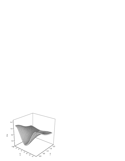
Figure 5: $\hat{E}=Re(\hat{E}_{z})$ as a function of $\hat{z}$ and $\hat{r}$. Here $q=1$, $n=0$ and the first five eigenfunctions have been used. A parabolic transverse profile proportional to $1-k_{1}^{2}\hat{r}^{2}$ with $k_{1}=1.0$ has been used.

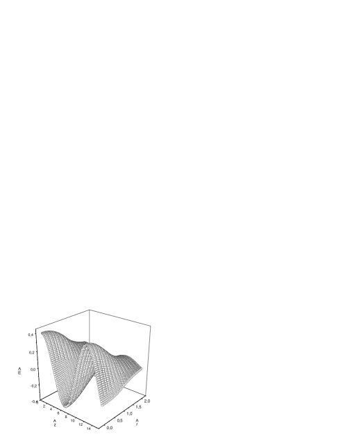
Figure 6: $\hat{E}=Re(\hat{E}_{z})$ as a function of $\hat{z}$ and $\hat{r}$. Here $q=1$, $n=0$ and the first five eigenfunctions have been used. A gaussian transverse profile proportional to $e^{-\hat{r}^{2}/(2\sigma^{2})}$ with $\sigma=2.0$ has been used.

Figure 7: Comparison between analytical results (solid line) and numerical methods (circles). $\hat{E}=Re(\hat{E}_{z})$ is plotted as a function of $\hat{r}$ for several values of $\hat{z}$. Here $q=1$, $n=0$ and the first five eigenfunctions have been used. A stepped transverse profile has been used.

Figure 8: Comparison between analytical results (solid line), multilayer approximation with 15 layers (dotted line) and numerical methods (circles). $\hat{E}=Re(\hat{E}_{z})$ is plotted as a function of $\hat{r}$ for several values of $\hat{z}$. Here $q=1$, $n=0$ and the first five eigenfunctions have been used. A parabolic transverse profile proportional to $1-k_{1}^{2}\hat{r}^{2}$ with $k_{1}=1.0$ has been used.

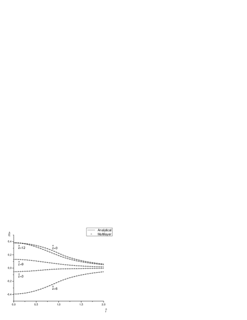
Figure 9: Comparison between multilayer approximation with 15 layers (solid line) and numerical methods (circles). $\hat{E}=Re(\hat{E}_{z})$ is plotted as a function of $\hat{r}$ for several values of $\hat{z}$. Here $q=1$, $n=0$ and the first five eigenfunctions have been used. A gaussian transverse profile proportional to $e^{-\hat{r}^{2}/(2\sigma^{2})}$ with $\sigma=2.0$ has been used.

Eq. (41) can be specialized to the axis-symmetric case by integration of Eq. (38) over the azimuthal angle $\phi$ which leads to

$$\hat{E}_{z}=-iq^{2}\int_{0}^{1}d\hat{r}^{\prime}\left[\hat{r}^{\prime}\sum_{n=-\infty}^{\infty}\hat{j}_{1}^{(n)}G^{(n)}e^{-in\phi}\right]~{},$$ (126)

where

$$G^{(n)}(\hat{r},\hat{r}^{\prime})=\left\{\begin{array}[]{c}I_{n}(q\hat{r})K_{n}(q\hat{r}^{\prime})~{}~{}~{}~{}\hat{r}<\hat{r}^{\prime}\\ I_{n}(q\hat{r}^{\prime})K_{n}(q\hat{r})~{}~{}~{}~{}\hat{r}>\hat{r}^{\prime}\end{array}\right.~{},$$ (127)

$I_{n}$ being the modified Bessel functions of the first kind of order $n$. The equation for the $n$-th azimuthal harmonic of the field can be written from Eq. (126) as

$$\hat{E}_{z}^{(n)}=-iq^{2}\int_{0}^{1}d\hat{r}^{\prime}\hat{r}^{\prime}\hat{j}_{1}^{(n)}G^{(n)}~{}.$$ (128)

Therefore, under the assumption of a cold beam, Eq. (41) can be rewritten as

$$\hat{j}_{1}^{(n)}=\hat{a}_{1d}^{(n)}+i\hat{z}\hat{a}_{1e}^{(n)}$$ (129)

$$+q^{2}S_{0}\int_{0}^{\hat{z}}d\hat{z}\left[(\hat{z}^{\prime}-\hat{z})\int_{0}^{1}d\hat{r}^{\prime}\hat{r}^{\prime}\hat{j}_{1}^{(n)}G^{(n)}\right]~{},$$ (130)

which can be easily transformed, by double differentiation with respect to $\hat{z}$ into the integro-differential equation:

$${d^{2}\hat{j}_{1}^{(n)}\over{d\hat{z}^{2}}}=-q^{2}S_{0}\int_{0}^{1}d\hat{r}^{\prime}\hat{r}^{\prime}G^{(n)}\hat{j}_{1}^{(n)}~{}.$$ (131)

Eq. (131) is of course to be considered together with proper initial conditions for $\hat{j}_{1}$ and its z-derivative at $z=0$. The interval $(0,1)$ can be then divided into an arbitrary number of parts so that Eq. (131) is transformed in a system of the same number of 2nd order coupled differential equations. The possibility of transforming Eq. (131) in a system of 2nd order coupled differential equations explains the choice of starting, in this case, with Eq.(41) instead of Eq. (37): in this way our system can be solved straightforwardly by means of numerical techniques. To do so we used a $4th$-order Runge-Kutta integration method, which gave us the solution of the evolution problem in terms of the beam current. Then, using Eq. (128) we could get back $\hat{E}_{z}$ and we compared obtained results with Eq. (75) for different choices of transverse profiles. The real field $E_{z}$ should be recovered, for any particular situation, passing to the dimensional quantity $\tilde{E}_{z}$ and, then, remembering $E_{z}=\tilde{E}_{z}e^{i\psi}+\tilde{E}^{*}_{z}e^{-i\psi}$: yet, all relevant information is included in $Re(\hat{E}_{z})$. To give first a general idea of the obtained result we present, in Figs. 4, 5 and 6, $Re(\hat{E}_{z})$ as a function of $\hat{z}$ and $\hat{r}$ in the case of stepped, gaussian and parabolic profile respectively, with parameters choice specified in the figure captions. In all cases the initial conditions are proportional to the transverse distribution functions (stepped, gaussian, parabolic), $\hat{F}(\hat{P})=\delta(\hat{P})$ and $n=0$. We consider only initial density modulation (i.e. $\hat{a}_{1e}=0$). Note that, in order to be consistent with the perturbation theory approach we should really choose $\hat{a}_{1d}\ll 1$, since it is normalized to the bunch current density. However using, for example, $\hat{a}_{1d}=\rho$ with $\rho\ll 1$ will simply multiply our results by an inessential factor $\rho$ so, for simplicity, we chose $\rho=1$. Note the oscillatory behavior in the $\hat{z}$ direction. Comparison with the Runge-Kutta integration program are shown in Figs. 7, 8 and 9. In the parabolic case, both pure analytical solution and solution with multilayer approximation method are present, while in the gaussian case only a solution with the multilayer method is possible, to be compared with the numerical Runge-Kutta result. This comparison shows that the assumption of the validity of Eq. (62) is correct in the parabolic case, and validates it once more for the stepped profile situation.

IV.2 The role of the initial condition

Here we present some further exemplification of the obtained results.

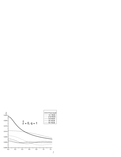
Figure 10: The final result and the first five modes $\hat{a}_{1d}=e^{-\hat{r}^{2}/(2\sigma)}$ with $\sigma=0.1$ at $\hat{z}=0$ and for $q=1$. The final result is the sum of the first fifty modes, here.

Figure 11: The final result and the first five modes $\hat{a}_{1d}=e^{-\hat{r}^{2}/(2\sigma)}$ with $\sigma=0.1$ at $\hat{z}=10$ and for $q=1$. The final result is the sum of the first fifty modes, here.

In particular we are interested in investigating, in a few cases, what is the role of the initial condition in the final results, in order to develop some common sense regarding our analytical formulas.

The main parameter in our system is the transverse beam extent $q$. However, intuitively, one can set two limiting initial conditions: one in which only a small part of the transverse section of the beam is modulated and the other in which all of it is modulated. Depending on the profile of the initial modulation, one can have excitation of many modes or only a few, while the conditions for excitation of a single mode have been discussed in Section III. The transverse parameter $q$ will fix the eigenvalue problem and, therefore, the oscillation wavelength (in the $z$ direction) of the various modes. If $q$ is smaller than or comparable to unity we expect to have appreciable differences in the eigenvalues, which lead to a quick (in $\hat{z}$) change of the relative phases between different modes. As a result the initial shape of the fields will change pretty soon. On the other hand, when $q$ is larger than unity, we will have all the eigenvalues converging to unity as in the one-dimensional case, which means that the relative phases between different modes will stay fixed for a much longer interval in $\hat{z}$ and the initial shape of the fields will not change during the evolution.

Figure 12: The final result and the first five modes $\hat{a}_{1d}=e^{-\hat{r}^{2}/(2\sigma)}$ with $\sigma=0.1$ at $\hat{z}=0$ and for $q=100$. The final result is the sum of the first fifty modes. Here $n=0$.

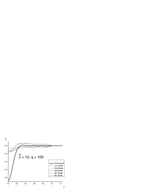
Figure 13: The final result and the first five modes $\hat{a}_{1d}=e^{-\hat{r}^{2}/(2\sigma)}$ with $\sigma=0.1$ at $\hat{z}=10$ and for $q=100$. The final result is the sum of the first fifty modes. Here $n=0$.

To exemplify this situation we set up several calculations using our analytical solutions to the initial value problem. In particular we considered two cases $q=1$ and $q=100$, and a radial stepped profile. Again, we consider only initial density modulation (i.e. $\hat{a}_{1e}=0$) and we study two subcases: in the first we set $\hat{a}_{1d}=e^{-\hat{r}^{2}/(2\sigma)}$ with $\sigma=0.1$ and in the second we put $\hat{a}_{1d}=1$. As said before, in order to be consistent with the perturbation theory approach we should really choose $\hat{a}_{1d}\ll 1$, since it is normalized to the bunch current density but using, for example, $\hat{a}_{1d}=\rho$ with $\rho\ll 1$ will simply multiply our results by an inessential factor $\rho$ so, for simplicity, we chose, again, $\rho=1$. Moreover we considered the azimuthal harmonic $n=0$.

Figures 10 and 11 present the first five eigenfunctions (with relative weights and phases) and the sum of the first fifty (i.e. the final result) for $\hat{a}_{1d}=e^{-\hat{r}^{2}/(2\sigma)}$ with $\sigma=0.1$ at $\hat{z}=0$ and at $\hat{z}=10$ and for $q=1$. As one can see, the relative phases have changed and the shape of the total field, our final result, has also changed with $\hat{z}$.

Figure 14: The final result and the first five modes $\hat{a}_{1d}=1$ at $\hat{z}=0$ and for $q=1$. The final result is the sum of the first fifty modes. Here $n=0$.

Figure 15: The final result and the first five modes $\hat{a}_{1d}=1$ at $\hat{z}=10$ and for $q=100$. The final result is the sum of the first fifty modes. Here $n=0$.

Figure 16: The final result and the first five modes $\hat{a}_{1d}=1$ at $\hat{z}=0$ and for $q=100$. The final result is the sum of the first fifty modes. Here $n=0$.

Figure 17: The final result and the first five modes $\hat{a}_{1d}=1$ at $\hat{z}=10$ and for $q=100$. The final result is the sum of the first fifty modes. Here $n=0$.

On the contrary, Figs. 12 and 13 present the first five eigenfunctions (with relative weights and phases) and the sum of the first fifty (i.e. the final result) for $\hat{a}_{1d}=e^{-\hat{r}^{2}/(2\sigma)}$ with $\sigma=0.1$ at $\hat{z}=0$ and at $\hat{z}=10$, and for $q=100$. Here the relative phases have almost not changed and the shape of the total field, our final result, is also remained unvaried (of course one must account for the fact that the system is undergoing plasma oscillation, so the shape, and not the field magnitude, is what is important here).

Figure 18: The final result and the first five modes when the initial condition is set in order to excite the third mode alone. The final result is the sum of the first fifty modes. Here $n=0$.

Figure 19: The final result and the first five modes when the initial condition is set in order to excite the third mode alone. The final result is the sum of the first fifty modes. Here $n=0$.

For comparison, it is interesting to plot analogous figures for the second situation, that is $\hat{a}_{1d}=1$. Figs. 14 and 15 depict the situation for $q=1$ at $\hat{z}=0$ and $\hat{z}=10$ respectively. The way the phases behave is similar to what has been seen before, i.e. there is a rapid change in the relative phases between the modes, but now it is more difficult to see from the plots because, in contrast with the case of $\hat{a}_{1d}=e^{-\hat{r}^{2}/(2\sigma)}$ already the first mode is sufficient to fit the initial conditions relatively well so that the field shape is almost unchanged. In Figs. 16 and 17 we plot, instead, the case $q=100$ always as $\hat{z}=0$ and $\hat{z}=10$ respectively, and with $\hat{a}_{1d}=1$. Here it is easy to see, once more, that the relative phases between different modes are almost unchanged. What is of interest in this latter set of four pictures is the way different modes are working together to satisfy initial conditions, in comparison with the way they mix in the case for $\hat{a}_{1d}=e^{-\hat{r}^{2}/(2\sigma)}$: note, in particular, how the first mode is almost enough to satisfy the initial conditions (Figs. 14 and 15), while in Figs. 10 and 11 it is almost completely suppressed. This should not be a surprise, considering that we may actually select a single mode by fixing appropriate initial conditions as described in Eq. (83) and Eq. (84). For instance, if we fix $\hat{a}_{1e}=0$ and we want to excite only the $j$th mode for a given value of the azimuthal harmonic $n$ in the case $S_{0}=1$, then, according to Eq. (84) and Eq. (102) we must set (modulus a constant factor):

$$\hat{a}_{1d}={\partial^{2}J_{n}(\alpha_{j}\hat{r})\over{\partial\hat{r}^{2}}}+{1\over{\hat{r}}}{\partial J_{n}(\alpha_{j}\hat{r})\over{\partial\hat{r}}}-\left(q^{2}+{n^{2}\over{\hat{r}^{2}}}\right)J_{n}(\alpha_{j}\hat{r})$$ (132)

where $\alpha_{j}$ is defined in Eq. (101). For example if we choose $n=0$ and $j=2$ (third mode) for $q=1$ we obtain the results presented in Fig. 18 at $\hat{z}=0$ and in Fig. 19 at $\hat{z}=10$. As it can be seen by inspection only the third mode is excited and evolves. Our condition Eq. (132) set strictly to zero the contributions of all the modes with $j\neq 2$. Of course, in practice, actual data plotted in the figures show finite contributions of the other modes ascribed to the finite accuracy of our computations: to be precise, the difference between the final result (sum of the first fifty modes) and the third mode alone was found to be on the fourth significative digit.

V Conclusions

In this paper paper we presented one of the few self-consistent analytical solutions for a system of charged particles under the action of their own electromagnetic fields. Namely, we considered a relativistic electron beam under the action of space-charge at given initial conditions for energy and density modulation and we developed a fully analytical, three-dimensional theory of plasma oscillations in the direction of the beam motion.

We used the assumption of a small modulation so that we could investigate the system behavior in terms of a linearized Vlasov equation coupled with Maxwell equation, under the assumption that field retardation effects can be neglected. Then we introduced normalized quantities according to similarity techniques and we provided two equivalent presentations for the evolution problem in terms of a integrodifferential equation for the electric field and of a integral equation for the beam current.

The integrodifferential equation for the fields was particularly suited to be solved with the help of Laplace transform techniques: we did so in all generality and we discussed the mathematical difficulties involved in the general treatment, namely the assumption of a well-behaved differential operator allowing eigenmodes expansion of the Green function and the problem of the analytic continuation of the Laplace transform of the field to all the complex plane (isolated singularities excluded), in relation with the application of the Fourier-Mellin integral to antitransform $\bar{E}$. Our considerations led us to restrict our attention to the cold beam case. We specialized the general method to the important cases of stepped and parabolic transverse profiles, which are among the few analytically solvable situations. In particular, the stepped profile case could be used to develop a semi-analytical technique to solve the evolution problem for the field using an arbitrary transverse shape.

We tested our results by discussing the limit for the 1-D theory ($q\rightarrow\infty$). We also developed an algorithm able to solve the evolution problem in terms of the beam currents. The integral equation for the currents could be easily approximated to a system of second order ordinary differential equations which could be solved by means of numerical Runge-Kutta integration method. Once the solution for the current was known we recovered the electric field evolution by integration of the current with a suitable Green function. Numerical and analytical or semi-analytical solutions for the fields were then compared and gave a perfect agreement. In this way we could state that the assumption of the correctness of the eigenmodes expansion for the Green function has been proved, for some particular profiles, by means of numerical crosschecks (in the stepped profile case, by means of alternative analytical techniques too).

Finally we exemplified the role of the initial condition, which we have seen to control the way one ore more modes interact together to give the final result. In particular we have shown how to build up initial conditions in such a way that a single mode is excited and propagates through. We checked our prescription by setting up particular initial conditions and looking at the propagation of various eigenmodes.

In conclusion we proposed, checked and analyzed, both from physical and mathematical viewpoint, a theory of space-charge waves on gradient-profile relativistic electron beams. This work is of fundamental importance, since it is one of the few known analytical solution to evolution problems for systems of particles and fields. In particular, today, it is of great relevance in the physics of FEL and high-brightness linear particle accelerators.

VI Acknowledgements

We thank Reinhard Brinkmann (DESY), Martin Dohlus (DESY), Michele Correggi (SISSA), Klaus Floettman (DESY) and Helmut Mais (DESY) for useful discussions. We thank Jochan Schneider (DESY) and Marnix van der Wiel (TUE) for their interest in this work.

References

- (1) J. Rosenzweig et al. in Proc. of Advanced Accelerator Workshop, Lake Tahoe, 1996
- (2) C. Limborg-Deprey, Z. Huang, J. Welch et al., in Proceedings of EPAC2004, Lucerne, Switzerland, to be published
- (3) M. Dohlus, K. Floettmann, O.S.Kozlov et al., Nucl. Instr. and Meth. A, 2004, in press
- (4) TESLA Technical Design Report, DESY 2001-011, edited by F.Richard et. al., and http://tesla.desy.de/
- (5) The LCLS Design Study Group, LCLS Design Study Report, SLAC reports SLAC- R521, Stanford (1998) and http://www-ssrl.slacstanford.edu/lcls/cdr
- (6) L.-H. Yu, M.Babzien, I. Ben-Zvi et al., Science, 289 (2000)
- (7) J. Feldhaus, M. Koerfer, T. Moeller et al., DESY 03-091, ISSN 0418-9833
- (8) E.L. Saldin, E.A. Schneidmiller and M.V. Yurkov, DESY TESLA-FEL-2003-02 and Nucl. Instr. and Meth A, 2004, in press
- (9) E.L. Saldin, E.A. Schneidmiller and M.V. Yurkov, The Physics of Free Electron Lasers, Springer-Verlag, 2000
- (10) E.L. Saldin, E.A. Schneidmiller and M.V. Yurkov, Physics Reports, 260, 1995 p. 187
- (11) H. Alfven, Phys. Rev. 55, 425 (1939)
- (12) J.D. Lawson, J. Electron. Control 3, 587, (1957)
- (13) C.L. Olson and J.W. Poukey, Phys. Rev. A, 9 2631 (1974)
- (14) E.L. Saldin, E.A. Schneidmiller and M.V. Yurkov, Optics Communications, 186, 2000 Pages 185-209
- (15) Yu. L. Klimontovich, Physics-Uspekhi 40 (1), 1997
- (16) Yu. L. Klimontovich, Statistical Physics, Harwood Academic Publ., New York, 1986
- (17) E.M. Lifshitz and L. P. Pitaevskii, Physical Kinetics, Moscow, Nauka, 1979
- (18) S. Krinsky and L.H. Yu. Phys. Rev. A 35 (1987), p. 3406
- (19) A.E. Siegman, Phys. Rev. A 39 (1989), p. 1253
- (20) Bernard Friedman, Principles and Techniques of Applied Mathematics (Wiley, New York, 1956)
- (21) G. Ecker, Theory of Fully Ionized Plasma, Academic Press, New York, 1972