A high-sensitivity laser-pumped $M_{x}$-magnetometer

Abstract

We discuss the design and performance of a laser-pumped cesium vapor magnetometer in the $M_{x}$-configuration. The device will be employed in the control and stabilization of fluctuating magnetic fields and gradients in a new experiment searching for a permanent electric dipole moment of the neutron. We have determined the intrinsic sensitivity of the device to be 29 fT in a 1 Hz bandwidth, limited by low frequency noise of the laser power. In the shot noise limit the magnetometer can reach a sensitivity of 10 fT in a 1 Hz bandwidth. We have used the device to study the fluctuations of a stable magnetic field in a multi-layer magnetic shield for integration times in the range of 2-100 seconds. The residual fluctuations for times up to a few minutes are traced back to the instability of the power supply used to generate the field.

I Introduction

In many areas of fundamental and applied science the sensitive detection of weak magnetic fields and small field fluctuations is of great importance. In the applied sector this concerns, for instance, non-destructive testing of materials Zhang et al. (1995), geomagnetic and archaeological prospecting Becker (1995), and the expanding field of biomagnetism Andrä and Nowak (1998) (eds.). In the realm of fundamental physics, strong demands on magnetometric sensitivity are placed by modern experiments looking for small violations of discrete symmetries in atoms and elementary particles. For instance, many experiments searching for time-reversal or parity violation rely on the precise monitoring and control of magnetic fields, with the sensitivity of the overall experiment directly related to the ultimate sensitivity and stability of the magnetic field detection. Picotesla or even femtotesla sensitivity requirements for averaging times of seconds to minutes are common in that field.

Our particular interest in this respect lies in the search for a permanent electric dipole moment (EDM) of the neutron. Such a moment violates both time reversal invariance and parity conservation. A finite sized EDM would seriously restrict theoretical models that extend beyond the standard model of particle physics Altarev et al. (1996). Recently our team has joined a collaboration aiming at a new measurement of the permanent EDM of ultra-cold neutrons (UCN) to be produced from the UCN source under construction at Paul-Scherrer-Institute in Switzerland SUN . A neutron EDM spectrometer will be used, in which the neutron spin-flip frequency will be measured by a Ramsey resonance method in UCN storage chambers exposed to a homogenous magnetic field. Each neutron chamber has two compartments in which the neutrons are exposed to a static electric field oriented parallel/antiparallel to the magnetic field. The signature of a finite EDM will be a change of the neutron Larmor frequency that is synchronous with the reversal of the relative orientations of the magnetic and electric fields. Magnetic field instabilities and inhomogeneities may mimic the existence of a finite neutron EDM. The control of such systematic effects is therefore a crucial feature of the EDM experiment. It is planned to use a set of optically pumped cesium vapor magnetometers (OPM), operated in the $M_{x}$ configuration Bloom (1962); Aleksandrov et al. (1995) to perform that control.

Although OPMs pumped by spectral discharge lamps are suited for the task, we have opted for a system of laser pumped OPMs (LsOPM). It was shown previously that the replacement of the lamp in an OPM by a resonant laser can lead to an appreciable gain in magnetometric sensitivity Aleksandrov et al. (1995); Aleksandrov (1990). Laser pumping further offers the advantage that a single light source can be used for the simultaneous operation of several dozens of magnetometer heads. In that spirit we have designed and tested a LsOPM with a geometry compatible with the neutron EDM experiment. In this report we present the design and the performance of the Cs-LsOPM operated in a phase-stabilized mode and discuss a systematic effect specifically related to laser pumping.

II The optically-pumped $M_{x}$ magnetometer

Optically pumped magnetometers can reach extreme sensitivities of a few fT$/\sqrt{\mathrm{Hz}}$ Aleksandrov et al. (1995), comparable to standard SQUID (superconducting quantum interference device) detectors. Recently a low field OPM with a sub-fT resolution was demonstrated Kominis et al. (2003). The use of OPMs for the detection of biomagnetic signals was recently demonstrated by our group Bison et al. (2003a, b).

As a general rule the optimum choice of the OPM depends on the specific demands (sensitivity, accuracy, stability, bandwidth, spatial resolution, dynamic range, etc.) of the magnetometric problem under consideration. In our particular case the main requirements are a highest possible sensitivity and stability for averaging times ranging from seconds up to 1000 seconds in a $2\,\mu\mbox{T}$ field together with geometrical constraints imposed by the neutron EDM experiment.

Optically pumped alkali vapor magnetometers rely on an optical-radio frequency (r.f.) resonance technique and are described, e.g., in Bloom (1962). When an alkali vapor is irradiated with circularly polarized light resonant with the D₁ absorption line (transition from the nS_1/2 ground state to the first nP_1/2 excited state), the sample is optically pumped and becomes spin polarized (magnetized) along the direction of the pumping light. While lamp pumped OPMs simultaneously pump all hyperfine transitions of the D₁ line, the use of a monomode laser in a LsOPM allows one to resolve the individual hyperfine transitions provided that their Doppler width does not exceed the hyperfine splitting in both the excited and the ground states. This is, for example, the case for the D₁ transition of the alkali isotopes ¹³³Cs and ⁸⁷Rb. In that case it is advantageous to set the laser frequency to the $F=I+1/2\,\rightarrow\,F=I-1/2$ transition, which allows one to optically pump the atoms into the two (non-absorbing) dark states $|nS_{1/2};F;M_{F}=F,F-1\rangle$ using $\sigma^{+}$ polarized radiation. A magnetic field $\mathbf{B}_{1}(t)$ oscillating at the frequency $\omega_{\mathrm{rf}}$, which is resonant with the Zeeman splitting of the states, drives population out of the dark states into absorbing states, so that the magnetic resonance transition can be detected via a change of the optical transmission of the vapor. That is the very essence of optically detected magnetic resonance.

In the so-called $M_{x}$ or $45^{\circ}$ configuration the static magnetic field $B_{0}$ to be measured is oriented at 45^∘ with respect to the laser beam, while the oscillating magnetic field $\mathbf{B}_{1}(t)$ is at right angles with respect to $\mathbf{B}_{0}$ (Fig. 1). In classical terms, the Larmor precession of the magnetization around $\mathbf{B}_{0}$ (at the frequency $\omega_{L}$) is driven by the co-rotating component of the $\mathbf{B}_{1}(t)$-field, which imposes a phase on the precessing spins. The projection of the precessing polarization onto the propagation direction of the light beam then leads to an oscillating magnetization component along that axis, and therefore to a periodic modulation of the optical absorption coefficient. The system behaves like a classical oscillator, in which the amplitude and the phase of the response (current from a photodiode detecting the transmitted laser intensity) depend in a resonant way on the frequency of the $B_{1}$ field. From the resonance condition $\omega_{L}=\omega_{\mathrm{rf}}$ the Larmor frequency and hence the magnetic field can be inferred.

When the AC component of the detected optical signal is transmitted to the coils producing the $\mathbf{B}_{1}(t)$ field with a 90^∘ phase shift and an appropriate gain, the system will spontaneously oscillate at the resonance frequency. In that self-oscillating configuration the OPM can in principle follow changes of the magnetic field instantaneously with a bandwidth limited by the Larmor frequency only Bloom (1962).

Here we have used an alternative mode of operation, the so-called phase-stabilized mode. The in-phase amplitude $X$, the quadrature amplitude $Y$ and the phase $\phi$ of the photocurrent with respect to the oscillating magnetic field are given by

$$\mathrm{a)}~{}~{}~{} X(x)~{}= -A\,\frac{x}{x^{2}+1+S}$$ (1)

$$\mathrm{b)}~{}~{}~{} Y(x)~{}= -A\,\frac{1}{x^{2}+1+S}$$ (2)

$$\mathrm{c)}~{}~{}~{} \phi(x)~{}= \arctan x\,,$$ (3)

where $x=(\nu_{L}-\nu_{\mathrm{rf}})/\Delta\nu_{\mathrm{HWHM}}$ is the detuning normalized to the (light-power dependent) half width at half maximum $\Delta\nu_{\mathrm{HWHM}}$ of the resonance. $S$ is a saturation parameter which describes the r.f. power broadening of the line. It is interesting to note that the width of the phase dependence, which is determined by the ratio of the $X(x)$ and $Y(x)$ signals, is independent of $S$, and hence immune to r.f. power broadening. The phase $\phi(x)$ changes from $0^{\circ}$ to $-180^{\circ}$ as $\nu_{\mathrm{rf}}$ is tuned over the Larmor frequency. Near resonance the phase is $-90^{\circ}$ and has a linear dependence on the detuning $\nu_{L}-\nu_{\mathrm{rf}}$. $\phi(x)$ is detected by a phase sensitive amplifier (lock-in detector) whose phase output drives a voltage-controlled oscillator (VCO) which feeds the r.f. coils. The VCO signal, phase shifted by $90^{\circ}$, serves as a reference to the phase detector. This feedback loop thus actively locks the r.f. frequency to the Larmor frequency and the magnetometer tracks magnetic field changes in a phase coherent manner. That mode of operation is a modification of the self-oscillating magnetometer in the sense that the lock-in amplifier, the loop filter (PID), and the VCO represent the components of a tracking filter which shifts the detected signal by $90^{\circ}$ and applies the filtered signal to the r.f. coils. The differences to the self-oscillating scheme are the following: the bandwidth of the phase-stabilized magnetometer is determined by the transmission function of the feedback loop, and the phase shift is always $90^{\circ}$ independent of the Larmor frequency, while in the self-oscillating scheme the phase-shifter has a frequency dependence and is $90^{\circ}$ only for a single Larmor frequency. Note that the tracking filter in a strict sense is not a phase-locked loop (PLL), since there is only one detectable frequency in the system, i.e., $\nu_{\mathrm{rf}}$. A detuning between the r.f. frequency and the Larmor frequency produces a static phase shift, while in a real PLL the detuning between the reference frequency and the frequency which is locked produces a time dependent phase shift.

III Magnetometer hardware

The LsOPM for the n-EDM experiment consists of two parts: a sensor head containing no metallic parts except the r.f. coils, and a base station mounted in a portable 19” rack drawer, which contains the frequency stabilized laser and the photodetector. The laser light is carried from the base station to the sensor head by a 10 m long multimode fiber with a core diameter of $800\,\mu$m. The light transmitted through the cell is carried back to the detection unit by a similar fiber. The sensor head is designed to fit into a tube of 104 mm diameter, coaxial with the $2\,\mu$T field, and has a total length of 242 mm. The main component of the sensor is an evacuated glass cell with a diameter of 7 cm containing a droplet of cesium in a sidearm connected to the main volume. A constriction in the sidearm minimizes the collision rate of vapor atoms with the cesium metal. The probability of spin depolarization due to wall collisions with the inner surface of the glass cell is strongly reduced by a thin layer of paraffin coating the cell walls. The cell was purchased from MAGTECH Ltd., St. Petersburg, Russia. A pair of circular coils (70 mm diameter separated by 52 mm) encloses the cell and produces the oscillating magnetic field $\mathbf{B}_{1}(t)$.

The light driving the magnetometer is produced by a tunable extended-cavity diode laser in Littman configuration (Sacher Lasertechnik GmbH, model TEC500). The laser frequency is actively locked to the 4-3 hyperfine component of the Cs D₁ transition ($\lambda=894\,\mbox{nm}$) in an auxiliary cesium vapor cell by means of the dichroic atomic vapor laser lock (DAVLL) technique Yashchuk et al. (2000). The stabilization to a Doppler-broadened resonance provides a continuous stable operation over several weeks and makes the setup rather insensitive to mechanical shocks.

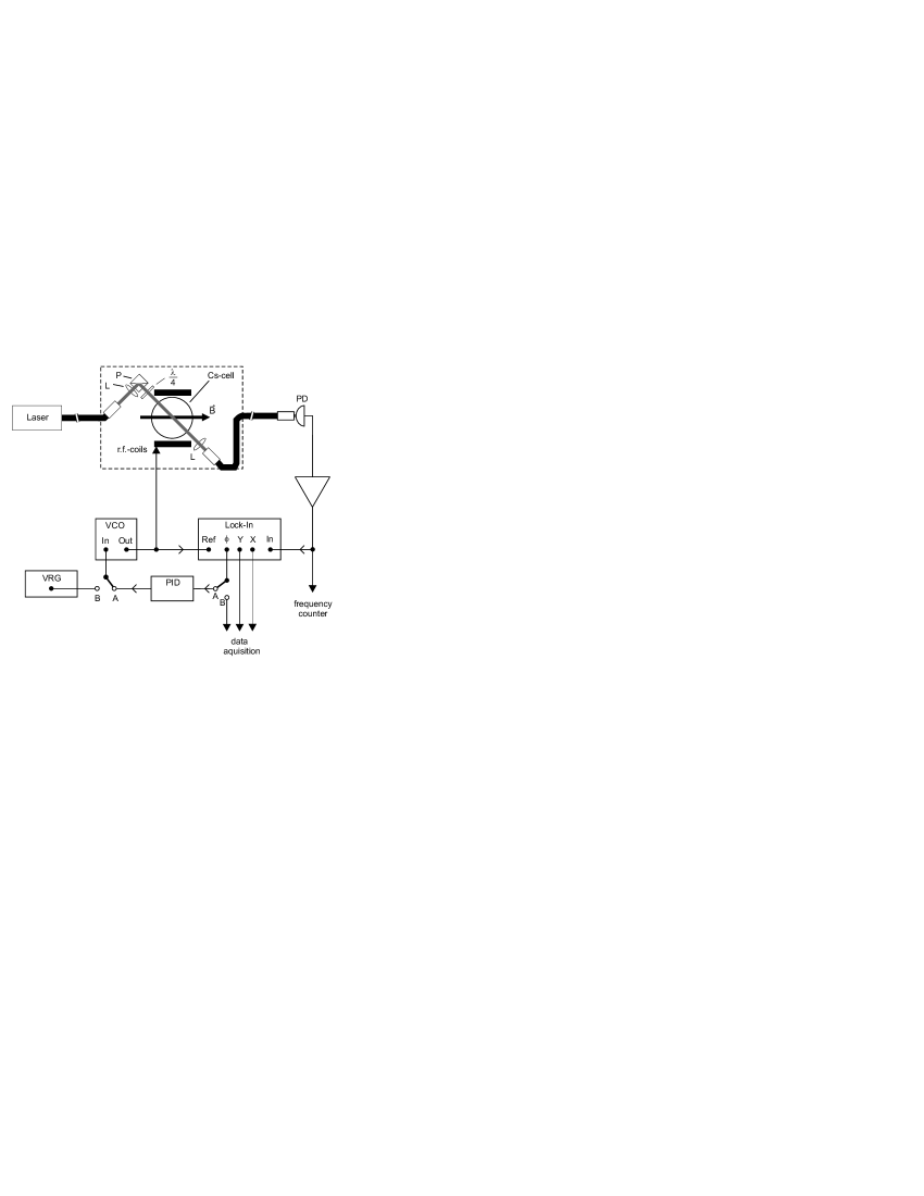
Figure 1: Schematic setup of the phase-stabilized magnetometer in the closed-loop (A) and the scanning (B) mode. The dashed box indicates the sensor head. L: lens, P: polarizing beamsplitter, $\lambda$/4: quarter-wave plate, PD: photodiode, VRG: voltage ramp generator, VCO: voltage-controlled oscillator, PID: feedback amplifier. The stabilization system of the laser frequency is not shown.

At the sensor head the light from the fiber is collimated by a $f=15\,$mm lens and its polarization is made circular by a polarizing beamsplitter and a quarter-wave plate placed before the cesium cell. The light transmitted through the cell is focused into the return fiber, which guides it to a photodiode. The photocurrent is amplified by a low-noise transimpedance amplifier. Placing the laser, the electronics, and the photodiode far away from the sensor head eliminates magnetic interference generated by those components on the magnetometer (a photocurrent of 10 $\mu\mbox{A}$, e.g., produces a magnetic field of 200 pT at a distance of 1 cm). In the present setup the oscillating-field coil is fed via a twisted-pair conductor, which represents an effective antenna by which electromagnetic signals can be coupled into the magnetic shield. In a future stage of development it is planned to replace this electric lead by an opto-coupled system.

Multimode fibers were used for ease of light coupling. We found that a few loops of 3 cm radius of curvature in the fiber led to quasi-depolarization of the initially linearly polarized beam, thereby suppressing noise contributions from polarization fluctuations. A rigid fixation of the fibers was found necessary to reduce power fluctuations of the fiber transmission to a level of $4\times 10^{-5}$ in 1 Hz bandwidth.

The studies reported below were performed inside closed cylindrical shields consisting of three layers of MUMETALL (size of the innermost shield: length 600 mm, diameter 300 mm) that reduces the influence of ambient magnetic field variations. For the measurement of the noise spectrum (Sec. IV.1) and the study of the magnetic field stability (Sec. IV.3) the shield was improved by three additional cylinders of CO-NETIC mounted inside of the MUMETALL shield (innermost diameter 230 mm). The longitudinal bias field of 2 $\mu$T, corresponding to a Cs Larmor frequency of 7 kHz, is produced by a solenoid (length 600 mm, diameter 110 mm) inside the shield and the 8 mA current is provided by a specially designed stable current supply.

III.1 Resonance linewidth

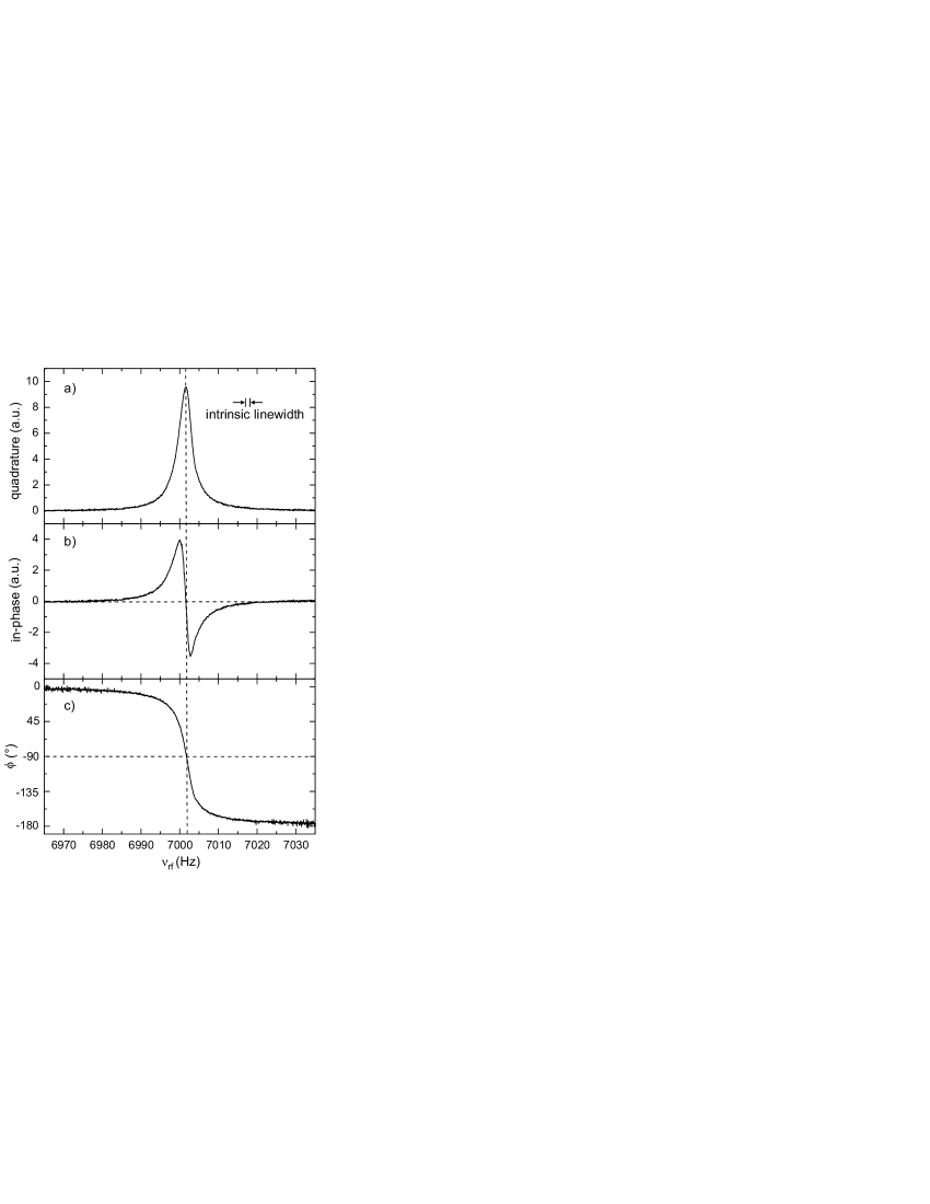
Figure 2: Magnetic resonance spectra obtained by scanning the frequency $\nu_{\mathrm{rf}}$ of the oscillating field: a) quadrature component, b) in-phase component, c) phase between the oscillating field and the modulation of the transmitted power. The Larmor frequency $\nu_{L}$ is 7002.3 Hz, the power-broadened half linewidth is 2.2 Hz. The intrinsic half linewidth of 1.4 Hz is indicated.

The lineshapes of the magnetic resonance line are measured with the magnetometer operating in the open-loop mode (Fig. 1, mode B). A sinusoidally oscillating current of frequency $\omega_{\mathrm{rf}}$ is supplied to the r.f. coils by a function generator, whose frequency is ramped across the Larmor frequency, and the output of the photodiode is demodulated by a lock-in amplifier. Magnetic resonance lines were recorded for different $B_{1}$ amplitudes and different values of the pump light power. Typical resonance lines are shown in Fig. 2. The lineshapes were fitted by the function (3) to the experimental $\phi(\nu_{\mathrm{rf}})$ curves, which allows one to infer the linewidth $\Delta\nu_{\mathrm{HWHM}}$. We recall that the linewidth is not affected by r.f. power broadening, but that it is subject to broadening by the optical pumping process. The dependence of $\Delta\nu_{\mathrm{HWHM}}$ on the laser intensity (Fig. 3) shows that the optical broadening has a nonlinear dependence on the light intensity. The minimum or intrinsic linewidth is determined by extrapolating $\Delta\nu_{\mathrm{HWHM}}$ to zero light intensity.

For a $J=1/2$ two-level system theory predicts a linear dependence of the linewidth on the pumping light intensity, as long as stimulated emission processes from the excited state can be neglected. However, the magnetic resonance spectrum in the $F=4$ manifold of the Cs ground state is a superposition of eight degenerate resonances corresponding to all allowed $\Delta M=\pm 1$ transitions between adjacent Zeeman levels. The coupling of the $\sigma^{+}$ polarized light to the different sublevels depends on their magnetic quantum number $M_{F}$ and is given by the corresponding electric dipole transition matrix elements. As a consequence each of the eight resonances broadens at a different rate. The observed linewidth results from the superposition of those individual lines weighted by the population differences of the levels coupled by the r.f. transition and the corresponding magnetic dipole transition rates. The observed nonlinear dependence of the width on the light intensity follows from the nonlinear way in which those population differences and hence the relative weights are changed by the optical pumping process.

We have calculated the lineshapes of the magnetic resonance lines by numerically solving the Liouville equation for the ground state density matrix. Interactions with the optical field as well as the static and oscillating magnetic fields were taken into account in the rotating wave approximation. We further assumed an isotropic relaxation of the spin coherence at a rate given by the experimentally determined intrinsic linewidth of Fig. 3. The solid curve in that figure represents the linewidths inferred from the calculated lineshapes. The calculations used as a variable an optical pumping rate (proportional to the light power intensity) and the only parameter used to fit the calculation to the experimental data was the proportionality constant between the laser intensity and that pump rate.

The intrinsic linewidth, i.e., the linewidth for vanishing optical and r.f. power, is determined by relaxation due to spin exchange Cs-Cs collisions, Cs-wall collisions, and collisions of the atoms with the Cs droplet in the reservoir sidearm. The latter contribution depends on the ratio of the cross section of the constriction in the sidearm and the inner surface of the spherical cell. With an inner sidearm diameter of 0.5 mm that contribution to the HWHM linewidth can be estimated to be on the order of $\Delta\nu=1$ Hz. The contribution from spin exchange processes at room temperature to the linewidth can be estimated using the cross-section reported in Beverini et al. (1971) to be on the order of 3 Hz, which is larger than the measured width. A possible explanation for this discrepancy is the adsorption of Cs atoms in the paraffin coating Alexandrov et al. (2002), which may lead to an effective vapor pressure in the cell below its thermal equilibrium value.

III.2 Magnetometer mode

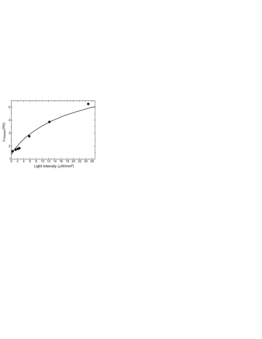
Figure 3: Resonance HWHM linewidth as a function of the light intensity delivered to the cell. The power of the laser beam is given by $I_{L}\cdot 2.8\,\mathrm{mm}^{2}$. The dots represent the widths obtained from the phase signal of the lock-in amplifier with very low r.f. power. The extrapolated intrinsic linewidth is 1.4(1) Hz. The solid line is a one-parameter fit of a numerical calculation to the data (see text). The size of the symbols represents the vertical error bars.

The actual magnetometry is performed in the phase-stabilized mode (Fig. 1, mode A) as described above. The photodiode signal is demodulated by a lock-in amplifier (Stanford Research Systems, model SR830) locked to the driving r.f. frequency, produced by a voltage-controlled oscillator (VCO). The time constant of the lock-in amplifier was set to $\tau=30\,\mu$s, which corresponds to a bandwidth of 2.6 kHz with a $-24$ dB/octave filter roll-off. Either the phase (adjusted to be $0^{\circ}$ on resonance) or the dispersive in-phase signal of the lock-in amplifier can be used to control the VCO, and hence to lock its frequency to the center of the magnetic resonance. Compared to the in-phase signal the phase signal of the lock-in amplifier has the advantage that the resonance linewidth is not affected by r.f. power broadening. However, the bandwidth of the phase output of the digital lock-in amplifier used was limited to 200 Hz by its relatively slow update rate. For the neutron EDM experiment the magnetometer has to be operated with the highest possible bandwidth. We therefore chose the in-phase signal for the following studies. That signal drives the VCO via a feedback amplifier (integrating and differentiating), which closes the feedback loop locking the radio frequency to the Larmor frequency.

IV Performance of the magnetometer

IV.1 Magnetometric sensitivity

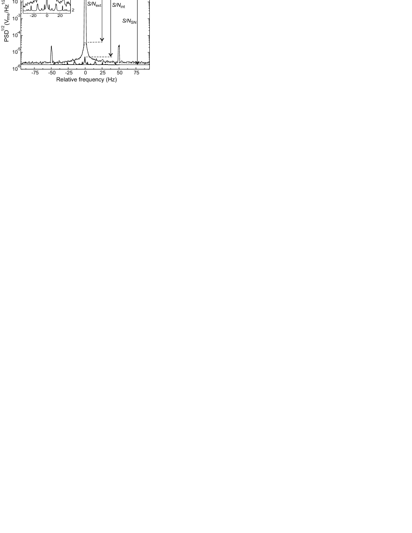
Figure 4: Square root of the power spectral density (PSD) of the magnetometer output frequency relative to the Larmor frequency of $\nu_{0}=6998$ Hz (averaged 20 times). The lowest lying curve is the contribution from laser power noise and $N_{\mathrm{int}}$ its contribution at the Larmor frequency (inset). The straight line indicates the shot noise limit $N_{\mathrm{SN}}$. The signal-to-noise ratio $S/N_{\mathrm{int}}$ is approximately 33000. The sidebands are due to imperfectly shielded magnetic field components oscillating at the 50-Hz power line frequency. The signal-to-noise ratio $S/N_{\mathrm{ext}}$ due to external field fluctuations is approximately 4600. All measurements were performed in a 1 Hz bandwidth.

We characterize the sensitivity of the magnetometer in terms of the noise equivalent magnetic flux density (NEM), which is the flux density change $\delta\!B$ equivalent to the total noise of the detector signal

$$\delta\!B^{2}=\delta\!B_{\mathrm{int}}^{2}+\delta\!B_{\mathrm{ext}}^{2}~{},$$ (4)

with both internal and external contributions: $\delta\!B_{\mathrm{int}}$ describes limitations due to noise sources inherent to the magnetometer proper, while $\delta\!B_{\mathrm{ext}}$ represents magnetic noise due to external field fluctuations. The larger of the two contributions determines the smallest flux density change that the magnetometer can detect. In general the internal NEM $\delta\!B_{\mathrm{int}}$ may have several contributions, which may be expressed as

$$\delta\!B_{\mathrm{int}}^{2}=\left(\frac{1}{\gamma}\times\frac{\Delta\nu_{\mathrm{HWHM}}}{S/N_{\mathrm{SN}}}\right)^{2}+\sum\limits_{i}{\left(\frac{1}{\gamma}\times\frac{\Delta\nu_{\mathrm{HWHM}}}{S/N_{\mathrm{OPM}}^{(i)}}\right)^{2}}~{},$$ (5)

where $S$ is the magnetometer signal, $N_{\mathrm{OPM}}^{(i)}$ are the noise levels of the different processes contributing to $\delta\!B_{\mathrm{int}}$, and $N_{\mathrm{SN}}$ the fundamental shot noise limit of the OPM signal. $\gamma$ is approximately $3.5\,\mbox{Hz/nT}$ for ¹³³Cs and $\Delta\nu_{\mathrm{HWHM}}$ is the half width of the resonance (cf. Sec. IV.2).

The external NEM $\delta\!B_{\mathrm{ext}}$ can be parametrized in the form of Eq. (5) with an equivalent signal noise $N_{\mathrm{ext}}$ so that Eq. (4) can be expressed as

$$\delta\!B=\frac{1}{\gamma}\times\frac{\Delta\nu_{\mathrm{HWHM}}}{S/N},$$ (6)

with $N^{2}=N_{\mathrm{ext}}^{2}+N_{\mathrm{SN}}^{2}+\sum_{i}{\left(N_{\mathrm{OPM}}^{(i)}\right)^{2}}$.

In a strict sense Eqs. (5) and (6) are valid for the open loop operation of the magnetometer. The parameters $\gamma$ and $\Delta\nu_{\mathrm{HWHM}}$ do not depend on the mode of operation, whereas $S/N$ may very well be affected by feedback. If the bandwidth, in which the noise is measured, is much smaller than the loop bandwidth of 1 kHz (cf. Sec. IV.2), it is reasonable to assume that the power spectral density, i.e. $S/N$, is not affected by the loop being opened or closed.

Experimentally the noise levels $N_{\alpha}$ are determined from a Fourier analysis of the photodiode signal, when the magnetometer is operated in the phase-stabilized mode under optimized parameter conditions. Each noise level $N$ is defined as the square root of the integrated (frequency dependent) power spectral density $\rho_{S}^{2}$ of the corresponding signal fluctuations

$$N = \left(\int\limits_{0}^{f_{\mathrm{bw}}}\rho_{S}^{2}\mathrm{d}f\right)^{1/2}~{},$$ (7)

where $f_{\mathrm{bw}}$ is the measurement bandwidth. If the noise is white or if the bandwidth is much smaller than the width of typical spectral features in the power spectrum the noise level at a given frequency $f$ is given by

$$N=\rho_{S}\sqrt{f_{\mathrm{bw}}}=\rho_{S}/\sqrt{2\tau},$$ (8)

where $\tau$ is the integration time used for calculating the Allan standard deviation introduced below. Figure 4 shows a typical Fourier spectrum of the OPM signal. The prominent central feature corresponds to the Larmor oscillation of the photocurrent at 7 kHz during the phase-stabilized operation of the OPM. It is the signal-to-noise ratio at the Larmor frequency which determines the NEM of the magnetometer. The Larmor peak (carrier) is superposed on a 20 Hz broad pedestal, which itself lies above a constant noise floor. The two discrete sidebands originate from magnetic fields oscillating at the 50 Hz line frequency. The pedestal results mainly from imperfectly shielded low-frequency field fluctuations. The continuous spectrum of such fluctuations is mixed with the Larmor frequency and therefore appears as a symmetric background underlying the carrier. We have fitted the pedestal with a Lorentzian lineshape, from which we infer a signal-to-noise ratio $S/N_{\mathrm{ext}}=4600$ at the Larmor frequency, in which $N_{\mathrm{ext}}$ corresponds to magnetic field fluctuations $\delta\!B_{\mathrm{ext}}$ of 210 fT in a 1 Hz bandwidth.

A major contribution to the internal noise $N_{\mathrm{int}}$ comes from laser power fluctuations. This can be understood as follows. The detected photocurrent has the general form $I_{\mathrm{PD}}=I_{\mathrm{pc}}+\Delta I\cos(\omega_{\mathrm{rf}}+\phi)$, where $I_{\mathrm{pc}}$ is the DC component and $\Delta I$ the amplitude of the AC component, which depends on the atomic number density and the degree of spin polarization. If the magnetic resonance signal $\Delta I$ contains fluctuations at frequency $\omega$, these will appear in $I_{\mathrm{PD}}$ at the frequencies $|\omega_{\mathrm{rf}}\pm\omega|$. Low frequency power will therefore produce a symmetric background under the Larmor peak, which also contributes to the pedestal discussed above. In order to distinguish it from the $\delta\!B_{\mathrm{ext}}$ contributions we have measured the low frequency noise spectrum of the laser power. It shows a 1/$f$-like behavior for small frequencies, which levels off at the shot noise value. After mixing with the Larmor frequency its contribution to the magnetometer noise is shown as the lowest lying curve in Fig. 4. The central portion of this spectrum is shown on an expanded scale in the inset. The sidebands are probably due to mechanical vibrations, while the central feature extends $\pm 1.5\,\mbox{Hz}$. $N_{\mathrm{int}}$ represents the contribution of that power noise to the magnetometer noise at the Larmor frequency. The direct contribution to $\delta\!B$ from light power noise is thus negligible compared to the contributions from field fluctuations and confirms the assumption made above that the latter dominate the pedestal. The signal-to-noise ratio $S/N_{\mathrm{int}}$ is 33000 and yields a NEM $\delta\!B_{\mathrm{int}}=29\,\mbox{fT}$ in a 1 Hz bandwidth, determined by laser power fluctuations.

Far away from the Larmor frequency the measured constant noise floor exceeds the calculated shot noise level ($N_{\mathrm{SN}}$) by a factor of 1.5. This may originate from additional noise sources related, e.g., to the laser frequency stabilization. The fundamental limit of the magnetometric sensitivity is determined by the white shot noise $N_{\mathrm{SN}}=\sqrt{2eI_{\mathrm{pc}}f_{\mathrm{bw}}}$ of the DC component of the photocurrent, $I_{\mathrm{pc}}$, which defines the ultimate shot noise limited NEM $\delta\!B_{\mathrm{SN}}$. Under optimized conditions the photocurrent is 5 $\mu$A, which yields a shot noise limited NEM of $\delta\!B_{\mathrm{SN}}=10\,\mbox{fT}$ in a bandwidth of 1 Hz.

Light shift fluctuations are an additional source of noise. Any fluctuations of the parameters causing a light shift (laser power and/or laser frequency detuning) will produce magnetic field equivalent noise. We will show later that for a 1 Hz detection bandwidth this effect gives a negligible contribution to the Fourier spectrum.

As the internal noise level $\delta\!B_{\mathrm{int}}$ is much smaller than the external field fluctuations $\delta\!B_{\mathrm{ext}}$ the magnetometer is well suited to measure the characteristics of such field fluctuations (cf. Sec. IV.3) and/or to compensate them using an active feedback loop. The accuracy of such measurements or the performance of such a stabilization is ultimately limited by the internal noise of the magnetometer, which under ideal conditions can reach the shot noise limit.

IV.2 Magnetometer optimization and response bandwidth

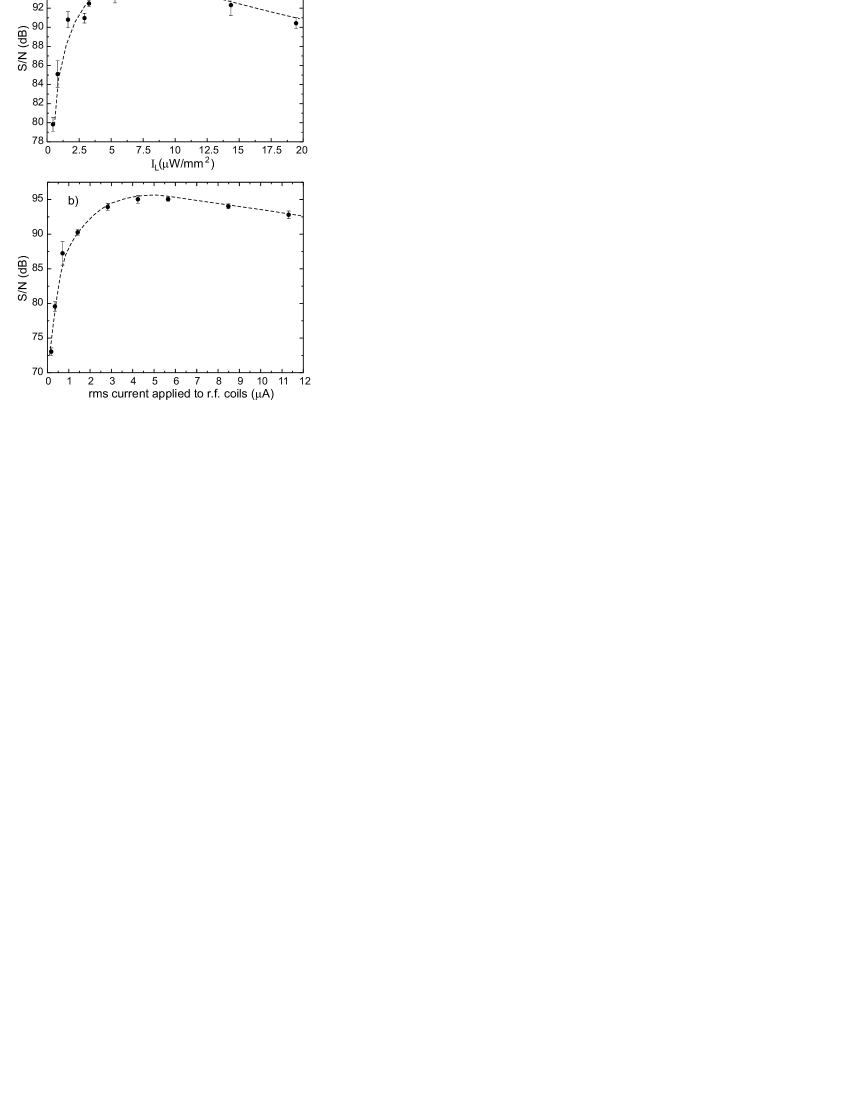
Figure 5: Dependence of the experimental signal-to-noise ratio (measured in a 1 Hz bandwidth) on the light intensity and the current applied to the r.f. coils. The noise was measured 70 Hz away from the carrier. The r.f. current in a) was 8 $\mu$A_pp, the light intensity in b) was 7 $\mu\mathrm{W}/\mathrm{mm}^{2}$. The dashed lines are drawn to guide the eyes. These are typical recordings used to optimize the system parameters.

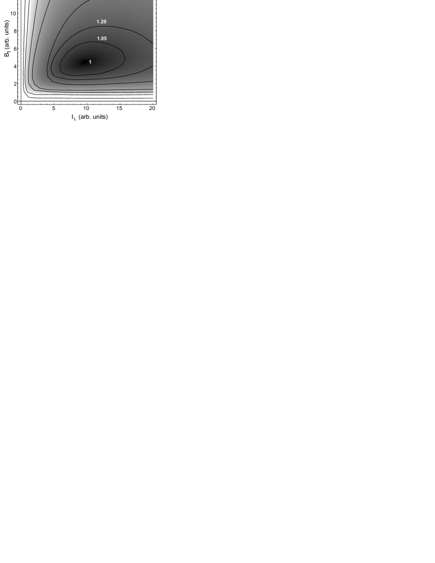
Figure 6: Density plot (in arbitrary units) of the calculated NEM $\delta\!B_{\mathrm{SN}}$, in dependence on the laser intensity $I_{L}$ and the r.f. amplitude $B_{1}$.

According to Eq. (5) the sensitivity of the magnetometer depends on the resonance linewidth $\Delta\nu_{\mathrm{HWHM}}$ and on the signal-to-noise ratio. For given properties of the sensor medium (cesium vapor pressure and cell size) these two properties depend on the two main system parameters, viz., the laser intensity $I_{L}$ (or power $P_{L}$) and the amplitude $B_{1}$ of the r.f. field. For the application in the neutron EDM experiment the sensor size and vapor pressure are dictated by the experimental constraints (fixed geometry and operation at room temperature), so that the experimental optimization of the magnetometric sensitivity is performed in the $\left(I_{L},\,B_{1}\right)$ space by an iterative procedure. Fig. 5 shows examples of signal-to-noise ratio recordings during such an iteration. The optimum operating point was found for a laser intensity $I_{L}$ of $9\,\mu\mbox{W/mm}^{2}$ and a r.f. field amplitude $B_{1}$ of $2.7\,\mbox{nT}$. The resonance linewidth under optimum conditions is $\Delta\nu_{\mathrm{HWHM}}=3.4(1)\,\mbox{Hz}$, which exceeds the intrinsic linewidth by a factor of 2.4.

In order to investigate the dependence of the NEM on the two optimization parameters we have calculated that dependence using the density matrix formalism by assuming that the signal noise is determined by the shot noise of the photocurrent. The result is shown in Fig. 6 as a density plot. One recognizes a broad global minimum which is rather insensitive to the parameter values as it rises only by 5% when the optimum light and r.f. power are varied by 50%.

Figure 7: Frequency dependence of the magnetometer response to a small amplitude sinusoidal modulation of the static field $B_{0}$ (circles). The solid line indicates the amplitude response of a 4^th-order low-pass filter (-24 dB/octave roll-off).

The bandwidth of the magnetometer, i.e., its temporal response to field changes was measured in the following way: a sinusoidal modulation of the static magnetic field with an amplitude of 5 nT was applied by an additional single wire loop (110 mm diameter) wound around the Cs cell. The response of the magnetometer to that perturbation was measured directly on the VCO input voltage in the phase-stabilized mode. The result is shown in Fig. 7. The overall magnetometer response follows the behavior of a low-pass filter ($-24$ dB/octave roll-off) with a -3 dB point at approximately 1 kHz. The lock-in time constant was $30\,\mu\mbox{s}$ which corresponds to a bandwidth of 2.6 kHz. The difference is due to additional filters in the feedback loop.

IV.3 Application: Field fluctuations in a magnetic shield

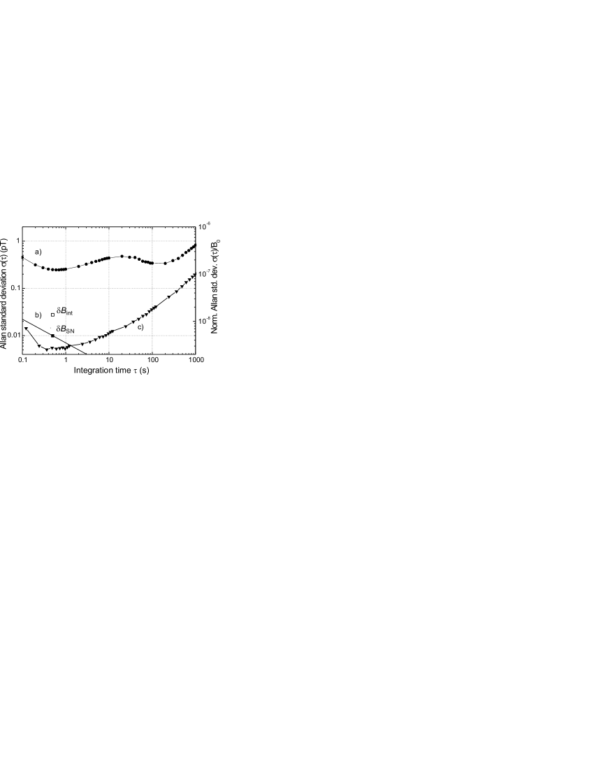
Figure 8: a) Allan standard deviation $\delta\!B_{\mathrm{ext}}$ of the magnetic flux density inside the magnetic shield ($\bullet$). b) NEM $\delta\!B_{\mathrm{int}}$ $(\square)$ limited by laser power fluctuations; extrapolated NEM $\delta\!B_{\mathrm{SN}}~{}(\blacksquare)$ for shot noise limited operation. The slope represents Eq. (8) assuming a white noise behavior. c) Measured contributions to $\delta\!B_{\mathrm{int}}$ from light power fluctuations ($\blacktriangledown$) with present setup. Solid lines in a) and c) are drawn to guide the eye. The dwell time of the frequency counter was 100 ms.

External field fluctuations are the dominant contribution to the noise of the LsOPM when it is operated in the six-layer magnetic shield. We have used the magnetometer to study the temporal characteristics of the residual field variations. The Allan standard deviation Barnes et al. (1971) is the most convenient measure for that characterization. With respect to the experimental specifications of the neutron EDM experiment our particular interest is the field stability for integration times in the range of 100 to 1000 s. For that purpose we recorded the Larmor frequency in multiple time series of several hours with a sampling rate of 0.1 s by feeding the photodiode signal, filtered by a resonant amplifier (band-pass of 200 Hz width centered at 7 kHz), to a frequency counter (Stanford Research Systems, model SR620). From each time series the Allan standard deviation of the flux density inside the shield was calculated. A typical result is shown in Fig. 8 with both absolute and relative scales. For integration times below one second the observed fluctuations (curve a) decrease as $\tau^{-1/2}$, indicating the presence of white field-amplitude noise. It is characterized by a spectral density of 245 fT/$\sqrt{\mbox{Hz}}$. Although the Allan standard deviation represents a different property than the Fourier noise spectrum it is worthwhile to note that the latter value is comparable with the NEM $\delta\!B_{\mathrm{ext}}=210$ fT of the pedestal in Fig. 4 discussed above. The field fluctuations reach a minimum value of approximately 240 fT for an integration time of 0.7 s.

The central region of the Allan plot (Fig. 8a) shows a bump for integration times of 1-100 seconds. It is probably due to fluctuations of the 8 mA current producing the 2 $\mu$T bias field. A magnetic field fluctuation of 200 fT corresponds to a relative current stability of $10^{-7}$, i.e., to current fluctuations of 800 pA. In an auxiliary experiment we measured the current fluctuations $\Delta I$ by recording voltage fluctuations over a series resistor for several hours. We found relative fluctuations of $\Delta I/I$ in the corresponding Allan plot of the same order of magnitude as the $\Delta B/B$ fluctuations. It is thus reasonable to assume that the origin of the plateau in Fig. 8a is due to current fluctuations of the power supply.

The measurement of the magnetic field during several days shows fluctuations with a period of one day and an amplitude of about 1 Hz, superposed by additional uncorrelated drifts. The periodic fluctuations are probably due to changes of the solenoid geometry induced by temperature fluctuations. The Allan standard deviations for integration times exceeding 200 s are thus determined by temperature fluctuations and drifts of the laboratory fields, which are not completely suppressed by the shield.

IV.4 Frequency noise due to light power fluctuations

It is well-known that a near-resonant circularly polarized light field shifts the Zeeman levels in the same way as a static magnetic field oriented along the light beam. The light shift has contributions from the AC Stark shift and coherence shift due to virtual and real transitions Cohen-Tannoudji (1962). The AC Stark shift, and hence the equivalent magnetic field $B_{LS}$ is proportional to the light intensity $I_{L}$ and has a dispersive (Lorentzian) dependence on the detuning of the laser frequency from the center of the optical absorption line. It is therefore expected to vanish at the (optical) line center. In our experiment the laser frequency is locked to the center of a Doppler-broadened hyperfine component. However, that frequency does not coincide with the frequency for which the light shift vanishes, because of finite light shift contributions from the adjacent hyperfine component. While the two hyperfine components are well separated in the optical absorption spectra, their corresponding light shift spectra overlap because of the broad wings of their dispersive lineshapes.

In order to measure the light shift effect we periodically changed the light power between $P+\Delta P/2$ and $P-\Delta P/2$ and recorded the corresponding Larmor frequencies. False effects from drifts of the external magnetic field were suppressed by recording data over several modulation periods. For each modulation amplitude $\Delta P$ the Larmor frequency was measured with both $\sigma^{+}$ and $\sigma^{-}$ polarizations by rotating the quarter-wave plate by means of a mechanical remote control from outside the shield.

The induced changes of the magnetometer readings for both polarizations are shown in Fig. 9. As anticipated, the shift of the Larmor frequency is proportional to the modulation amplitude of the light power and changes sign upon reversing the light helicity. However, it can be seen that the slope of the light shift depends on the helicity. This asymmetry is the result of contributions from three distinct effects, which we discuss only qualitatively here.

(1) The light shift due to virtual transitions (AC Stark shift), which is proportional to the helicity of the light and thus leads to a symmetric contribution to the curves of Fig. 9 (equal in magnitude, but opposite in sign); (2) the light shift due to real transitions (coherence shift)Cohen-Tannoudji (1962), whose origin is a change of the effective $g$-factor of the Cs atom due to the fact that with increasing laser power the atom spends an increasing fraction of its time in the excited state with a 3 times smaller $g_{F}$-factor of opposite sign than that of the ground state; (3) a possible power dependent change of the capacity of the photodiode and a subsequent power dependent phase shift of the photocurrent. The latter two effects yield shifts which have the same sign for both light polarizations, so that the combined contribution of the three effects may explain the different magnitudes of the slopes. A quantitative study of those effects is underway.

Using curve (a) as a worst-case estimate for the fluctuations of the Larmor frequency due to light power fluctuations we estimated, based on measured power fluctuations, the resulting magnetic field fluctuations. The results are shown as triangles in Fig. 8. Light shift fluctuations of the magnetometer readings are thus one to two orders of magnitude smaller than residual field fluctuations in the present shield. The light shift noise can of course be further suppressed by adjusting the laser frequency to the zero light shift frequency point or better by actively stabilizing it to that point or by actively stabilizing the laser power.

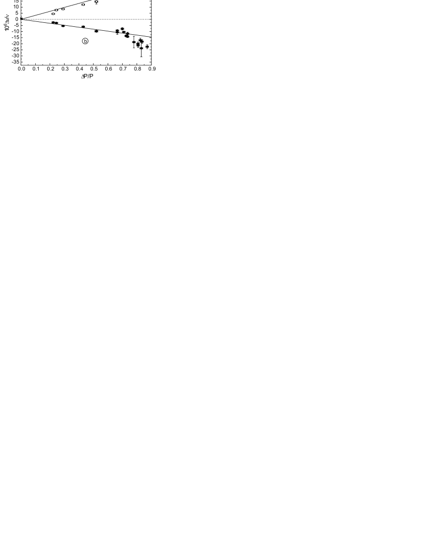
Figure 9: Relative light shift of the Larmor frequency as a function of the relative modulation amplitude $\Delta P$ of the laser power $P$. Curves (a) and (b) represent measurements with light of opposite circular polarization.

V Summary and conclusion

We have described the design and performance of a phase-stabilized cesium vapor magnetometer. The magnetometer has an intrinsic NEM of 29 fT, defined as the Allan standard deviation for an bandwidth of 1 Hz. If the 1/$f$ noise of the laser power can be lowered, e.g., by an active power stabilization and the excess white noise floor can be reduced to the shot noise level the LsOPM should reach a NEM of 10 fT for a 1 Hz bandwidth. The bandwidth of the phase-stabilized LsOPM is 1 kHz. We have used the LsOPM to measure field fluctuations in a six-layer magnetic shield for integration times between 0.1 and 1000 seconds, whose lowest values were found to be on the order of 200-300 fT. Light shift fluctuations, against which no particular precautions were taken, are one to two orders of magnitude smaller than the residual field fluctuations in the shield.

The LsOPM described here compares very favorably with state-of-the-art lamp-pumped magnetometers. Details on that comparison will be published elsewhere. It will be a valuable tool for fundamental physics experiments. The LsOPM presented above meets the requirements of the neutron-EDM experiment on the relevant time scales in the range of 100 to 1000 seconds.

References

- Zhang et al. (1995) Y. Zhang et al., Applied Superconductivity 3, 367 (1995).
- Becker (1995) H. Becker, Archaeological Prospection 2, 217 (1995).
- Andrä and Nowak (1998) (eds.) W. Andrä and H. Nowak (eds.), Magnetism in Medicine (Wiley-VCH, Berlin, 1998).
- Altarev et al. (1996) I. S. Altarev et al., Physics of Atomic Nuclei 59, 1152 (1996).
- (5) See http://ucn.web.psi.ch/.
- Bloom (1962) A. L. Bloom, Appl. Opt. 1, 61 (1962).
- Aleksandrov et al. (1995) E. B. Aleksandrov et al., Opt. Spectrosc. 78, 325 (1995).
- Aleksandrov (1990) E. B. Aleksandrov, Sov. Phys. Tech. Phys. 35, 371 (1990).
- Kominis et al. (2003) I. K. Kominis, T. W. Kornack, J. C. Allred, and M. V. Romalis, Nature 422, 596 (2003).
- Bison et al. (2003a) G. Bison, R. Wynands, and A. Weis, Appl. Phys. B 76, 325 (2003a).
- Bison et al. (2003b) G. Bison, R. Wynands, and A. Weis, Opt. Expr. 11, 904 (2003b).
- Yashchuk et al. (2000) V. V. Yashchuk, D. Budker, and J. R. Davis, Rev. Sci. Instrum. 71, 341 (2000).
- Beverini et al. (1971) N. Beverini, P. Minguzzi, and F. Strumia, Phys. Rev. A 4, 550 (1971).
- Alexandrov et al. (2002) E. B. Alexandrov et al., Phys. Rev. A 66, 042903 (2002).
- Barnes et al. (1971) J. A. Barnes et al., IEEE Trans. Instrum. Meas. 20, 105 (1971).
- Cohen-Tannoudji (1962) C. Cohen-Tannoudji, Ann. Phys. 7, 423 (1962).