Methods for 3-D vector microcavity problems involving a planar dielectric mirror

Abstract

We develop and demonstrate two numerical methods for solving the class of open cavity problems which involve a curved, cylindrically symmetric conducting mirror facing a planar dielectric stack. Such dome-shaped cavities are useful due to their tight focusing of light onto the flat surface. The first method uses the Bessel wave basis. From this method evolves a two-basis method, which ultimately uses a multipole basis. Each method is developed for both the scalar field and the electromagnetic vector field and explicit “end user” formulas are given. All of these methods characterize the arbitrary dielectric stack mirror entirely by its $2\times 2$ transfer matrices for s- and p-polarization. We explain both theoretical and practical limitations to our method. Non-trivial demonstrations are gi ven, including one of a stack-induced effect (the mixing of near-degenerate Laguerre-Gaussian modes) that may persist arbitrarily far into the paraxial limit. Cavities as large as 50$\lambda$ are treated, far exceeding any vectorial solutions previously reported.

1 Introduction

There is currently considerable interest in the nature of electromagnetic (vector) modes both for free space propagation [1, 2, 3, 4] and in cavity resonators [5]. In particular, recent advances in fabrication technology have given rise to optical cavities which cannot be modeled by effectively two-dimensional, scalar or pseudo-vectorial wave equations [6]. The resulting modes may exhibit non-paraxial structure and nontrivial polarization, but this added complexity also gives rise to desirable effects; an example from free-space optics is the observation of enhanced focusing for radially polarized beams [4]. This effect is shown here to arise in cavities as well, among a rich variety of other modes that depend on the three-dimensional geometry. The main goal of this paper is to present a set of numerical techniques adapted to a realistic cavity design as described below.

Much work involving optical cavity resonators utilizes mirrors that are composed of thin layers of dielectric material. These dielectric stack mirrors offer both high reflectivity and a low ratio of loss to transmission, which are desirable in many applications. The simplest model of such cavities treats the mirrors as perfect conductors ($\bm{E}_{\text{tangential}}=\bm{0},H_{\text{normal}}=0$). In applications involving paraxial modes and highly reflective mirrors, it is often acceptable to use this treatment. The mature theory of Gaussian modes (c.f. ​Siegman [7]) is applicable for this class of cavity resonator. When an application requires going beyond the paraxial approximation to describe the optical modes of interest, the problem becomes significantly more involved and modeling dielectric stack mirrors as conducting mirrors may become a poor approximation. Also, one is often interested in the field inside the dielectric stack and for this reason must include the stack structure into the problem.

In this paper we present a group of improved methods for resonators with a cylindrically symmetric curved mirror facing a planar mirror. The paraxial condition is not necessary for these methods; tightly focused modes can be studied. Furthermore, the true vector electromagnetic field is used, rather than a scalar field approximation. The planar mirror is treated as infinite and is characterized by its polarization-dependent reflection functions $r_{s}(\theta_{\text{inc}})$ and $r_{p}(\theta_{\text{inc}})$ for plane waves with incident angle $\theta_{\text{inc}}$. Our model encompasses both cavities for which the planar mirror is an arbitrary dielectric stack, and cavities for which the planar mirror is a simple mirror (conducting with $r_{s/p}(\theta_{\text{inc}})=-1$ or “free” with $r_{s/p}(\theta_{\text{inc}})=+1$). The opposing curved mirror is always treated as a conductor. It should be noted that, for most modes which are highly focused at the planar mirror, (modes which are likely to be of interest in applications), this limitation can be expected to cause little error because the local wave fronts at the curved mirror are mostly perpendicular to its surface. (Of course, for applications in which the curved mirror is indeed conducting, our model is very well suited.) On the other hand, the correct treatment of the planar mirror can be a great improvement over the simplest model. Applications with both dielectric and conducting curved mirrors have been and are currently being used experimentally [5, 8, 9].

The methods described here belong to a class of methods which we refer to as “basis expansion methods”. In basis expansion methods, a complete, orthogonal basis (such as the basis of electromagnetic plane waves) is chosen. Each basis function itself obeys Maxwell’s equations. The equations that determine the correct value of the basis coefficients are boundary equations, resulting from matching appropriate fields at dielectric interfaces, setting appropriate field components to zero at conductor-dielectric interfaces, and setting certain fields to be zero at the origin or infinity. In the usual application of this method, each homogenous dielectric region is allocated its own set of basis coefficients. Our methods use a single set of basis coefficients; the matching between dielectric layers is handled by the $2\times 2$ transfer matrices of the stack.

As dielectric stacks have nonzero transmission, optical cavities with this type of mirror are necessarily open, or lossy. The methods described here deal with the openness due to the stack and the solutions are quasimodes, with discrete, isolated complex wavenumbers which denote both the optimal driving frequency and the resonance width. While the dielectric mirror is partially responsible for the openness of our model system, the openness is not primarily responsible for mode pattern changes resulting from replacing a dielectric stack mirror with a simple mirror. The phase shifts of plane waves reflected off a dielectric stack can vary with incident angle, and it is this variation which can cause significant changes in the modes, even though reflectivities may be greater than $0.99$. Generally speaking, the deviation of $|r_{s/p}(\theta_{\text{inc}})|$ from 1 is not as important as the deviation of $\arg(r_{s/p}(\theta_{\text{inc}}))$ from, say, $\arg(r_{s/p}(0))$.

We develop two general methods, the two-basis method and the Bessel wave method. The scalar field versions of both methods are also developed and are discussed first, acting as pedagogical stepping stones to the vector field versions. The Bessel wave method uses the Bessel wave basis which is the cylindrically symmetric version of the plane wave basis. This method is described in Section 3. The two-basis method ultimately uses the vector or scalar multipole basis. The multipole basis has an advantage in that it is the eigenbasis of a conducting hemisphere, the “canonical” dome-shaped cavity. The unusual aspect of the two-basis method is the intermediate use of the Bessel wave basis. The two-basis method is developed in Section 4. We have implemented both methods and have used them as numerical checks against each other. Various demonstrations and comparisons are given in Section 5. Our implementations of all methods are programmed in C++, use the GSL, LAPACK, SLATEC, and PGPlot numerical libraries, and run on a Macintosh G4 with OS X. Limitations of our model and methods are discussed in Appendix A. Appendix B discusses plotting modes that are associated with linear polarization and Appendix C specifies dielectric stacks that are used in Section 5.

2 Overview of the Model and Notation

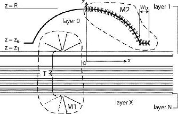
Figure 1: The cavity model.

A diagram of the model is shown in Figure 1. The conducting surface is indicated by the heavy line. The annular portion of this surface extending horizontally from the dome edge will be referred to as the “hat brim”. The dome is cylindrically symmetric with maximum height $z=R$ and edge height $z=z_{e}$. The shape of the dome is arbitrary, but in our demonstrations the dome will be a part of an origin-centered sphere of radius $R_{s}=R$ unless otherwise specified. The region surrounding the curved mirror will be referred to as layer $0$. The dielectric interface between layer $0$ and layer $1$ has height $z=z_{1}$. The last layer of the dielectric stack is layer $N$ and the exit layer is called layer $X$. The depiction of the stack layers in the figure suggests a design in which the stack consists of some layers of experimental interest (perhaps containing quantum wells, dots, or other structures [5, 8]) at the top of the stack where the field intensity is high, and a highly reflective periodic structure below.

At the heart of the procedure to solve for the quasimodes is an overdetermined, complex linear system of equations, $A\bm{y}=\bm{b}$. The column vector $\bm{y}$ is made up of the coefficients of eigenmodes in some basis B. The field in layer $0$ is given by expansion in B using these coefficients. For a given wavenumber, $k$, a solution vector $\bm{y}=\bm{y}_{\text{best}}$ can be found so that $|A(k)\,\bm{y}-\bm{b}|^{2}$ is minimized with respect to $\bm{y}$. Dips in the graph of the residual quantity, $\Delta_{r}\equiv|A(k)\,\bm{y}_{\text{best}}-\bm{b}|$, versus $k$ signify the locations of the isolated eigenvalues of $k$ (theoretically $\Delta_{r}$ should become 0 at the eigenvalues). The solution vector $\bm{y}_{\text{best}}(k)$ at one of these eigenvalues describes a quasimode. The system of equations is made up of three parts (as shown below): M1 equations, M2 equations and an arbitrary amplitude or “seed” equation.

$$A\,\bm{y}=\left[\begin{matrix}\left[\begin{matrix}\\ &M1\\ \end{matrix}\right]\\ \left[\begin{matrix}\\ &M2\\ \end{matrix}\right]\\ \left[\begin{matrix}\text{s. eqn.}\end{matrix}\right]\end{matrix}\right]\bm{\cdot}\left[\begin{matrix}\\ \bm{y}\\ \\ \end{matrix}\right]=\left[\begin{matrix}0\\ \vdots\\ \\ \vdots\\ 0\\ 1\end{matrix}\right].$$ (1)

Henceforth M1 refers to the planar mirror and M2 to the curved mirror.

The M1 boundary condition for a plane wave basis is expressed simply in terms of the $2\times 2$ stack transfer matrices $T_{s}(\theta_{\text{inc}})$ and $T_{p}(\theta_{\text{inc}})$, as suggested by the M1 region (enclosed by the dashed line) in Fig. ​1. In the scalar and vector multipole bases, a sort of conversion to plane waves is required as an intermediate step. The dashed $\bm{k}$ vectors in the figure (incoming from the bottom of the stack) represent plane waves that are given zero amplitude, in order to define a quasimode problem rather than a scattering problem. The plane waves denoted by the solid $\bm{k}$ vectors have nonzero amplitude.

The M2 boundary condition is implemented as follows. A number of locations on the curved mirror are chosen (the “X” marks in Fig. ​1). The width of the hat brim is $w_{b}$ as shown. An “infinitesimal” hat brim ($w_{b}\ll\lambda$) is introduced to give the dome a diffractive edge. An “infinite” hat brim can be introduced theoretically and can make the model more easily understandable in certain respects. More about the model in relation to the hat brim is discussed in Appendix A.2. The M2 equations are the equations in basis B setting the appropriate fields at these locations to zero. For a problem not possessing cylindrical symmetry, these locations would be points. The simplification due to this symmetry, however, allows these locations to be entire rings about the $z$ axis, specified by a single parameter such as the $\rho$ coordinate. Finally, the seed equation sets some combination of basis coefficients equal to one and is the only equation with a nonzero value on the right hand side ($\bm{b}$).

The cylindrical symmetry of the boundary conditions allows one to always find solutions which have a $\phi$ dependence of $\exp(\imath m\phi)$, where $m$ is an integer. This in turn leads to a dimensionally reduced version of the plane wave basis called the Bessel wave basis, in which each basis function is a superposition of all the plane waves with the same wavevector polar angle, $\theta_{k}$. The weight function of the superposition is proportional to $\exp(\imath m\phi_{k})$. We will refer to the non-reduced basis as the “simple plane wave basis”. The unadorned phrase “plane wave basis” (PWB; same abbreviation for plural) will refer henceforth to either or both of the Bessel wave and simple plane wave bases. When using the scalar or vector multipole basis (MB; same abbreviation for plural), cylindrical symmetry allows the problem to be solved separately for each quantum number $m$ of interest. The dimensional reduction in this case amounts to the removal of a summation over $m$ in the basis expansion.

The refractive index in region (layer) $q$ is denoted $\tilde{n}_{q}$. Layers are also denoted with an upper subscript in parenthesis: $\bm{E}^{(q)}$ means the electric vector field in layer $q$. Sometimes “fs” is used as a value of $q$, meaning “in free space” (e.g. ​$\tilde{n}_{\text{fs}}$), whether or not any of the layers in the model we are considering actually are free space. We note here that $\tilde{n}_{\text{fs}}=1$ only in “cavity type I” discussed below.

The symbol $k$, where not in a super/subscript and not bold nor having any super/subscripts, always refers to what may be called the “wavenumber in free space”, although it will have an imaginary part if M1 is a dielectric mirror. An imaginary part in wavenumber, refractive index, and/or frequency is often introduced (as it is in this problem) to turn open cavity problems into eigenvalue problems. The definition of $k$ is as follows. Define $-k_{q}^{2}$ as the constant of separation used to separate space and time equations from the wave equation for layer $q$:

$$\nabla^{2}\text{X}^{(q)}=\frac{\tilde{n}_{q}^{2}}{c^{2}}\frac{\partial^{2}\text{X}^{(q)}}{\partial t^{2}}.$$ (2)

Here $\text{X}^{(q)}$ may be a vector or scalar field. In a few steps, the selection of a global monochromatic time dependence $\exp(-\imath\omega t)$ reveals that the ratio $k_{q}/\tilde{n}_{q}$ is independent of $q$. Then $k$ is defined as $k\equiv k_{\text{fs}}$, so that $k_{q}=n_{q}k$ where $n_{q}\equiv\tilde{n}_{q}/\tilde{n}_{\text{fs}}$. In the model, the index ratios $n_{q}$ are assumed to be real. The single plane wave solution to (2) has the form $\text{X}^{(q)}=C^{(q)}e^{\imath\bm{k}^{(q)}\bm{\cdot x}}e^{-\imath\omega t}$ where $C^{(q)}$ is a constant vector or scalar and the complex wave vector $\bm{k}^{(q)}$ is given by $\bm{k}^{(q)}\equiv k_{q}\bm{\Omega}_{k}^{(q)}=kn_{q}\bm{\Omega}_{k}^{(q)}$ with $\bm{\Omega}_{k}^{(q)}$ being the unit direction vector of the plane wave, specified by $\theta_{k}^{(q)}$ and $\phi_{k}$. The generally complex frequency is given by $\omega=ck_{q}/\tilde{n}_{q}$. At a refractive interface, the angle $\theta_{k}^{(q)}$ changes as given by Snell’s law.

To understand the meaning of a complex $k$, it is helpful to realize that the spatial dependence of the quasimodes are identical in the following two physical cavities:

$$\text{I}: \tilde{n}_{\text{fs}} =1,\tilde{n}_{q}=n_{q},$$

$$\text{II}: \tilde{n}_{\text{fs}} =\Upsilon,\tilde{n}_{q}=\Upsilon n_{q},\Upsilon\in\mathbb{C}.$$ (3)

(The shape and size of each dielectric and conducting region are the same for cavities I and II.) Cavity I is composed of of conductors and zero-gain regions of real refractive index. Cavity II is constructed by taking cavity I and multiplying the refractive index of each region, including free space, by an arbitrary complex number $\Upsilon$. The congruence of the spatial quasimodes follows from separating the variables in (2). The values of $k$, $k_{q}$, and $n_{q}$ for a given quasimode are the same in cavities I and II. The frequency in cavity II is $\omega_{\text{II}}=\omega_{\text{I}}/\Upsilon$. If we henceforth consider only the specific cavity II for which $\Upsilon$ = ($1-\imath g$) where $g$ is tuned to be the ratio $(-\text{Im}k/\text{Re}k)$ (for a given quasimode), we see that $\omega_{\text{II}}=c\text{Re}k=\text{Re}\omega_{\text{I}}$. While in cavity I the quasimode decays in time, in cavity II the quasimode is a steady state because the gain exactly offsets the loss. Either of the two cavity types may be imagined to be the case in our treatment. The only difference is the existence of the decay factor $\exp(c\text{Im}(k)t)$ for cavity I. (The inequality $\text{Im}k\leq 0$ always turns up for an eigenvalue problem with conducting and/or dielectric interface boundary conditions.) We note that the relation of $k$ to the free space wavelength (always real) of a plane wave is $k=(1-\imath g)2\pi/\lambda$. The quality factor, $Q$, of the quasimode is $\text{Re}k/(2|\text{Im}k|)=1/(2g)$.

We note that Snell’s law, $\tilde{n}_{q}\sin\theta_{k}^{(q)}=\tilde{n}_{q+1}\sin\theta_{k}^{(q+1)}$, is independent of whether we have a cavity of type I or II because the quantity $(1-\imath g)$, if present, divides out. One of the limitations of our method is the omission of evanescent waves in layer $0$ and in layers where $n_{q}\geq n_{0}$ (see Appendix A.1). Snell’s law may cause $\theta_{k}^{(q)}$ to become complex for layers with index ratios $n_{q}$ less than $n_{0}$. In this case $\sin\theta_{k}^{(q)}>1$ and $\cos\theta_{k}^{(q)}=\imath{\textrm{sgn}}(\cos\theta_{k}^{(0)})[\sin^{2}\theta_{k}^{(q)}-1]^{1/2}$.

In most cases the symbols $\psi$, $\bm{E}$, and $\bm{H}$ stand for complex-valued fields. The time dependence is $\exp(-\imath\omega t)$ and it is usually suppressed. Physical fields are obtained by multiplying by the time dependence and then taking the real part.

Throughout this paper, the common functions denoted by $Y_{lm}$, $P_{l}^{m}$, $P_{l}$, $J_{n}$, $j_{l}$, and $n_{l}$ are defined as they are in the book by Jackson [10].

In the implementation, $c$ and the related constants $\epsilon_{0}$, $\mu_{0}$, and $Z_{0}$ are all unity, and they will usually be dropped in our treatment. We also assume non-magnetic materials so that $\mu_{q}=\mu_{0}=1$.

3 Plane Wave Bases and the Bessel Wave Method

Although this major section describes the Bessel wave method, much of what is discussed here is applicable to the two-basis method with little alteration. The discussion in Section 4 is greatly shortened due to this overlap of concepts and procedures.

3.1 The Field Expansion in the Simple Plane Wave Bases

3.1.1 Scalar basis

A single scalar plane wave in layer $q$ has the form $\psi=C\exp{(\imath\bm{k}^{(q)\ }\bm{\cdot x}-\imath\omega t)}$. For a general monochromatic field, $k$ and $\omega$ are fixed and the field can be expressed (due to the completeness of the scalar PWB) uniquely (due to the orthogonality of the scalar PWB) as a sum over plane waves in different directions. In our treatment however, we omit plane waves in layer $q$ which would only exist as evanescent waves when refracted into layer $0$. The expansion for the field in layer $q$ is

$$\psi^{(q)}(\bm{x})=\int_{0}^{2\pi}\text{d}\phi_{k}\int_{0}^{\pi}\text{d}\theta_{k}^{(0)}\sin(\theta_{k}^{(0)})\tilde{\psi}_{k}^{(q)}e^{\imath\bm{k}^{(q)}\bm{\cdot x}}.$$ (4)

Here the basis expansion coefficients are the $\tilde{\psi}_{k}^{(q)}$ (continuous coefficients in the integral, and discrete coefficients in implementation). The above expansion effectively propagates each plane wave existing in the cavity down (whether forward or backward) into the stack layers, and adds up all of their contributions. In order to express the $\tilde{\psi}_{k}^{(q)}$ in terms of $\tilde{\psi}_{k}^{(0)}$, it is first necessary to separate the coefficients with $k_{z}>0$ from those with $k_{z}<0$ and write the above expansion as

$$\psi^{(q)}= \;\int_{0}^{2\pi}\text{d}\phi_{k}\int_{0}^{\pi/2}\text{d}\alpha_{k}^{(0)}\sin(\alpha_{k}^{(0)})$$

$$\times\left(\tilde{\psi}_{u}^{(q)}e^{\imath\bm{k}_{u}^{(q)}\bm{\cdot x}}+\tilde{\psi}_{d}^{(q)}e^{\imath\bm{k}_{d}^{(q)}\bm{\cdot x}}\right).$$ (5)

The $u$ and $d$ refer to the plane waves going upward or downward, e.i. ​$\tilde{\psi}_{u}^{(q)}$ is the expansion coefficient $\tilde{\psi}_{k}^{(q)}$ for $k_{z}^{(q)}>0$ (or $k_{z}^{(0)}>0$, since ${\textrm{sgn}}(k_{z}^{(q)})={\textrm{sgn}}(k_{z}^{(0)})$) and $\tilde{\psi}_{d}^{(q)}$ takes the place of $\tilde{\psi}_{k}^{(q)}$ for $k_{z}^{(0)}<0$. The wavevector $\bm{k}^{(q)}$ in cylindrical coordinates is $(k_{\rho}^{(q)},k_{\phi}^{(q)},k_{z}^{(q)})$, for which the following relationships hold:

$$k_{\rho}^{(q)} =k_{q}\sin\theta_{k}^{(q)}=kn_{0}\sin\theta_{k}^{(0)}=kn_{0}\sin\alpha_{k}^{(0)}=k_{\rho}^{(0)},$$

$$k_{z}^{(q)} =k_{q}\cos\theta_{k}^{(q)}=kn_{q}{\textrm{sgn}}(\cos\theta_{k}^{(0)})\cos\alpha_{k}^{(q)}$$

$$=kn_{q}{\textrm{sgn}}(\cos\theta_{k}^{(0)})\sqrt{1-\left(\frac{n_{0}}{n_{q}}\sin\alpha_{k}^{(0)}\right)^{2}},$$

$$k_{\phi}^{(q)} =\phi_{k}\text{ (indep. of $q$).}$$ (6)

This leads to

$$\psi^{(q)}= \;\int_{0}^{2\pi}\text{d}\phi_{k}\int_{0}^{\pi/2}\text{d}\alpha_{k}^{(0)}\sin(\alpha_{k}^{(0)})e^{\imath\varphi_{\rho}}$$

$$\times\left(\tilde{\psi}_{u}^{(q)}e^{\imath\varphi_{z}}+\tilde{\psi}_{d}^{(q)}e^{-\imath\varphi_{z}}\right),$$ (7)

where

$$\varphi_{\rho} \equiv\rho kn_{0}\sin(\alpha_{k}^{(0)})\cos(\phi-\phi_{k}),$$

$$\varphi_{z} \equiv zkn_{q}\cos\alpha_{k}^{(q)}.$$ (8)

From standard theory regarding plane waves and layered media[11], one can calculate the $2\,\times\,2$ complex transfer matrix, $T_{s}^{(q)}$, that obeys the following equation

$$\left(\begin{matrix}\tilde{\psi}_{d}^{(q)}e^{-\imath\varphi_{z}}\\ \tilde{\psi}_{u}^{(q)}e^{\imath\varphi_{z}}\end{matrix}\right)=T_{s}^{(q)}\bm{\cdot}\left(\begin{matrix}\tilde{\psi}_{d}^{(0)}\\ \tilde{\psi}_{u}^{(0)}\end{matrix}\right).$$ (9)

Defining the column sums $\,{}_{+}\beta_{s}^{(q)}\equiv T_{s,12}^{(q)}+T_{s,22}^{(q)}$ and $\,{}_{+}\gamma_{s}^{(q)}\equiv T_{s,11}^{(q)}+T_{s,21}^{(q)}$ allows us to write the expansion of the scalar wave in the layers as

$$\psi^{(q)}= \;\int_{0}^{2\pi}\text{d}\phi_{k}\int_{0}^{\pi/2}\text{d}\alpha_{k}^{(0)}\sin(\alpha_{k}^{(0)})$$

$$\times e^{\imath\varphi_{\rho}}\left(\,{}_{+}\beta_{s}^{(q)}\tilde{\psi}_{u}^{(0)}+\,_{+}\gamma_{s}^{(q)}\tilde{\psi}_{d}^{(0)}\right).$$ (10)

The reason for the notation with the subscripts “+” and “s” will become apparent in the vector discussion. The “s” refers to s-polarization.

The variables in the simple PWB for scalar fields are the complex $\tilde{\psi}_{u}^{(0)}$ and $\tilde{\psi}_{d}^{(0)}$ (the superscript will often be dropped). Next we consider the simple PWB for vector fields.

3.1.2 Vector basis

We assume that for our purposes a general monochromatic electromagnetic field can be expressed uniquely as a sum of vector (electromagnetic) plane waves. For every given frequency and wavevector direction $\bm{\Omega}_{k}$ there are two orthogonally polarized plane waves (as opposed to a single plane wave in the scalar case). Instead of a single coefficient $\tilde{\psi}_{k}$ for each spatial direction we need two, $\tilde{S}_{k}$ and $\tilde{P}_{k}$, which we can define as follows. $\tilde{S}_{k}$ is the amplitude of the vector plane wave propagating in direction $\bm{\Omega}_{k}$ which has its electric field polarized in the $x$-$y$ plane ($E_{z}=0$). Thus, this plane wave is an “s-wave” with regard to the planar mirror. $\tilde{P}_{k}$ is the amplitude of the “p-wave”, the vector plane wave in direction $\bm{\Omega}_{k}$ which has its electric field polarized in the plane of incidence ($E_{\phi}=0$). The coefficients $\tilde{S}_{k}$ and $\tilde{P}_{k}$ will be separated into $\tilde{S}_{u}$, $\tilde{S}_{d}$, $\tilde{P}_{u}$, and $\tilde{P}_{d}$.

To specify the polarization of the fields we will use unit vectors denoted by $\bm{\epsilon}$. The unit vector $\bm{\epsilon}_{s,k}^{(q)}$ denotes the direction of the electric field associated with the plane wave with wavevector $\bm{k}^{(q)}$ and s-polarization. We take the direction of the unit vectors to be:

$$\bm{\epsilon}_{s,k}^{(q)} =-\hat{\bm{\phi}}_{k}$$

$$=\hat{\bm{x}}\sin\phi_{k}-\hat{\bm{y}}\cos\phi_{k},$$

$$\bm{\epsilon}_{p,k}^{(q)} =\hat{\bm{\theta}}_{k}^{(q)}{\textrm{sgn}}(\cos\theta_{k}^{(q)})$$

$$=\hat{\bm{\rho}}_{k}{\textrm{sgn}}(\cos\theta_{k}^{(0)})\cos\theta_{k}^{(q)}-\hat{\bm{z}}{\textrm{sgn}}(\cos\theta_{k}^{(0)})\sin\theta_{k}^{(q)}.$$ (11)

In this phase convention (used by Yeh[11]), the projections of the $\bm{\epsilon}_{p,k}^{(q)}$ vectors for the incident and reflected waves onto the $x$-$y$ plane are equal. The other common phase convention has these projections being in opposite directions.

The entire electric and magnetic field can be broken up into two parts: $\bm{E}^{(q)}=\bm{E}_{s}^{(q)}+\bm{E}_{p}^{(q)}$ and $\bm{H}^{(q)}=\bm{H}_{s}^{(q)}+\bm{H}_{p}^{(q)}$ where $\bm{H}_{s}^{(q)}$ is the field with magnetic s-polarization ($H_{z}=0$) and $\bm{H}_{p}^{(q)}$ is the field with magnetic p-polarization ($H_{\phi}=0$). We can now write down the most compact expansion of the vector field.

$$\bm{E}_{s}^{(q)} =\int\textbf{d}\bm{\Omega}_{k}^{(0)}\tilde{S}_{k}^{(q)}\bm{\epsilon}_{s,k}^{(q)}e^{\imath\bm{k}^{(q)}\bm{\cdot x}},$$

$$\bm{E}_{p}^{(q)} =\int\textbf{d}\bm{\Omega}_{k}^{(0)}\tilde{P}_{k}^{(q)}\bm{\epsilon}_{p,k}^{(q)}e^{\imath\bm{k}^{(q)}\bm{\cdot x}},$$

$$\bm{H}_{s}^{(q)} =-\tilde{n}_{q}\int\textbf{d}\bm{\Omega}_{k}^{(0)}\tilde{P}_{k}^{(q)}\bm{\epsilon}_{s,k}^{(q)}{\textrm{sgn}}(\cos\theta_{k}^{(0)})e^{\imath\bm{k}^{(q)}\bm{\cdot x}},$$

$$\bm{H}_{p}^{(q)} =\tilde{n}_{q}\int\textbf{d}\bm{\Omega}_{k}^{(0)}\tilde{S}_{k}^{(q)}\bm{\epsilon}_{p,k}^{(q)}{\textrm{sgn}}(\cos\theta_{k}^{(0)})e^{\imath\bm{k}^{(q)}\bm{\cdot x}}.$$ (12)

The factors of $\tilde{n}_{q}$ in the $H$ equations come from the physical relation of $H$ to $E$ for a plane wave. Note that $\tilde{n}_{q}$ is different for cavity types I and II (as given in Eqn. (3)). Separating up and down coefficients yields

$$\bm{E}_{s}^{(q)}= \;\int_{0}^{2\pi}\text{d}\phi_{k}\,\bm{\epsilon}_{s,k}^{(q)}\int_{0}^{\pi/2}\text{d}\alpha_{k}^{(0)}\sin(\alpha_{k}^{(0)})e^{\imath\varphi_{\rho}}$$

$$\times\left(\tilde{S}_{u}^{(q)}e^{\imath\varphi_{z}}+\tilde{S}_{d}^{(q)}e^{-\imath\varphi_{z}}\right),$$

$$\bm{E}_{p}^{(q)}= \;\int_{0}^{2\pi}\text{d}\phi_{k}\int_{0}^{\pi/2}\text{d}\alpha_{k}^{(0)}\sin(\alpha_{k}^{(0)})\,e^{\imath\varphi_{\rho}}$$

$$\times\Bigl{[}\hat{\bm{\rho}}_{k}\cos(\alpha_{k}^{(q)})\left(\tilde{P}_{u}^{(q)}e^{\imath\varphi_{z}}+\tilde{P}_{d}^{(q)}e^{-\imath\varphi_{z}}\right)$$

$$+\hat{\bm{z}}\sin(\alpha_{k}^{(q)})\left(-\tilde{P}_{u}^{(q)}e^{\imath\varphi_{z}}+\tilde{P}_{d}^{(q)}e^{-\imath\varphi_{z}}\right)\Bigr{]}.$$ (13)

These expressions explicitly use coordinate vectors only where necessary due to a dependence of the $\bm{\epsilon}_{k}$ vectors on the sign of $\cos\theta_{k}^{(0)}$. The expressions for $\bm{H}^{(q)}$ are omitted for brevity.

To relate $\tilde{S}_{u/d}^{(q)}$ and $\tilde{P}_{u/d}^{(q)}$ to $\tilde{S}_{u/d}^{(0)}$ and $\tilde{P}_{u/d}^{(0)}$ we can use the transfer matrices: $T_{s}$ for s-polarized light and $T_{p}$ for p-polarized light. The transfer matrix used for the scalar field in Eqn. (9) is the same matrix we will use here for s-polarization. These matrices perform the following transformations

$$\left(\begin{matrix}\tilde{S}_{d}^{(q)}e^{-\imath\varphi_{z}}\\ \tilde{S}_{u}^{(q)}e^{\imath\varphi_{z}}\end{matrix}\right) =T_{s}^{(q)}\,\bm{\cdot}\,\left(\begin{matrix}\tilde{S}_{d}^{(0)}\\ \tilde{S}_{u}^{(0)}\end{matrix}\right),$$

$$\left(\begin{matrix}\tilde{P}_{d}^{(q)}e^{-\imath\varphi_{z}}\\ \tilde{P}_{u}^{(q)}e^{\imath\varphi_{z}}\end{matrix}\right) =T_{p}^{(q)}\,\bm{\cdot}\,\left(\begin{matrix}\tilde{P}_{d}^{(0)}\\ \tilde{P}_{u}^{(0)}\end{matrix}\right).$$ (14)

We define

$$\,{}_{\pm}\beta_{s}^{(q)} \equiv T_{s,12}^{(q)}\pm T_{s,22}^{(q)},$$

$$\,{}_{\pm}\gamma_{s}^{(q)} \equiv T_{s,21}^{(q)}\pm T_{s,11}^{(q)},$$

$$\,{}_{\pm}\beta_{p}^{(q)} \equiv T_{p,12}^{(q)}\pm T_{p,22}^{(q)},$$

$$\,{}_{\pm}\gamma_{p}^{(q)} \equiv T_{p,21}^{(q)}\pm T_{p,11}^{(q)}.$$ (15)

Note $\,{}_{+}\beta_{s}^{(q)}$ and $\,{}_{+}\gamma_{s}^{(q)}$ are defined as before. The $\beta$ and $\gamma$ quantities are functions of $z$ and $z_{1}$ and not of $\rho$ or $\phi$. They are functions of $k$ and $\alpha_{k}^{(0)}$ but not of $\phi_{k}$.

Now the field expansions become

$$\bm{E}_{s}^{(q)}= \;\int_{0}^{2\pi}\text{d}\phi_{k}\,\bm{\epsilon}_{s,k}^{(q)}\int_{0}^{\pi/2}\text{d}\alpha_{k}^{(0)}\sin(\alpha_{k}^{(0)})e^{\imath\varphi_{\rho}}$$

$$\times\left(\,{}_{+}\beta_{s}^{(q)}\tilde{S}_{u}^{(0)}+\,_{+}\gamma_{s}^{(q)}\tilde{S}_{d}^{(0)}\right),$$

$$\bm{E}_{p}^{(q)}= \;\int_{0}^{2\pi}\text{d}\phi_{k}\int_{0}^{\pi/2}\text{d}\alpha_{k}^{(0)}\sin(\alpha_{k}^{(0)})\,e^{\imath\varphi_{\rho}}$$

$$\times\Bigl{[}\hat{\bm{\rho}}_{k}\cos(\alpha_{k}^{(q)})\left(\,{}_{+}\beta_{p}^{(q)}\tilde{P}_{u}^{(0)}+\,_{+}\gamma_{p}^{(q)}\tilde{P}_{d}^{(0)}\right)$$

$$+\hat{\bm{z}}\sin(\alpha_{k}^{(q)})\left(\,{}_{-}\beta_{p}^{(q)}\tilde{P}_{u}^{(0)}-\,_{-}\gamma_{p}^{(q)}\tilde{P}_{d}^{(0)}\right)\Bigr{]},$$

$$\bm{H}_{s}^{(q)}= \;\tilde{n}_{q}\int_{0}^{2\pi}\text{d}\phi_{k}\,\bm{\epsilon}_{s,k}^{(q)}\int_{0}^{\pi/2}\text{d}\alpha_{k}^{(0)}\sin(\alpha_{k}^{(0)})e^{\imath\varphi_{\rho}}$$

$$\times\left(\,{}_{-}\beta_{p}^{(q)}\tilde{P}_{u}^{(0)}-\,_{-}\gamma_{p}^{(q)}\tilde{P}_{d}^{(0)}\right),$$

$$\bm{H}_{p}^{(q)}= \;\tilde{n}_{q}\int_{0}^{2\pi}\text{d}\phi_{k}\int_{0}^{\pi/2}\text{d}\alpha_{k}^{(0)}\sin(\alpha_{k}^{(0)})\,e^{\imath\varphi_{\rho}}$$

$$\times\Bigl{[}\hat{\bm{\rho}}_{k}\cos(\alpha_{k}^{(q)})\left(-\,_{-}\beta_{s}^{(q)}\tilde{S}_{u}^{(0)}+\,_{-}\gamma_{s}^{(q)}\tilde{S}_{d}^{(0)}\right)$$

$$-\hat{\bm{z}}\sin(\alpha_{k}^{(q)})\left(\,{}_{+}\beta_{s}^{(q)}\tilde{S}_{u}^{(0)}+\,_{+}\gamma_{s}^{(q)}\tilde{S}_{d}^{(0)}\right)\Bigr{]}.$$ (16)

The variables in the simple PWB for vector fields are the complex $\tilde{S}_{u}^{(0)}$, $\tilde{S}_{d}^{(0)}$, $\tilde{P}_{u}^{(0)}$, and $\tilde{P}_{d}^{(0)}$ (the superscript will often be dropped).

3.2 The Field Expansion in the Bessel Wave Bases

3.2.1 Scalar basis

We have already assumed a time dependence of $\exp(-\imath\omega t)$. As mentioned in the Overview, a cylindrically symmetric set of boundary conditions allows us to assume an azimuthal dependence of $\exp(\imath m\phi)$ with $m$ being an integer. Consider the expansion (4). We wish to find the conditions on $\tilde{\psi}_{k}^{(q)}$ which cause the entire dependence of $\psi(\bm{x})$ on $\phi$ to be $\exp(\imath m\phi)$.

The general Fourier series expansion of $\tilde{\psi}_{k}^{(q)}$ is

$$\tilde{\psi}_{k}^{(q)}(\theta_{k}^{(0)},\phi_{k})=\sum_{n}f_{n}^{(q)}(\theta_{k}^{(0)})\,e^{\imath n\phi_{k}}.$$ (17)

We can then write (4) as

$$\psi^{(q)}= \;\sum_{n}\int_{0}^{\pi}\text{d}\theta_{k}^{(0)}\sin(\theta_{k}^{(0)})e^{\imath\tilde{\varphi}_{z}}f_{n}^{(q)}(\theta_{k}^{(0)})$$

$$\times\int_{0}^{2\pi}\,\text{d}\phi_{k}\;e^{\imath\rho kn_{0}\sin(\theta_{k}^{(0)})\cos(\phi-\phi_{k})}e^{\imath n\phi_{k}},$$ (18)

where

$$\tilde{\varphi}_{z}\equiv zkn_{q}\cos\theta_{k}^{(q)}.$$ (19)

The last integral is of the solved form

$$\int_{0}^{2\pi}e^{\imath y\cos(\phi^{{}^{\prime}}-\phi)}e^{\imath n\phi^{{}^{\prime}}}\text{d}\phi^{{}^{\prime}}=2\pi(\imath)^{n}J_{n}(y)e^{\imath n\phi},$$ (20)

where $J_{n}$ denotes the regular Bessel function of order $n$ ($n$ can be negative). This yields

$$\psi^{(q)}= \;2\pi\sum_{n}(\imath)^{n}e^{\imath n\phi}\int_{0}^{\pi}\text{d}\theta_{k}^{(0)}\sin(\theta_{k}^{(0)})$$

$$\times e^{\imath\tilde{\varphi}_{z}}J_{n}(\rho kn_{0}\sin\theta_{k}^{(0)})f_{n}^{(q)}(\theta_{k}^{(0)}).$$ (21)

In order to have only $\exp(\imath m\phi)$ dependence on $\phi$, the integral on the right hand side must be zero for $n\neq m$. Because $f_{n}^{(q)}(\theta_{k}^{(0)})$ cannot be a function of $z$ or $\rho$, the only way to have this for all $z$ and $\rho$ is to pick $f_{n}=0$ for $n\neq m$. Thus $\tilde{\psi}_{k}^{(q)}(\theta_{k}^{(0)},\phi_{k})=f_{m}^{(q)}(\theta_{k}^{(0)})e^{\imath m\phi_{k}}$. At this point we define the symbol $\psi_{k}^{(q)}$ to mean the coefficient $f_{m}^{(q)}$. The cylindrically symmetric expansion is

$$\psi^{(q)}= \;\xi\int_{0}^{\pi}\!\text{d}\theta_{k}^{(0)}\sin(\theta_{k}^{(0)})e^{\imath\tilde{\varphi}_{z}}J_{m}(\rho kn_{0}\sin\theta_{k}^{(0)})\psi_{k}^{(q)}(\theta_{k}^{(0)}),$$ (22)

where

$$\xi\equiv 2\pi(\imath)^{m}e^{\imath m\phi}.$$ (23)

This is an expansion in scalar Bessel waves, defined to be

$$\xi\exp(\imath zkn_{q}\cos\theta_{k}^{(q)})J_{m}(\rho kn_{0}\sin\theta_{k}^{(0)}),$$ (24)

with $\{\psi_{k}^{(q)}(\theta_{k}^{(0)})\}$ being the set of coefficients. Each Bessel wave is a set of simple plane waves with fixed polar angle but having the full range (0 to $2\pi$) of azimuthal angles, $\phi_{k}$. The weight factors of the plane waves are proportional to $\exp(\imath m\phi_{k})$. The final cylindrically symmetric scalar expansion with up and down separated is

$$\psi^{(q)}(\bm{x})= \;\xi\int_{0}^{\pi/2}\text{d}\alpha_{k}^{(0)}\sin(\alpha_{k}^{(0)})J_{m}(\rho kn_{0}\sin\alpha_{k}^{(0)})$$

$$\times\left(\,{}_{+}\beta_{s}^{(q)}\psi_{u}^{(0)}+\,_{+}\gamma_{s}^{(q)}\psi_{d}^{(0)}\right).$$ (25)

The $\psi_{u}^{(0)}$ and $\psi_{d}^{(0)}$ are the (complex) variables in the Bessel wave method for scalar fields; they make up the solution vector $\bm{y}$ in (1).

3.2.2 Vector basis

For cylindrically symmetric boundary conditions, the $\phi$ dependence of $E_{\rho}$, $E_{z}$, $E_{\phi}$, $H_{\rho}$, $H_{z}$, and $H_{\phi}$ can be taken (for a single mode) to be $\exp(\imath m\phi)$.

Consider doing the $\phi_{k}$ integrations in (12) or (16). The unit vectors $\bm{\epsilon}_{s/p,k}^{(q)}$ and $\hat{\bm{\rho}}_{k}$ depend on $\phi_{k}$. The $z$ components do not depend on $\phi_{k}$ so we will look at these first. There is no contribution to the $z$ component of the electric field from $\bm{E}_{s}^{(q)}$ nor is there any contribution to the $z$ component of the magnetic field from $\bm{H}_{s}^{(q)}$. We define

$$\,{}_{z}P^{(q)}(\bm{x}) \equiv\bm{E}^{(q)}\bm{\cdot}\hat{\bm{z}}=\bm{E}_{p}^{(q)}\bm{\cdot}\hat{\bm{z}},$$

$$\,{}_{z}^{H}\!P^{(q)}(\bm{x}) \equiv\bm{H}^{(q)}\bm{\cdot}\hat{\bm{z}}=\bm{H}_{p}^{(q)}\bm{\cdot}\hat{\bm{z}}.$$ (26)

Requiring that these quantities have an $\exp(\imath m\phi)$ dependence produces results similar to the scalar case. Defining

$$S_{k}^{(q)}e^{\imath m\phi_{k}}\equiv\tilde{S}_{k}^{(q)},$$

$$P_{k}^{(q)}e^{\imath m\phi_{k}}\equiv\tilde{P}_{k}^{(q)},$$ (27)

and using (16), we have the final, useful expansions for ${}_{z}P^{(q)}$ and ${}_{z}^{H}\!P^{(q)}$:

$$\,{}_{z}P^{(q)}= \;\xi\int_{0}^{\pi/2}\text{d}\alpha_{k}^{(0)}\sin(\alpha_{k}^{(0)})\sin(\alpha_{k}^{(q)})$$

$$\times J_{m}(\rho kn_{0}\sin\alpha_{k}^{(0)})\left(\,{}_{-}\beta_{p}^{(q)}P_{u}^{(0)}-\,_{-}\gamma_{p}^{(q)}P_{d}^{(0)}\right),$$

$$\,{}_{z}^{H}\!P^{(q)}= \;-\xi\tilde{n}_{q}\int_{0}^{\pi/2}\text{d}\alpha_{k}^{(0)}\sin(\alpha_{k}^{(0)})\sin(\alpha_{k}^{(q)})$$

$$\times J_{m}(\rho kn_{0}\sin\alpha_{k}^{(0)})\left(\,{}_{+}\beta_{s}^{(q)}S_{u}^{(0)}+\,_{+}\gamma_{s}^{(q)}S_{d}^{(0)}\right).$$ (28)

To deal with the transverse part of the electromagnetic field it is helpful to use quantities related to circular polarization. We define

$$\,{}_{\pm}S^{(q)} \equiv\pm\imath\bm{E}_{s}^{(q)}\bm{\cdot}\hat{\bm{x}}-\bm{E}_{s}^{(q)}\bm{\cdot}\hat{\bm{y}}$$

$$=e^{\pm\imath\phi}(\pm\imath\bm{E}_{s}^{(q)}\bm{\cdot}\hat{\bm{\rho}}-\bm{E}_{s}^{(q)}\bm{\cdot}\hat{\bm{\phi}}),$$

$$\,{}_{\pm}^{H}\!S^{(q)} \equiv\pm\imath\bm{H}_{s}^{(q)}\bm{\cdot}\hat{\bm{x}}-\bm{H}_{s}^{(q)}\bm{\cdot}\hat{\bm{y}}$$

$$=e^{\pm\imath\phi}(\pm\imath\bm{H}_{s}^{(q)}\bm{\cdot}\hat{\bm{\rho}}-\bm{H}_{s}^{(q)}\bm{\cdot}\hat{\bm{\phi}}),$$

$$\,{}_{\pm}P^{(q)} \equiv\bm{E}_{p}^{(q)}\bm{\cdot}\hat{\bm{x}}\pm\imath\bm{E}_{p}^{(q)}\bm{\cdot}\hat{\bm{y}}$$

$$=e^{\pm\imath\phi}(\bm{E}_{p}^{(q)}\bm{\cdot}\hat{\bm{\rho}}\pm\imath\bm{E}_{p}^{(q)}\bm{\cdot}\hat{\bm{\phi}}),$$

$$\,{}_{\pm}^{H}\!P^{(q)} \equiv\bm{H}_{p}^{(q)}\bm{\cdot}\hat{\bm{x}}\pm\imath\bm{H}_{p}^{(q)}\bm{\cdot}\hat{\bm{y}}$$

$$=e^{\pm\imath\phi}(\bm{H}_{p}^{(q)}\bm{\cdot}\hat{\bm{\rho}}\pm\imath\bm{H}_{p}^{(q)}\bm{\cdot}\hat{\bm{\phi}}).$$ (29)

Inverting (29) yields

$$\bm{E}_{s}^{(q)}\bm{\cdot}\hat{\bm{\rho}} =\frac{-\imath}{2}(\,_{+}S^{(q)}e^{-\imath\phi}-\,_{-}S^{(q)}e^{\imath\phi}),$$

$$\bm{E}_{s}^{(q)}\bm{\cdot}\hat{\bm{\phi}} =\frac{-1}{2}(\,_{+}S^{(q)}e^{-\imath\phi}+\,_{-}S^{(q)}e^{\imath\phi}),$$

$$\bm{E}_{p}^{(q)}\bm{\cdot}\hat{\bm{\rho}} =\frac{1}{2}(\,_{+}P^{(q)}e^{-\imath\phi}+\,_{-}P^{(q)}e^{\imath\phi}),$$

$$\bm{E}_{p}^{(q)}\bm{\cdot}\hat{\bm{\phi}} =\frac{-\imath}{2}(\,_{+}P^{(q)}e^{-\imath\phi}-\,_{-}P^{(q)}e^{\imath\phi}),$$ (30)

with the magnetic field quantities having similar relations. Now we use (12) and (11) with (29). The resulting electric field quantities are

$$\,{}_{\pm}S^{(q)}= \;\int_{0}^{\pi}\,\text{d}\theta_{k}^{(0)}\sin(\theta_{k}^{(0)})e^{\imath\tilde{\varphi}_{z}}$$

$$\times\int_{0}^{2\pi}\,\text{d}\phi_{k}e^{\pm\imath\phi_{k}}e^{\imath\rho kn_{0}\sin(\theta_{k}^{(0)})\cos(\phi-\phi_{k})}\tilde{S}_{k}^{(q)},$$

$$\,{}_{\pm}P^{(q)}= \;\int_{0}^{\pi}\,\text{d}\theta_{k}^{(0)}\sin(\theta_{k}^{(0)})\cos(\theta_{k}^{(q)}){\textrm{sgn}}(\cos\theta_{k}^{(0)})e^{\imath\tilde{\varphi}_{z}}$$

$$\times\int_{0}^{2\pi}\,\text{d}\phi_{k}e^{\pm\imath\phi_{k}}e^{\imath\rho kn_{0}\sin(\theta_{k}^{(0)})\cos(\phi-\phi_{k})}\tilde{P}_{k}^{(q)}.$$ (31)

It is the $\exp(\pm\imath\phi_{k})$ factors in the integrands here that motivated the definitions of $\,{}_{\pm}S/P$ (29). We see that the substitution of (27) into (31) results in $\phi_{k}$ integrals of the form (20). Performing this substitution, doing the integrals, and separating the up and down parts gives the final expansions:

$$\,{}_{\pm}S^{(q)}= \;\xi_{\pm}\int_{0}^{\pi/2}\,\text{d}\alpha_{k}^{(0)}\sin(\alpha_{k}^{(0)})J_{m\pm 1}(\rho kn_{0}\sin\alpha_{k}^{(0)})$$

$$\times\left(\,{}_{+}\beta_{s}^{(q)}S_{u}^{(0)}+\,_{+}\gamma_{s}^{(q)}S_{d}^{(0)}\right),$$

$$\,{}_{\pm}P^{(q)}= \;\xi_{\pm}\int_{0}^{\pi/2}\,\text{d}\alpha_{k}^{(0)}\sin(\alpha_{k}^{(0)})J_{m\pm 1}(\rho kn_{0}\sin\alpha_{k}^{(0)})$$

$$\times\cos(\alpha_{k}^{(q)})\left(\,{}_{+}\beta_{p}^{(q)}P_{u}^{(0)}+\,_{+}\gamma_{p}^{(q)}P_{d}^{(0)}\right),$$

$$\,{}_{\pm}^{H}\!S^{(q)}= \;\xi_{\pm}\tilde{n}_{q}\int_{0}^{\pi/2}\,\text{d}\alpha_{k}^{(0)}\sin(\alpha_{k}^{(0)})J_{m\pm 1}(\rho kn_{0}\sin\alpha_{k}^{(0)})$$

$$\times\left(\,{}_{-}\beta_{p}^{(q)}P_{u}^{(0)}-\,_{-}\gamma_{p}^{(q)}P_{d}^{(0)}\right),$$

$$\,{}_{\pm}^{H}\!P^{(q)}= \;\xi_{\pm}\tilde{n}_{q}\int_{0}^{\pi/2}\,\text{d}\alpha_{k}^{(0)}\sin(\alpha_{k}^{(0)})J_{m\pm 1}(\rho kn_{0}\sin\alpha_{k}^{(0)})$$

$$\times\cos(\alpha_{k}^{(q)})\left(-\,_{-}\beta_{s}^{(q)}S_{u}^{(0)}+\,_{-}\gamma_{s}^{(s)}S_{d}^{(0)}\right),$$ (32)

where

$$\xi_{\pm}\equiv 2\pi(\imath)^{m\pm 1}e^{\imath(m\pm 1)\phi}.$$ (33)

At this point one can quickly verify, using (30) and the above equations, that $E_{\rho}$, $E_{\phi}$, $H_{\rho}$, and $H_{\phi}$ do indeed have a $\phi$-dependence of $\exp(\imath m\phi)$.

The $S_{u}^{(0)}$, $S_{d}^{(0)}$, $P_{u}^{(0)}$, and $P_{d}^{(0)}$ are the (complex) variables in the Bessel wave method and make up the solution vector $\bm{y}$ in (1). They are essentially coefficients of electromagnetic Bessel waves, although we need not explicitly combine (32), (30), (28), and (26) to obtain an explicit expression for the E and H vector Bessel waves as we did for the scalar case (24).

3.3 The Linear System of Equations for the PWB

Until now the PWB coefficients have been treated as continuous, when in practice they must be chosen discrete. Let us keep in mind this discrete nature in the following subsections. We denote by $N_{\text{dirs}}$ the number of directions $\alpha_{k}^{(0)}$ we choose. Thus there are $2N\!_{\text{dirs}}$ coefficient variables for a scalar problem and $4N\!_{\text{dirs}}$ coefficient variables for a vector problem. The distribution of the $\alpha_{k}^{(0)}$ on $[0,\pi/2]$ need not be uniform, and the effect of distribution choice will be briefly mentioned later.

3.3.1 The planar mirror (M1) boundary equations

The M1 equations (planar mirror boundary condition equations) in the PWB are very simple. In fact, because of this simplicity, the M1 equations in the MB are basically a transformation to and from the PWB with the M1 equations for the PWB sandwiched between. The reflection of a plane wave off of a layered potential is a well known problem. For the purpose of determining the field in layer $0$, the entire dielectric stack is characterized by the complex $r_{s}$ and $r_{p}$ coefficients acting at the first surface of the stack. For the scalar case with the layer 0–layer 1 interface at $z_{1}=0$, the boundary condition is just $\tilde{\psi}_{u}^{(0)}=r_{s}(\alpha_{k}^{(0)})\tilde{\psi}_{d}^{(0)}$ where $r_{s}(\alpha)$ is the stack reflection function. Since Bessel waves are linear superpositions of many plane waves with the same $\theta_{k}^{(0)}$ parameter, this equations is true for Bessel waves:

$$\psi_{u}^{(0)}=r_{s}(\alpha_{k}^{(0)})\psi_{d}^{(0)}.$$ (34)

For a conducting mirror, set $r_{s}=-1$ and for a free mirror set $r_{s}=1$.

If the interface is at a general height $z_{1}$, then the same $r_{s}$ function is used at this surface yielding

$$\psi_{u}^{(0)}e^{\imath z_{1}kn_{0}\cos\alpha_{k}^{(0)}}=r_{s}(\alpha_{k}^{(0)})\psi_{d}^{(0)}e^{-\imath z_{1}kn_{0}\cos\alpha_{k}^{(0)}},$$

or

$$\psi_{u}^{(0)}-\bar{r}_{s}(\alpha_{k}^{(0)})\psi_{d}^{(0)}=0,$$ (35)

where

$$\bar{r}_{s/p}(\alpha_{k}^{(0)})\equiv r_{s/p}(\alpha_{k}^{(0)})e^{-\imath 2z_{1}kn_{0}\cos\alpha_{k}^{(0)}}.$$ (36)

(The equation is given for both s- and p-polarization since we will shortly be using the $r_{p}$ quantities.) The quantities $r_{s/p}(\alpha_{k}^{(0)})$ are independent of $z$ and $z_{1}$. When M2 is a dielectric stack mirror, the $\bar{r}_{s/p}(\alpha)$ are determined by $T_{s/p}^{(q=\text{layer X})}$ according to

$$\bar{r}_{s/p}(\alpha)=-T_{s/p,21}^{(X)}/T_{s/p,22}^{(X)}.$$ (37)

For the vector case the equation for the s-polarized plane waves is

$$\bm{E}_{u}^{(0)}\bm{\cdot\epsilon}_{s,u}^{(0)}=\bar{r}_{s}(\alpha_{k}^{(0)})\bm{E}_{d}^{(0)}\bm{\cdot\epsilon}_{s,d}^{(0)},$$ (38)

where $\bm{E}_{u/d}^{(0)}$ is the total electric field of the two plane waves going in the direction specified by $\alpha_{k}$, $\phi_{k}$, and $u$ or $d$. Shifting to our current notation and to Bessel waves, the equation becomes

$$S_{u}^{(0)}-\bar{r}_{s}(\alpha_{k}^{(0)})S_{d}^{(0)}=0.$$ (39)

For p-polarization there is an arbitrary conventional sign. In our phase convention (chosen in (11)) the equation is

$$\bm{E}_{u}^{(0)}\bm{\cdot\epsilon}_{p,u}^{(0)}=\bar{r}_{p}(\alpha_{k}^{(0)})\bm{E}_{d}^{(0)}\bm{\cdot\epsilon}_{p,d}^{(0)},$$ (40)

or

$$P_{u}^{(0)}-\bar{r}_{p}(\alpha_{k}^{(0)})P_{d}^{(0)}=0.$$ (41)

The vector $\bm{\epsilon}_{p,u/d}^{(0)}$ is $\bm{\epsilon}_{p,\tilde{k}}^{(0)}$ with $\tilde{\bm{k}}$ being $\bm{k}$ forced into the up/down version of itself.

For a simple mirror, set $r_{p}=r_{s}=$ {$-1$ for conducting, $+1$ for free} and use (36) instead of (37) to determine $\bar{r}_{s/p}$. Sometimes we will use $\cos\alpha_{k}$ as the explicit argument to $\bar{r}_{s/p}$ or $r_{s/p}$ instead of $\alpha_{k}$.

Equation (35) or Eqns. (39) and (41), given for each discrete $\alpha_{k}^{(0)}$, form the M1 equations.

3.3.2 The curved mirror (M2) boundary equations

As mentioned in Section 2, the M2 equations come from setting the appropriate field components equal to zero at some number of locations on the curved mirror and the hat brim. If we chose individual points on the two dimensional surface, the $\phi$-dependence factor, $\exp(\imath m\phi)$, could be divided away. Thus picking locations with the same $\rho$ and $z$ but different $\phi$ yields identical boundary equations. Therefore we simply set $\phi=0$ (and $t=0$) and pick equations by incrementing a single parameter (such as $\rho$) on the one dimensional curve given by the intersection of the conducting mirror and the $x$-$z$ plane. The number of locations, $N_{\text{M2 loc}}$, determines the number of M2 boundary equations. All of the locations are taken to lie in layer $0$.

We obtain the M2 equations by, in effect, doing the $\alpha_{k}^{(0)}$ integrals in (25) or in (28) and (32). Before making the integrals discrete, the distribution of representative directions must be chosen. If the interval $\Delta\alpha_{k}^{(0)}$ between successive directions is not constant, the integral over $\alpha_{k}^{(0)}$ must be transformed to an integral over a new variable, $x$, where $\Delta x$ is constant. Such a transformation will generate a new integration factor. At this point the integral is turned into a sum according to: $\int_{a}^{b}\rightarrow\sum_{j}\;,\;\text{d}x\rightarrow(b-a)/N$. Choosing the direction distribution to be uniform in $\alpha_{k}^{(0)}$ requires no change in integration factor and yields a “summation factor” of $\pi/(2N\!_{\text{dirs}})$.

Using (25) and (23), the M2 equations for the scalar problem are

$$2\pi\left(\frac{\pi}{2N\!_{\text{dirs}}}\right)\!\sum_{j=1}^{N\!_{\text{dirs}}}\Bigl{[}J_{m}(\rho_{*}kn_{0}\sin\alpha_{k_{j}}^{(0)})$$

$$\times\,\sin(\alpha_{k_{j}}^{(0)})\left(\,{}_{+}\beta_{s}^{(0)}\bigl{|}_{z=z_{*}}\psi_{u_{j}}+\,_{+}\gamma_{s}^{(0)}\bigl{|}_{z=z_{*}}\psi_{d_{j}}\right)\Bigr{]}=0.$$ (42)

An equation is added to the linear system for each chosen location specified by $(\rho_{*},z_{*})$. All phase factors have been divided out of (42) but the scale factor $\pi^{2}/N\!_{\text{dirs}}$ has been kept for representative weighting. Of course there is also an effective weight produced by the distribution of the evaluation locations on the conducting mirror. In our implementation, we choose equal steps of $\theta$ to cover the dome and equal steps of $\rho$ to cover the hat brim (see Fig. ​1).

For the vector problem there are three equations associated with each location: $E_{\phi}=0$, $E_{\parallel}=0$, and $H_{\perp}=0$. (Here the subscript “$\parallel$” refers to the direction that is both tangential to the M2 surface and perpendicular to $\hat{\bm{\phi}}$.) From (30) the $E_{\phi}=0$ equation is

$$\frac{-1}{2}\left(\,{}_{+}S^{(0)}+\,_{-}S^{(0)}+\imath(\,_{+}P^{(0)}-\,_{-}P^{(0)})\right)=0.$$ (43)

The expansions for $\,{}_{\pm}S/P$ in terms of the unknowns $S/P_{u/d}^{(0)}$ in equation (32) must now be used, along with the identical integral-to-sum conversion used in the scalar problem (42). It is probably not beneficial to work out the long form of this boundary equation, as its computer implementation can be done with substitutions.

The $E_{\parallel}=0$ equation depends on the shape of the mirror. If $\eta$ is the angle that the outward-oriented surface normal makes with the $z$ axis, then $E_{\parallel}$ is given by

$$E_{\parallel}=E_{\rho}\cos\eta-E_{z}\sin\eta,$$ (44)

where $E_{z}=\,_{z}P^{(0)}$ and, using (30),

$$E_{\rho}=\frac{1}{2}\left(\imath(\,_{-}S^{(0)}-\,_{+}S^{(0)})+\,_{+}P^{(0)}+\,_{-}P^{(0)}\right).$$ (45)

Again equation (32) and the integral-to-sum conversion must be used to obtain the explicit row equation. The $H_{\perp}=0$ equation is obtained by doing the same type of substitutions with

$$H_{\perp}=H_{\rho}\sin\eta+H_{z}\cos\eta.$$ (46)

Here $H_{z}=\,_{z}^{H}\!P^{(0)}$ and

$$H_{\rho}=\frac{1}{2}\left(\imath(\,_{-}^{H}\!S^{(0)}-\,_{+}^{H}\!S^{(0)})+\,_{+}^{H}\!P^{(0)}+\,_{-}^{H}\!P^{(0)}\right).$$ (47)

For locations on the hat brim, $\eta=0$.

3.3.3 The seed equation

All the M1 and M2 equations have no constant term. Thus the best numerical solution will be the trivial solution $\bm{y}_{\text{best}}=\bm{0}$. To prevent $\bm{0}$ from being a solution, an equation with a constant term must be added. One simple type of equation sets a single variable equal to 1, for instance $S_{u(j=5)}=1$. Another simple type sets the sum of all of the coefficients equal to 1. A more complicated type sets the field (or a field component) at a certain point in space equal to a constant. No one type of seed equation is always best.

3.3.4 Solution of Ay=b

As depicted in (1), the matrix $A$ is made up of the left hand sides of the M1, M2, and seed equations. For the scalar case there are $2N_{\text{dirs}}$ columns and $(N_{\text{dirs}}+N_{\text{M2 loc}}+1)$ rows. For the vector case there are $4N_{\text{dirs}}$ columns and $(2N_{\text{dirs}}+3N_{\text{M2 loc}}+1)$ rows. The value of $N_{\text{M2 loc}}$ is picked so that $A$ has several times as many rows as columns. A value of $k$ is picked and the overdetermined system of equations is “solved” as well as possible by a linear least squares method. The best such methods rely on a technique known as singular value decomposition [12]. Our implementation relies on the function zgelsd of the LAPACK fortran library. To find the eigenvalues of $k$, the imaginary part of $k$ is set to zero and the real part of $k$ is scanned. As mentioned in the Overview, this results in dips in the value of $\Delta_{r}$. Using Brent’s method [12] for minimization, the minimum of the dip is found. The real part of $k$ is now fixed and Brent’s method is used again to find the best imaginary part of $k$. Then Brent’s method may again be used on the real part of $k$. By this alternating method, the complex eigenvalue of $k$ is found, along with the eigenmode, $\bm{y}$. In practice Brent’s method need only be used two to four times per scan dip to get an accurate complex $k$. We usually normalize each row of $A$ to 1 so that the normalized error per equation in the system can be expected to be around $\Delta_{n}\equiv\Delta_{r}/[|\bm{y}|\times(\text{number of rows in }A)^{1/2}]$. $\Delta_{n}$ is one indicator of the accuracy of the solution.

3.3.5 Calculating the field from y

Once $\bm{y}$ is calculated for a quasimode, the values of the field in any layer can found by using the expansion (25) for the scalar field and equations (32), (30), (28), and (26) for the vector field. Of course the integrals over $\alpha_{k}^{(0)}$ must be made discrete as discussed previously. Appendix B explains more regarding the plotting of the fields.

4 Multipole Bases and the Two-Basis Method

As mentioned in the Introduction, the two-basis method ultimately uses the scalar or vector MB. The MB is the eigenbasis for the closed, conducting hemisphere or sphere. Both the vector and scalar multipole bases have known forms which we will use but not derive. The basis functions already possess an azimuthal dependence of $\exp(\imath m\phi)$ and the dimensional reduction due to cylindrical symmetry is accomplished by picking a value for $m$ instead of summing over basis functions with many $m$.

The method of stepping along a one-parameter location curve to obtain the M2 equations is the same as for the PWB. Explicit formulas in the MB of course will be completely different and will be given in this major section. The methods of solution to the linear system of equations are the same as for the PWB. The development of the M1 equations in the MB, however, requires considerable work. After the system of equations has been solved, using the resulting solution vector $\bm{y}$ to calculate/plot the fields in layers other than layer $0$ also requires significant work. We use the term “two-basis method” because of the role of plane waves in these two calculations. Figure 2 represents the linear system of equations of the two primary methods and how they are related.

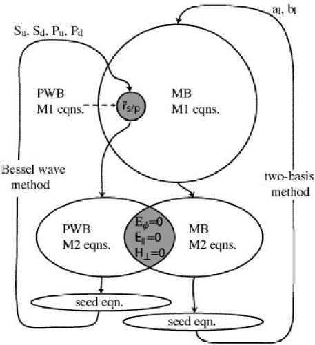
Figure 2: Diagram for the two primary methods. The closed loops suggest the self-consistency or “constructive interference” of the quasimode solutions. Grey regions indicate intersection between PWB and MB methods. Size roughly indicates the “post-basis-derivation work” required to get the equations. The variable coefficients for the vector problem are shown.

4.1 The Scalar Multipole Basis

The scalar MB functions we use are the $\psi_{lm}=j_{l}(kn_{0}r)Y_{lm}(\theta,\phi)$ where $j_{l}$ denotes the spherical Bessel function of the first kind and $Y_{lm}$ is the spherical harmonic function. The scalar MB functions, like the scalar PWB functions, satisfy the wave equation. We assume the field in layer $0$, in a region large enough to encompass the cavity, can be expanded uniquely in terms of the scalar MB functions. Using the cylindrical symmetry of the cavity to solve the problem separately for each value of $m$, we expand the field in the cavity as

$$\psi^{(0)}(\bm{x})=\sum_{l=|m|}^{l_{\text{max}}}c_{l}j_{l}(kn_{0}r)Y_{lm}(\theta,\phi).$$ (48)

The expansion coefficients, $c_{l}$, are complex. One should never need to choose $l_{\text{max}}$ much larger than $\text{Re}(k)n_{0}r_{\text{max}}$ where $r_{\text{max}}$ is the maximum radial extent of the dome (not the hat brim). (Semiclassically, the maximum angular momentum a sphere or hemisphere of radius $R_{s}$ can support (for a given $k$) is $\sim\text{Re}(k)n_{0}R_{s}$, which corresponds to a whispering-gallery mode.)

The scalar MB functions are the exact eigenfunctions of the problem of a hypothetical spherical conductor specified by $r=R_{s}=R$, with eigenvalues given by the zeros of $j_{l}(kn_{0}R)$. The basis functions for which $(l+m)$ is odd are the eigenfunctions of the closed hemispherical conductor. This is because

$$Y_{lm}\text{ has parity }(-1)^{l+m}\text{ in }\cos\theta$$ (49)

and thus is zero at $\theta=\pi/2$. It can also be shown, using the power series expansion of $P_{l}(x)$ given in Ref. ​[13], that $Y_{lm}(\pi/2,\phi)$ is nonzero if $(l+m)$ is even.

4.2 The M1 Equations in the Scalar MB

The expansion of a plane wave in terms of the (monochromatic) scalar MB functions is [10]:

$$e^{\imath\bm{k\cdot x}}=4\pi\sum_{l=0}^{\infty}\sum_{m=-l}^{l}(\imath)^{l}Y_{lm}^{*}(\theta,\phi)j_{l}(kr)Y_{lm}(\theta_{k},\phi_{k}).$$ (50)

The inverse of this relation, the expansion of a scalar MB function in terms of monochromatic plane waves, is

$$j_{l}(kr)Y_{lm}(\theta,\phi)=\int{\textbf{d}}\bm{\Omega}_{k}\left(\frac{(-\imath)^{l}}{4\pi}Y_{lm}(\theta_{k},\phi_{k})\right)e^{\imath\bm{k\cdot x}}.$$ (51)

This equation is easy to verify by inserting (50) into the right hand side. The use of $Y_{lm}=(-1)^{m}Y_{l,-m}^{*}$ and the orthogonality relation for the $Y_{lm}$ leads directly to the left hand side. The expansion (51), applied to layer 0 ($k\rightarrow k_{0}=kn_{0}$), is the foundation for this section and its counterpart for vector fields.

Using (48) and (51) yields the scalar field expansion for a given $m$:

$$\psi^{(0)}= \;\int\text{d}\bm{\Omega}_{k}^{(0)}\,e^{\imath\bm{k}^{(0)}\bm{\cdot x}}\biggl{(}\sum_{l=|m|}c_{l}\frac{(-\imath)^{l}}{4\pi}Y_{lm}(\theta_{k}^{(0)},\phi_{k})\biggr{)}.$$ (52)

The quantity in the curved brackets is $\psi_{k}$, the simple plane wave coefficient (compare to Eqn. (4) with $q$ set to 0). We can now use (35). For $k_{z}>0$, $\psi_{u}=\psi_{k}$ and $\psi_{d}=\psi_{k^{{}^{\prime}}}$, where in cylindrical coordinates $\bm{k^{{}^{\prime}}}=\bm{k^{{}^{\prime}}}(\bm{k})\equiv(k_{\rho},k_{\phi},-k_{z})$. For $k_{z}<0$, $\psi_{d}=\psi_{k}$ and $\psi_{u}=\psi_{k^{{}^{\prime}}}$. Using (49), one gets $\psi_{k^{{}^{\prime}}}=\sum_{l}c_{l}Y_{lm}(\theta_{k}^{(0)},\phi_{k})(-1)^{l+m}(-\imath)^{l}/(4\pi)$. We can now derive an equation that expresses (35) and holds for all $\bm{\Omega}_{k}^{(0)}$:

$$\sum_{l=|m|}c_{l}\frac{(-\imath)^{l}}{4\pi}Y_{lm}(\theta_{k}^{(0)},\phi_{k})\\ \times\left\{\begin{matrix}1-\bar{r}_{s},&l+m\text{ is even}\\ {\textrm{sgn}}(\cos\theta_{k}^{(0)})\left(1+\bar{r}_{s}\right),&l+m\text{ is odd}\end{matrix}\right\}=0.$$ (53)

At this point there are two ways to proceed.

4.2.1 Variant 1

One way to construct the M1 portion of the matrix $A$ is to pick some number $N_{\text{M1 \! dirs}}$ of discrete directions, $\theta_{k}^{(0)}$, and use (53) for each direction (the $\phi_{k}$ dependence divides out). Inspection of the equation reveals that it is even in $\cos\theta_{k}^{(0)}$; thus only polar angles in the domain $[0,\pi/2]$ are needed. Using $\alpha_{k}^{(0)}$ as before to denote this reduced domain, the M1 equations in this variant become:

$$\sum_{l=|m|}^{l_{\text{max}}}c_{l}\frac{(-\imath)^{l}}{4\pi}Y_{lm}(\alpha_{k}^{(0)},0)\\ \times\left(1-(-1)^{l+m}\,r_{s}(\cos\alpha_{k}^{(0)})e^{-\imath 2z_{1}kn_{0}\cos\alpha_{k}^{(0)}}\right)=0.$$ (54)

We note for later comparison that for each $\alpha_{k}^{(0)}$ we need only evaluate a single associated Legendre function (inside the $Y_{lm}$), because the recursive calculation technique for computing $P_{l_{\text{max}}}^{m}(x)$ also computes $P_{l}^{m}(x)$ for $|m|\leq l\leq l_{\text{max}}$. Since each step of this recursive calculation involves a constant number of floating point operations, we may say that the complexity associated with the $P_{l}^{m}$ calculations for each $\alpha_{k}^{(0)}$ is $O(l_{\text{max}}^{2})$. Generally $N_{\text{M1 \! dirs}}\sim l_{\text{max}}$ so the $P_{l}^{m}$ complexity is $O(l_{\text{max}}^{3})$ and the overall number of evaluations of $\bar{r}_{s}$ is $O(l_{\text{max}})$.

4.2.2 Variant 2

Rather than picking discrete directions to turn (53) into many equations, we could project the entire left hand side onto the spherical harmonic basis, $\{Y_{l^{{}^{\prime}}m^{{}^{\prime}}}\}$, (that is, integrate (53) against $Y_{l^{{}^{\prime}}m^{{}^{\prime}}}^{*}(\bm{\Omega}_{k}^{(0)})$ in $\bm{\Omega}_{k}^{(0)}$). Due to the uniqueness of the basis expansion, the integral for each $(l^{{}^{\prime}},m^{{}^{\prime}})$ pair must be zero. The integrals for $m^{{}^{\prime}}\neq m$ are zero and can be neglected. Thus the number of equations generated is $N_{l^{{}^{\prime}}}=l_{\text{max}}^{{}^{\prime}}-|m|+1$. We set $l_{\text{max}}^{{}^{\prime}}=l_{\text{max}}$.

Since (53) is even in $\cos\theta_{k}^{(0)}$, integrating against $Y_{l^{{}^{\prime}}m}^{*}$ gives $0$ if $l^{{}^{\prime}}+m$ is odd, halving the number of equations. When $l^{{}^{\prime}}+m$ is even the integration must be done numerically. The most analytically simplified version of the coefficients of $c_{l}$ in the M1 equation corresponding to $l^{{}^{\prime}}$ (for $l^{{}^{\prime}}+m$ even) is:

$$\text{M1}_{l^{{}^{\prime}},l}=\zeta\int_{0}^{1}P_{l}^{|m|}(x)P_{l^{{}^{\prime}}}^{|m|}(x)\left(1-(-1)^{l+m}\bar{r}_{s}(x)\right)\text{d}x,$$ (55)

where

$$\zeta\equiv\frac{(-\imath)^{l}}{4\pi}\!\left((2l+1)(2l^{{}^{\prime}}+1)\frac{(l-|m|)!}{(l+|m|)!}\frac{(l^{{}^{\prime}}-|m|)!}{(l^{{}^{\prime}}+|m|)!}\right)^{1/2}.$$ (56)

This comes from using the properties of $Y_{lm}$ under a sign change of $m$, using the definition of $Y_{lm}$, doing the $\phi_{k}$ integral, and halving the domain of the even integral over $x=\cos\alpha_{k}^{(0)}$. Noting that the number of unknowns in the solution vector $\bm{y}$ is $N_{l}=l_{\text{max}}-|m|+1$, the number of (complex) coefficients that must be calculated is about $N_{l}^{2}/2$. Noting that $\text{M1}_{l,l^{{}^{\prime}}}=(-\imath)^{l^{{}^{\prime}}-l}\text{M1}_{l^{{}^{\prime}},l}$ when $l+m$ and $l^{{}^{\prime}}+m$ are both even, the calculation is reduced to about $3N_{l}^{2}/4$ real-valued integrations.

While this variant of the method is in some ways the most elegant, the numerical integrals are extremely computationally intensive. Our implementation used an adaptive Gaussian quadrature function, gsl_integration_qag of the GSL. (Adaptive algorithms choose a different set of evaluation points for each integration and achieve a prescribed accuracy; in a sense the integral is done in a continuous rather than a discrete manner.) For an adaptive algorithm, the complexity associated with the $P_{l}^{m}$ calculation is $O(l_{\text{max}}^{3+\nu})$, where $\nu\geq 1$. The number of evaluations of $\bar{r}_{s}$ is $O(l_{\text{max}}^{2+\nu})$. In practice, variant 2 is much slower than variant 1 even for cavities as small as $R/\lambda\approx 5$ with simple mirrors. Checking between the two variants has generally shown very good agreement.

4.3 The Linear System of Equations in the Scalar MB

The M1 equations have been given in the previous section. Using (48) yields an M2 equation

$$\sum_{l=|m|}^{l_{\text{max}}}c_{l}j_{l}(kn_{0}r_{*})Y_{lm}(\theta_{*},0)=0,$$ (57)

for each location $(r_{*},\theta_{*})$. The discussions from Section 3.3 regarding the M2 equations, the seed equation, and the method of solution to $A\bm{y}=\bm{b}$ apply here. The number of columns in $A$ is $N_{l}$ and the number of rows is $(N_{\text{M1 dirs}}+N_{\text{M2 loc}}+1)$ for variant 1 or about $(N_{l}/2+N_{\text{M2 loc}}+1)$ for variant 2.

4.4 Calculating the Field in the Layers with the Scalar MB

To calculate the complex field anywhere in layer $0$ once a quasimode solution $\bm{y}$ has been found, Eqn. (48) can be used directly. To calculate the field in the layers below the cavity ($q>0$) where the expansion does not apply, the Bessel waves must be used, along with the $T_{s}^{(q)}$ matrix that propagates them. Performing the $\phi_{k}$ integration in (52), using (49), and then comparing with (9) and (25) with $q=0$ in both of these yields the Bessel wave coefficients:

$$\psi_{u}^{(0)} =\sum_{l}c_{l}\frac{(-\imath)^{l}}{4\pi}Y_{lm}(\alpha_{k}^{(0)},0),$$

$$\psi_{d}^{(0)} =\sum_{l}c_{l}\frac{(-\imath)^{l}}{4\pi}Y_{lm}(\alpha_{k}^{(0)},0)(-1)^{l+m}.$$ (58)

Now (25) can be used with $q>0$ yielding

$$\psi^{(q)}(\bm{x})= \;\frac{(\imath)^{m}}{2}e^{\imath m\phi}\int_{0}^{\pi/2}\text{d}\alpha_{k}^{(0)}\sin(\alpha_{k}^{(0)})$$

$$\times J_{m}(\rho kn_{0}\sin\alpha_{k}^{(0)})\Bigl{[}\sum_{l}c_{l}(-\imath)^{l}Y_{lm}(\alpha_{k}^{(0)},0)$$

$$\times\left(\,{}_{+}\beta_{s}^{(q)}+(-1)^{l+m}\,_{+}\gamma_{s}^{(q)}\right)\Bigr{]}.$$ (59)

This is a costly numerical integration to do with an adaptive algorithm. For every sampled $\alpha_{k}^{(0)}$, the quantities $T_{s}$, $P_{l_{\text{max}}}^{m}$ and $J_{m}$ must be calculated once. For displaying large regions of the field in the stack, it is sufficiently accurate to simply convert the solved MB solution vector $\bm{y}$ into a PWB solution vector (with $N_{\text{dirs}}\sim l_{\text{max}}$) by means of a separate program using (58), and then use the discrete form of (25) to plot.

4.5 The Vector Multipole Basis

We expand the electromagnetic field in layer $0$ (at least in a finite region surrounding the cavity) in the vector multipole basis using spherical Bessel functions of the first kind ($j_{l}$). The multipole basis uses the vector spherical harmonics (VSH; same abbreviation for singular), which are given by[14]

$$\bm{M}_{lm}(\bm{x}) =-j_{l}(kn_{0}r)\,\bm{x\times\nabla}Y_{lm}(\theta,\phi),$$

$$\bm{N}_{lm}(\bm{x}) =\frac{1}{kn_{0}}\bm{\nabla\times M}_{lm}.$$ (60)

The VSH are not defined for $l=0$. The nature of the electromagnetic multipole expansion is developed in section 9.7 of the book by Jackson[10] using somewhat different terminology. The multipole expansion of the electromagnetic fields is

$$\bm{E}^{(0)}(\bm{x}) =\sum_{l=l_{\text{min}}}^{l_{\text{max}}}\left(-a_{l}\bm{N}_{lm}+\imath b_{l}\bm{M}_{lm}\right),$$

$$\bm{H}^{(0)}(\bm{x}) =\tilde{n}_{0}\sum_{l=l_{\text{min}}}^{l_{\text{max}}}\left(\imath a_{l}\bm{M}_{lm}+b_{l}\bm{N}_{lm}\right),$$ (61)

where cylindrical symmetry has been invoked to remove the sum over $m$, and $l_{\text{min}}=\max(1,|m|)$. The $a_{l}$ and $b_{l}$ are complex coefficients and there are $N_{l}=l_{\text{max}}-l_{\text{min}}+1$ of each of them. The $a_{l}$ coefficients correspond to electric multipoles and the $b_{l}$ coefficients correspond to magnetic multipoles. The explicit forms of the VSH are

$$\bm{M}_{lm}(\bm{x})= \;\hat{\bm{\theta}}\left(\frac{\imath m}{\sin\theta}j_{l}(kn_{0}r)Y_{lm}(\theta,\phi)\right)$$

$$+\hat{\bm{\phi}}\left(-j_{l}(kn_{0}r)\frac{\partial}{\partial\theta}Y_{lm}(\theta,\phi)\right),$$

$$\bm{N}_{lm}(\bm{x})= \;\hat{\bm{r}}\left(\frac{l(l+1)}{kn_{0}r}j_{l}(kn_{0}r)Y_{lm}(\theta,\phi)\right)$$

$$+\hat{\bm{\theta}}\left(\frac{1}{kn_{0}r}\frac{\partial}{\partial r}\left(rj_{l}(kn_{0}r)\right)\frac{\partial}{\partial\theta}Y_{lm}(\theta,\phi)\right)$$

$$+\hat{\bm{\phi}}\left(\frac{\imath m}{kn_{0}r\sin\theta}\frac{\partial}{\partial r}\left(rj_{l}(kn_{0}r)\right)Y_{lm}(\theta,\phi)\right).$$ (62)

4.6 The M1 Equations in the Vector MB

The goal of the calculation here is to transform the M1 relations, (38) and (40), into equations such that each dot product is written in the form $\sum_{l}(a_{l}f_{a}(\bm{k})+b_{l}f_{b}(\bm{k}))$. The resulting (two) equations will be the vector analogues of (53) and will hold for all $\bm{\Omega}_{k}^{(0)}$, leading to two variants of solution method in the same manner as before. First we must Fourier expand $\bm{E}^{(0)}$ as we expanded $\psi^{(0)}$ to get (52). The only Fourier relation we have is (51) which expands the quantity $j_{l}Y_{lm}(\bm{x})$. We must therefore break $\bm{M}_{lm}$ into terms containing this quantity.

Here we can make use of the orbital angular momentum operator $\bm{L}=-\imath(\bm{x\times\nabla})$. Using the ladder operators, $L_{\pm}=L_{x}\pm\imath L_{y}$, the VSH $\bm{M}_{lm}=-\imath j_{l}\bm{L}Y_{lm}$ can be shown to be

$$\bm{M}_{lm}= \;\left(-\imath j_{l}\right)\times\Bigl{[}\hat{\bm{x}}\frac{1}{2}\left(d_{lm}^{+}Y_{lm+1}+d_{lm}^{-}Y_{lm-1}\right)$$

$$+\hat{\bm{y}}\frac{\imath}{2}\left(-d_{lm}^{+}Y_{lm+1}+d_{lm}^{-}Y_{lm-1}\right)+\hat{\bm{z}}\left(mY_{lm}\right)\Bigr{]},$$ (63)

where

$$d_{lm}^{\pm}\equiv\sqrt{(l\mp m)(l\pm m+1)}.$$ (64)

Using (51) multiple times yields

$$\bm{M}_{lm}=\int{\textbf{d}}\bm{\Omega}_{k}^{(0)}\tilde{\bm{M}}_{lm}e^{\imath\bm{k}^{(0)}\bm{\cdot x}},$$ (65)

with

$$\tilde{\bm{M}}_{lm}= \;\hat{\bm{x}}\frac{(-\imath)^{l}}{8\pi}(-\imath)e_{lm}^{+}+\hat{\bm{y}}\frac{(-\imath)^{l}}{8\pi}(-1)e_{lm}^{-}$$

$$+\hat{\bm{z}}\frac{(-\imath)^{l}}{4\pi}mY_{lm}(\bm{\Omega}_{k}^{(0)}),$$ (66)

where

$$e_{lm}^{\pm}\equiv d_{lm}^{+}Y_{lm+1}(\bm{\Omega}_{k}^{(0)})\pm d_{lm}^{-}Y_{lm-1}(\bm{\Omega}_{k}^{(0)}).$$ (67)

We can avoid the task of expanding $\bm{N}_{lm}$ into $j_{l}Y_{lm}$ terms by just using

$$\bm{N}_{lm}=\frac{\bm{\nabla\times M}_{lm}}{kn_{0}}=\int\!{\textbf{d}}\bm{\Omega}_{k}^{(0)}\frac{\imath}{kn_{0}}\bm{k}^{(0)}\bm{\times}\tilde{\bm{M}}_{lm}e^{\imath\bm{k}^{(0)}\bm{\cdot x}}.$$ (68)

Performing the cross product and substituting into (61) using (65-66) yields

$$E_{x}(\bm{x})= \;\int{\textbf{d}}\bm{\Omega}_{k}^{(0)}\,e^{\imath\bm{k}^{(0)}\bm{\cdot x}}\biggl{\{}\sum_{l}\frac{(-\imath)^{l}}{4\pi}\biggl{[}a_{l}\Bigl{(}-m\sin\theta_{k}^{(0)}\sin\phi_{k}Y_{lm}-\frac{\imath}{2}\cos\theta_{k}^{(0)}\,e_{lm}^{-}\Bigr{)}+b_{l}\Bigl{(}\frac{1}{2}e_{lm}^{+}\Bigr{)}\biggr{]}\biggr{\}},$$

$$E_{y}(\bm{x})= \;\int{\textbf{d}}\bm{\Omega}_{k}^{(0)}\,e^{\imath\bm{k}^{(0)}\bm{\cdot x}}\biggl{\{}\sum_{l}\frac{(-\imath)^{l}}{4\pi}\biggl{[}a_{l}\Bigl{(}m\sin\theta_{k}^{(0)}\cos\phi_{k}Y_{lm}-\frac{1}{2}\cos\theta_{k}^{(0)}\,e_{lm}^{+}\Bigr{)}+b_{l}\Bigl{(}\frac{-\imath}{2}e_{lm}^{-}\Bigr{)}\biggr{]}\biggr{\}},$$

$$E_{z}(\bm{x})= \;\int{\textbf{d}}\bm{\Omega}_{k}^{(0)}\,e^{\imath\bm{k}^{(0)}\bm{\cdot x}}\biggl{\{}\sum_{l}\frac{(-\imath)^{l}}{4\pi}\biggl{[}a_{l}\Bigl{(}\frac{\imath}{2}\sin\theta_{k}^{(0)}\cos\phi_{k}\,e_{lm}^{-}+\frac{1}{2}\sin\theta_{k}^{(0)}\sin\phi_{k}\,e_{lm}^{+}\Bigr{)}+b_{l}\Bigl{(}mY_{lm}\Bigr{)}\biggr{]}\biggr{\}},$$ (69)

where $Y_{lm}$ is understood to mean $Y_{lm}(\bm{\Omega}_{k}^{(0)})$. The quantities inside the curly braces in (69) will be denoted by $\tilde{E}_{x}(\bm{k})$, $\tilde{E}_{y}(\bm{k})$, and $\tilde{E}_{z}(\bm{k})$, where the “(0)” superscript on $\bm{k}$ has been dropped. We will also need $\tilde{\bm{E}}(\bm{k^{{}^{\prime}}})$ where $\bm{k^{{}^{\prime}}}(\bm{k})=(k_{\rho},k_{\phi},-k_{z})$ as before. Again using (49) we find

$$\tilde{E}_{x}(\bm{k^{{}^{\prime}}})= \;\sum_{l}\frac{(-\imath)^{l}}{4\pi}(-1)^{l+m}\biggl{[}a_{l}\Bigl{(}-m\sin\theta_{k}^{(0)}\sin\phi_{k}Y_{lm}-\frac{\imath}{2}\cos\theta_{k}^{(0)}\,e_{lm}^{-}\Bigr{)}+b_{l}\Bigl{(}\frac{-1}{2}e_{lm}^{+}\Bigr{)}\biggr{]},$$

$$\tilde{E}_{y}(\bm{k^{{}^{\prime}}})= \;\sum_{l}\frac{(-\imath)^{l}}{4\pi}(-1)^{l+m}\biggl{[}a_{l}\Bigl{(}m\sin\theta_{k}^{(0)}\cos\phi_{k}Y_{lm}-\frac{1}{2}\cos\theta_{k}^{(0)}\,e_{lm}^{+}\Bigr{)}+b_{l}\Bigl{(}\frac{\imath}{2}e_{lm}^{-}\Bigr{)}\biggr{]},$$

$$\tilde{E}_{z}(\bm{k^{{}^{\prime}}})= \;\sum_{l}\frac{(-\imath)^{l}}{4\pi}(-1)^{l+m}\biggl{[}a_{l}\Bigl{(}\frac{-\imath}{2}\sin\theta_{k}^{(0)}\cos\phi_{k}\,e_{lm}^{-}+\frac{-1}{2}\sin\theta_{k}^{(0)}\sin\phi_{k}\,e_{lm}^{+}\Bigr{)}+b_{l}\Bigl{(}mY_{lm}\Bigr{)}\biggr{]}.$$ (70)

4.6.1 The M1 equations for s-polarization

We will now define $f_{lm}$ and $g_{lm}$ by

$$\tilde{\bm{E}}(\bm{k})\bm{\cdot\epsilon}_{s,k}\equiv\sum_{l}\frac{(-\imath)^{l}}{4\pi}\left(a_{l}g_{lm}+b_{l}f_{lm}\right).$$ (71)

Performing the dot product using (11) yields

$$f_{lm}= \;\frac{\imath}{2}\left(d_{lm}^{+}Y_{lm+1}e^{-\imath\phi_{k}}-d_{lm}^{-}Y_{lm-1}e^{\imath\phi_{k}}\right),$$

$$g_{lm}= \;\frac{1}{2}\cos\theta_{k}^{(0)}\left(d_{lm}^{+}Y_{lm+1}e^{-\imath\phi_{k}}+d_{lm}^{-}Y_{lm-1}e^{\imath\phi_{k}}\right)$$

$$-m\sin\theta_{k}^{(0)}Y_{lm}$$

$$= \;\frac{1}{2}\sqrt{\frac{2l+1}{2l-1}}\biggl{(}\sqrt{(l-m)(l-m-1)}Y_{l-1,m+1}e^{-\imath\phi_{k}}$$

$$+\sqrt{(l+m)(l+m-1)}Y_{l-1,m-1}e^{\imath\phi_{k}}\biggr{)}.$$ (72)

The simplification in the last step has been done using recursion relations for the $P_{l}^{m}$. Performing the dot product for $\tilde{\bm{E}}(\bm{k^{{}^{\prime}}})$ yields

$$\tilde{\bm{E}}(\bm{k^{{}^{\prime}}})\bm{\cdot\epsilon}_{s,k}=\sum_{l}\frac{(-\imath)^{l}}{4\pi}(-1)^{l+m}\left(a_{l}g_{lm}-b_{l}f_{lm}\right).$$ (73)

The M1 relation (from (38)) is $\tilde{\bm{E}}(\bm{k})\bm{\cdot\epsilon}_{s,k}=\bar{r}_{s}\tilde{\bm{E}}(\bm{k^{{}^{\prime}}})\bm{\cdot\epsilon}_{s,k}$ for $k_{z}>0$ and $\tilde{\bm{E}}(\bm{k^{{}^{\prime}}})\bm{\cdot\epsilon}_{s,k}=\bar{r}_{s}\tilde{\bm{E}}(\bm{k})\bm{\cdot\epsilon}_{s,k}$ for $k_{z}<0$. These lead to an M1 equation that holds for all $\bm{\Omega}_{k}^{(0)}$:

$$\sum_{l=l_{\text{min}}}^{l_{\text{max}}}\frac{(-\imath)^{l}}{4\pi}\left\{\begin{matrix}a_{l}s_{1}g_{lm}+b_{l}s_{2}f_{lm},&l+m\text{ even}\\ a_{l}s_{2}g_{lm}+b_{l}s_{1}f_{lm},&l+m\text{ odd}\end{matrix}\right\}=0,$$ (74)

where $s_{1}\equiv 1-\bar{r}_{s}(|\cos\theta_{k}^{(0)}|)$ and $s_{2}\equiv{\textrm{sgn}}(\cos\theta_{k}^{(0)})(1+\bar{r}_{s}(|\cos\theta_{k}^{(0)}|))$.

4.6.2 The M1 equations for p-polarization

The M1 equation for p-polarization is obtained the same way as above. The calculation is simplified by temporarily switching phase conventions. We define the unit vector $\tilde{\bm{\epsilon}}_{p,k}\equiv{\textrm{sgn}}(\cos\theta_{k}^{(0)})\bm{\epsilon}_{p,k}$ (using (11)) so that

$$\tilde{\bm{\epsilon}}_{p,k}= \;\hat{\bm{x}}\cos\theta_{k}^{(0)}\cos\phi_{k}+\hat{\bm{y}}\cos\theta_{k}^{(0)}\sin\phi_{k}-\hat{\bm{z}}\sin\theta_{k}^{(0)},$$

$$\tilde{\bm{\epsilon}}_{p,k^{{}^{\prime}}}= \;-\hat{\bm{x}}\cos\theta_{k}^{(0)}\cos\phi_{k}-\hat{\bm{y}}\cos\theta_{k}^{(0)}\sin\phi_{k}-\hat{\bm{z}}\sin\theta_{k}^{(0)}.$$ (75)

The M1 relation is now $\tilde{\bm{E}}(\bm{k})\bm{\cdot}\tilde{\bm{\epsilon}}_{p,k}=(-\bar{r}_{p})\tilde{\bm{E}}(\bm{k^{{}^{\prime}}})\bm{\cdot}\tilde{\bm{\epsilon}}_{p,k^{{}^{\prime}}}$ for $k_{z}>0$ and $\tilde{\bm{E}}(\bm{k^{{}^{\prime}}})\bm{\cdot}\tilde{\bm{\epsilon}}_{p,k^{{}^{\prime}}}=(-\bar{r}_{p})\tilde{\bm{E}}(\bm{k})\bm{\cdot}\tilde{\bm{\epsilon}}_{p,k}$ for $k_{z}<0$, where $\bar{r}_{p}$ has not changed in any way. Performing the dot products, we find that

$$\tilde{\bm{E}}(\bm{k})\bm{\cdot}\tilde{\bm{\epsilon}}_{p,k}= \;\sum_{l}\frac{(-\imath)^{l}}{4\pi}(-a_{l}f_{lm}+b_{l}g_{lm}),$$

$$\tilde{\bm{E}}(\bm{k^{{}^{\prime}}})\bm{\cdot}\tilde{\bm{\epsilon}}_{p,k^{{}^{\prime}}}= \;\sum_{l}\frac{(-\imath)^{l}}{4\pi}(-1)^{l+m}(a_{l}f_{lm}+b_{l}g_{lm}).$$ (76)

This leads to the M1 equation for p-polarization which holds for all $\bm{\Omega}_{k}^{(0)}$:

$$\sum_{l=l_{\text{min}}}^{l_{\text{max}}}\frac{(-\imath)^{l}}{4\pi}\biggl{\{}\begin{matrix}-a_{l}p_{2}f_{lm}+b_{l}p_{1}g_{lm},&l+m\text{ even}\\ -a_{l}p_{1}f_{lm}+b_{l}p_{2}g_{lm},&l+m\text{ odd}\end{matrix}\biggr{\}}=0,$$ (77)

where $p_{1}\equiv 1+\bar{r}_{p}(|\cos\theta_{k}^{(0)}|)$ and $p_{2}\equiv{\textrm{sgn}}(\cos\theta_{k}^{(0)})(1-\bar{r}_{p}(|\cos\theta_{k}^{(0)}|))$.

4.6.3 Variant 1

Variant 1 for the vector case proceeds exactly as it does for the scalar case. The M1 equations (74) and (77) are seen to be even in $\cos\theta_{k}^{(0)}$, allowing us to pick directions only in the domain $[0,\pi/2]$. Thus for each discrete direction $\alpha_{k}^{(0)}$ we get one equation (in the M1 portion of $A$) for each polarization. No modification of (74) or (77) is needed, except that we can take $\phi_{k}=0$ and $\cos\theta_{k}^{(0)}=\cos\alpha_{k}^{(0)}\geq 0$.

The complexity of calculating the M1 portion of $A$ is of the same order in $l_{\text{max}}$ as it is for the scalar MB. However, numerous constant factors make the computation time an order of magnitude longer, as there are more $P_{l}^{m}$ functions to compute and $\bar{r}_{p}$ must be computed in addition to $\bar{r}_{s}$.

4.6.4 Variant 2

In this minor section, we assume that $m\geq 0$ (see Appendix B for plotting negative $m$ modes from positive $m$ solutions). We follow the same procedure used in variant 2 for the scalar field. Integrating (74) and (77) against $Y_{l^{{}^{\prime}}m^{{}^{\prime}}}(\bm{\Omega}_{k}^{(0)})$ yields zero if either $m^{{}^{\prime}}\neq m$ or $l^{{}^{\prime}}+m$ is odd. For $m^{{}^{\prime}}=m$ and $l^{{}^{\prime}}+m$ even, the M1 equation associated with each $l^{{}^{\prime}}$ in $\{|m|,|m|+1,\ldots,l_{\text{max}}\}$ for s-polarization is

$$\sum_{l=l_{\text{min}}}^{l_{\text{max}}}-\frac{1}{2}\zeta\,\biggl{[}a_{l}\int_{0}^{1}\Bigl{(}1-(-1)^{l+m}\,\bar{r}_{s}\Bigr{)}\Bigl{(}P_{l-1}^{m+1}(x)+(l+m)(l+m-1)P_{l-1}^{m-1}(x)\Bigr{)}P_{l^{{}^{\prime}}}^{m}(x)\,\text{d}x\\ +b_{l}(\imath)\int_{0}^{1}\Bigl{(}1+(-1)^{l+m}\,\bar{r}_{s}\Bigr{)}\Bigl{(}P_{l}^{m+1}(x)-(l+m)(l-m+1)P_{l}^{m-1}(x)\Bigr{)}P_{l^{{}^{\prime}}}^{m}(x)\,\text{d}x\biggr{]}=0,$$ (78)

and the M1 equation for p-polarization is

$$\sum_{l=l_{\text{min}}}^{l_{\text{max}}}-\frac{1}{2}\zeta\,\biggl{[}a_{l}(-\imath)\int_{0}^{1}\Bigl{(}1-(-1)^{l+m}\,\bar{r}_{p}\Bigr{)}\Bigl{(}P_{l}^{m+1}(x)-(l+m)(l-m+1)P_{l}^{m-1}(x)\Bigr{)}P_{l^{{}^{\prime}}}^{m}(x)\,\text{d}x\\ +b_{l}\int_{0}^{1}\Bigl{(}1+(-1)^{l+m}\,\bar{r}_{p}\Bigr{)}\Bigl{(}P_{l-1}^{m+1}(x)+(l+m)(l+m-1)P_{l-1}^{m-1}(x)\Bigr{)}P_{l^{{}^{\prime}}}^{m}(x)\,\text{d}x\biggr{]}=0,$$ (79)

where $P_{\mu}^{n}=0$ for $|n|>\mu$. Note that if $m=0$ the equations for $l^{{}^{\prime}}=0$ are included. We implemented this by calculating an array of each of the following types of integrals:

$$\begin{matrix}\int_{0}^{1}P_{\mu}^{m+1}P_{\nu}^{m}\,\text{d}x,&\int_{0}^{1}P_{\mu}^{m-1}P_{\nu}^{m}\,\text{d}x,\\ \int_{0}^{1}P_{\mu}^{m+1}P_{\nu}^{m}\bar{r}_{s}\,\text{d}x,&\int_{0}^{1}P_{\mu}^{m-1}P_{\nu}^{m}\bar{r}_{s}\,\text{d}x,\\ \int_{0}^{1}P_{\mu}^{m+1}P_{\nu}^{m}\bar{r}_{p}\,\text{d}x,&\int_{0}^{1}P_{\mu}^{m-1}P_{\nu}^{m}\bar{r}_{p}\,\text{d}x.\end{matrix}$$

The integrals in the first row can be calculated ahead of time and stored in a data file. The other integrals must be calculated each time the matrix $A$ is calculated. The complexity of the calculation is of the same order in $l_{\text{max}}$ as for variant 2 in the scalar case. These integrals are very numerically intensive and in practice variant 2 takes much longer than variant 1. We have found good agreement between the two variants, indicating that variant 1 can be used all or most of the time.

4.7 The Linear System of Equations in the Vector MB

The M2 equations are found in the usual way, choosing locations $(\rho_{*},\theta_{*})$ with $\phi=0$ and constructing the equations $E_{\phi}=0$, $E_{\parallel}=E_{\rho}\cos\eta-E_{z}\sin\eta=0$, and $H_{\perp}=H_{\rho}\sin\eta+H_{z}\cos\eta=0$. The fields $\bm{E}$ and $\bm{H}$ are found by substituting (62) into (61). The derivatives in (62) are

$$\frac{\partial}{\partial r}(rj_{l}(kn_{0}r))=kn_{0}rj_{l-1}(kn_{0}r)-lj_{l}(kn_{0}r),$$ (80)

and, for $m\geq 0$,

$$\frac{\partial}{\partial\theta}Y_{lm}(\theta,\phi)=\frac{1}{2}\left[\frac{(2l+1)(l-m)!}{4\pi(l+m)!}\right]^{1/2}\\ \times\left(P_{l}^{m+1}-(l+m)(l-m+1)P_{l}^{m-1}\right)e^{\imath m\phi},$$ (81)

where $P_{l}^{l+1}=0$. (For negative $m$ use $Y_{l,-m}=(-1)^{m}Y_{lm}^{*}$.) The number of columns in $A$ is $2N_{l}$ and the number of rows is $(2N_{\text{M1 dirs}}+3N_{\text{M2 loc}}+1)$ for variant 1 and about $(N_{l}+3N_{\text{M2 loc}}+1)$ for variant 2.

4.8 Calculating the Field in the Layers with the Vector MB

To calculate the field in layer $0$, the expansion (61) is used directly, with (62), (80), and (81) being used to obtain the explicit form. As for the scalar case, there is no direct expansion for the layers $q>0$ in the MB, and we must use the Bessel wave basis. Using (71), (73), and (76), the conversion is seen to be

$$S_{u} =\sum_{l=l_{\text{min}}}^{l_{\text{max}}}\frac{(-\imath)^{l}}{4\pi}\left(a_{l}g_{lm}+b_{l}f_{lm}\right)\biggl{|}_{\theta_{k}^{(0)}=\alpha_{k}^{(0)},\phi_{k}=0},$$

$$S_{d} =\sum_{l}\frac{(-\imath)^{l}}{4\pi}(-1)^{l+m}\left(a_{l}g_{lm}-b_{l}f_{lm}\right)\biggl{|}_{\theta_{k}^{(0)}=\alpha_{k}^{(0)},\phi_{k}=0},$$

$$P_{u} =\sum_{l}\frac{(-\imath)^{l}}{4\pi}\left(-a_{l}f_{lm}+b_{l}g_{lm}\right)\biggl{|}_{\theta_{k}^{(0)}=\alpha_{k}^{(0)},\phi_{k}=0},$$

$$P_{d} =\sum_{l}\frac{(-\imath)^{l}}{4\pi}(-1)^{l+m}\left(a_{l}f_{lm}+b_{l}g_{lm}\right)\biggl{|}_{\theta_{k}^{(0)}=\alpha_{k}^{(0)},\phi_{k}=0}.$$ (82)

This is the vector case analogue of Eqn. (58).

At this point the Bessel wave coefficients $S_{u}$, etc., are continuous functions of $\alpha_{k}^{(0)}$, not discrete as they were in the Bessel wave method. These continuous coefficients are substituted into the integrals (32), and finally (30) is used to give the vector fields in the layers. As in the scalar case, however, doing the integrals with an adaptive algorithm is impractical if one is plotting the vector fields in a sizable region. In this case, it is best to make the Bessel wave coefficients discrete and use a simple integration method, or, as was suggested in the scalar case, to pick a $N_{\text{dirs}}$ and create a PWB solution vector that can then be plotted via a PWB plotting routine.

5 Demonstrations and Comparisons

In this section we will demonstrate, but not thoroughly analyze, several results that we have obtained using our model and methods. The modes shown here all have $\Delta_{n}<0.0002$ and do not contain large amounts of high-angle plane waves, which in principle can cause problems (see Appendix A.1). The authors expect to publish a separate paper focusing on the modes themselves. In this section we will also compare our implementations of the two-basis method and the Bessel wave method. Before reading this section it may be helpful to look at Appendix B.

5.1 The “V” Mode: A Stack Effect

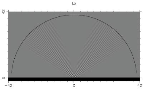
Figure 3: Contrast-enhanced plot of $\text{Re}E_{x}$ in the $y$-$z$ plane for a “V” mode ($m=1,k=8.1583-\imath 0.000019$). M2 is spherical and origin-centered; $R=40$; $z_{1}=0.3$; $z_{e}=3$; M1 = stack II; $k_{s}=8.1600$; $N_{s}=20$. In this and other side view plots, the field outside the cavity has been set to zero.

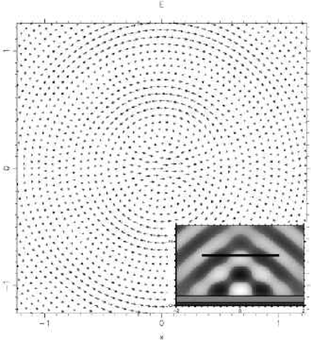
Figure 4: An $x$-$y$ cross section of the mode in Fig. ​3 at $z=1.58$. Units are in $\mu$m as usual. For $m=+1$, the forward time evolution is simply the counter-clockwise rotation of the entire vector field. If $m=+1$ and $m=-1$ are mixed to create a cosine mode, the arrow directions remain fixed and their lengths simply oscillate sinusoidally in time so that the mode is associated with $x$ polarization. The inset shows the location of the cross section in the view of Fig. ​3. (The field is plotted only in layer 0.)

As mentioned several times in the Introduction, the correct treatment of a dielectric stack can be essential for getting results that are even qualitatively correct. One of the most remarkable differences that we have observed when switching from simple to dielectric M1 mirrors occurs right where someone looking for highly-focused, drivable modes would be interested: the widening behavior of the fundamental Gaussian mode (the 00 mode). A Gaussian mode of a near-hemispherical cavity will become more and more focused (wide at the curved mirror and narrow at the flat mirror) as $z_{1}$ is decreased (from a starting value for which the Gaussian mode is paraxial). As the mode becomes more focused, of course, the paraxial approximation becomes less valid and at some point Gaussian theory no longer applies. We have found, using realistic Al_1-xGa_xAs–AlAs stack models (stacks I and II described in Appendix C), that the 00 mode splits into two parts, so that in the side view a “V” shape is formed. Figure 3 shows a split mode and Fig. ​4 shows the physical transverse electric field, $\text{Re}\bm{E}_{T}\equiv\text{Re}E_{x}\hat{\bm{x}}+\text{Re}E_{y}\hat{\bm{y}}$, for this mode near the focal region. Figure 5 shows the values of $\text{Re}(kR)$ as $z_{1}$ is changed from 0.3 to about 0.63. Figure 6 shows a zoomed view of the field at the focus of the mode at $z_{1}=0.63$, where it is qualitatively a 00 mode. If a conducting mirror is used, the central cone simply grows wider and wider, but does not split. The V mode is predominately s-polarized and appears in the scalar problem as well. Thus it appears that the V mode is a result of the non-constancy of $\arg(r_{s}(\alpha))$ for a dielectric stack. We note here that following the 00 mode as $z_{1}$ is changed is an imperfect process: it is possible that the following procedure may skip over narrow anticrossings that are difficult to resolve. However, the character of the mode is maintained through such anticrossings.

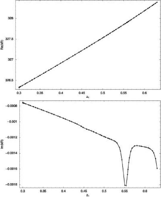
Figure 5: Following $kR$ as $z_{1}$ is varied. The points of the two graphs correspond one-to-one, with the parameter $z_{1}$ increasing from left to right in both graphs. The peaks in resonance width have not yet been analyzed.

The apparent splitting of the central cone/lobe for higher order Gaussian modes has also been observed. In the next section we look at some higher order Gaussian modes, focusing not on what occurs at the breaking of the paraxial condition, but on what is allowed and observed for modes that are very paraxial.

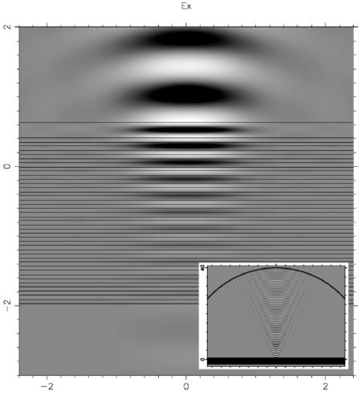
Figure 6: The field in layers 0–X for the mode at $z_{1}=0.63$. The inset shows the entire mode. The “V” nature of the mode has been lost as it has become more paraxial and more like the fundamental Gaussian. $\text{Re}\bm{E}_{T}$ everywhere lies nearly in a single direction at any instant (here it is in the $x$ direction). The $x$-$z$ plane is shown here, although the plots of $E_{x}$ in any plane containing the $z$ axis are very similar. Here $k=8.2098-\imath 0.0000401$.

5.2 Persistent Stack-Induced Mixing of Near-Degenerate Laguerre-Gaussian Mode Pairs

As mentioned in the previous section, we do observe the fundamental Gaussian mode for paraxial cavities with both dielectric and conducting planar mirrors. The situation becomes more interesting when we look at higher order Gaussian modes. It is true that, as modes become increasingly paraxial, Gaussian theory must apply. However, the way in which it applies allows the design of M1 to play a significant role. Here we will demonstrate the ability of a dielectric stack (stack II) to mix near-degenerate pairs predicted by Gaussian theory into new, more complicated near-degenerate pairs of modes. We must provide considerable background to put these modes into context. Our discussion applies to modes with paraxial geometry, modes for which the paraxial parameter $h\equiv\lambda/(\pi w_{0})=w_{0}/z_{R}$ is much less than 1. (Here $w_{0}$ is the waist radius and $z_{R}$ is the Rayleigh range, as used in standard Gaussian theory.) In this section, the solutions we are referring to are always the $+m$ or $-m$ modes discussed in Appendix B, and never mixtures of these, such as the cosine and sine modes discussed in the same section.

5.2.1 Paraxial Theory for Vector Fields

From Gaussian theory, using the Laguerre-Gaussian (LG) basis, we expect that the transverse electric field of any mode in the paraxial limit is expressible in the form:

$$\bm{E}_{T}=\sum_{j=0}^{N}\Bigl{[}A_{j}^{+}\Bigl{(}\begin{smallmatrix}1\\ \imath\end{smallmatrix}\Bigr{)}+A_{j}^{-}\Bigl{(}\begin{smallmatrix}1\\ -\imath\end{smallmatrix}\Bigr{)}\Bigr{]}\text{LG}_{\min(j,N-j)}^{2j-N}(\bm{x}).$$ (83)

Here $N\geq 0$ is the order of the mode. The $A_{j}^{\pm}$ are complex coefficients and $\bigl{(}\begin{smallmatrix}1\\ \imath\end{smallmatrix}\bigr{)}$ and $\bigl{(}\begin{smallmatrix}1\\ -\imath\end{smallmatrix}\bigr{)}$ are the Jones’ vectors for right and left circular polarization, respectively. The explicit forms of the normalized $\text{LG}_{\min(j,N-j)}^{2j-N}$ functions are given in Ref. [15] as “$u_{nm}^{\text{LG}}$” with the substitutions $n\rightarrow N-j$ and $m\rightarrow j$. The important aspects of the $\text{LG}_{\min(j,N-j)}^{2j-N}$ functions are that the $\phi$-dependence is $\exp(\imath(2j-N)\phi)$, and the $\rho$-dependence includes the factor $L_{\min(j,N-j)}^{|2j-N|}(2\rho^{2}/w(z)^{2})$ where $L_{p}^{l}$ is a generalized Laguerre function and $w(z)$ is the beam radius. In the paraxial limit the vector eigenmodes of the same order become degenerate. There are $2(N+1)$ independent vector eigenmodes present in the expansion (83).

Table 1: Vector Laguerre-Gaussian modes.

Independent from the discussion above, $\bm{E}_{T}=E_{\rho}\hat{\bm{\rho}}+E_{\phi}\hat{\bm{\phi}}$ can be written as

$$\bm{E}_{T}=\frac{1}{2}\underbrace{(E_{\rho}+\imath E_{\phi})}_{\propto\,\exp(\imath m\phi)}e^{\imath\phi}\Bigl{(}\begin{matrix}1\\ -\imath\end{matrix}\Bigr{)}+\frac{1}{2}\underbrace{(E_{\rho}-\imath E_{\phi})}_{\propto\,\exp(\imath m\phi)}e^{-\imath\phi}\Bigl{(}\begin{matrix}1\\ \imath\end{matrix}\Bigr{)}.$$ (84)

Since the $E_{\rho}$ and $E_{\phi}$ fields have a sole $\phi$-dependence of $\exp(\imath m\phi)$, comparing with (83) reveals that, for a given $m$, at most two terms in (83) are present: the $A_{j_{+}^{{}^{\prime}}}^{-}$ and $A_{j_{-}^{{}^{\prime}}}^{+}$ terms where $j_{\pm}^{{}^{\prime}}=(N+m\pm 1)/2$. Explicitly,

$$(E_{\rho}\pm\imath E_{\phi})/2\approx A_{j_{\pm}^{{}^{\prime}}}^{\mp}\text{LG}_{[N+\min(m\pm 1,-m\mp 1)]/2}^{m\pm 1}.$$ (85)

If the solution (84) has both terms nonzero for almost all $\bm{x}$, the constraints $0\leq j\leq N$ force $N$ to have a value given by $N=|m|+1+2\nu,\nu=0,1,2,\ldots$ . However, if only right (left) circular polarization is present in the solution, $N=|m|-1$ is also allowed, provided that $m\geq+1$ ($m\leq$ -1). So, given a (paraxial) numerical solution with its $m$ value, we can determine which orders the solutions can belong to. The reverse procedure, picking $N$ and determining which values of $m$ are allowed and how many independent vector solutions are associated with each $m$, can be done by stepping $j$ in (83) and comparing with (84) or (85). The results for the first four orders are summarized in Table 1. The $\text{LG}_{0}^{0}\bigl{(}\begin{smallmatrix}1\\ \imath\end{smallmatrix}\bigr{)}$ and $\text{LG}_{0}^{0}\bigl{(}\begin{smallmatrix}1\\ -\imath\end{smallmatrix}\bigr{)}$ modes are the fundamental Gaussian modes.

Since the cavity modes are not perfectly paraxial, the $2(N+1)$-fold degenerate modes from the Gaussian theory are broken into $N+1$ separate degenerate pairs. The truly degenerate pairs for $m\neq 0$ of course consist of a $+m$ and a $-m$ mode which are related by reflection (see Appendix B). The pairings are shown in the last column of Table 1.

The dashed boxes in Table 1 enclose pairs of modes which may be mixed in a single solution for fixed $m$ (Eqn. (84)). Only the mixable $m=0$ modes are exactly degenerate and may be arbitrarily mixed. For the other mixable pairs, the degree of mixing will be fixed by the cavity, in particular by the structure of M1. We now discuss our results regarding the mixing of the two modes with $N=2$ and $m=+1$.

5.2.2 A demonstration of persistent mixing

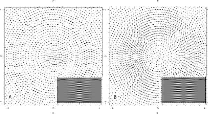
Figure 7: 8 $\times$ 8 $\mu$m cross sections of modes of a conducting cavity near maximum amplitude ($z=0.25$). $k_{\text{A}}=7.89285$ and $k_{\text{B}}=7.89290$. The inset plots show $\text{Re}E_{x}$ in the $x$-$z$ plane with horizontal and vertical tick marks every 1 $\mu$m.

Figure 7 shows the cross sections of two near-degenerate $m=1$ modes found for a conducting cavity. Here $z_{1}=z_{e}=0$ and M2 is spherical with radius $R_{s}=70$ but is centered at $z=-59.5$ instead of the origin, so that $R=10.5$. The paraxial parameter $h$ is at least as small as 0.1 (see the side views in the inset plots). Mode A corresponds very well to the pure $\text{LG}_{1}^{0}\bigl{(}\begin{smallmatrix}1\\ \imath\end{smallmatrix}\bigr{)}$ mode, while mode B corresponds very well to the pure $\text{LG}_{0}^{2}\bigl{(}\begin{smallmatrix}1\\ -\imath\end{smallmatrix}\bigr{)}$ mode. These are mixable modes, as indicated in Table 1, and the conducting cavity has “chosen” essentially zero mixing. Note that mode B would have zero overlap with an incident fundamental Gaussian beam centered on the $z$ axis, while mode A would have nonzero overlap.

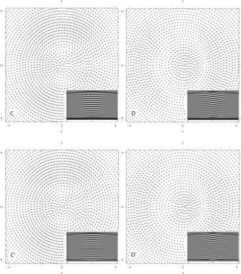
Figure 8: Cross sections of true modes (C and D) of a cavity with stack II near maximum amplitude ($z=0.05$), and constructed modes (C${}^{{}^{\prime}}$ and D${}^{{}^{\prime}}$) near their maximum amplitude ($z=0.25$). The constructed cross sections are nearly identical to the true cross section. $k_{\text{C}}=7.74685-\imath 0.00005415$, $k_{\text{D}}=7.74680-\imath 0.00005516$, and the constructed modes are plotted with $k_{\text{C}^{{}^{\prime}}/\text{D}^{{}^{\prime}}}=7.8929$, the average of $k_{\text{A}}$ and $k_{\text{B}}$. The inset plots show $\text{Re}E_{x}$ in the $x$-$z$ plane. The stack parameters are $N_{s}=22$ and $k_{s}=7.746814$.

Pictures C and D in Figure 8 are cross sections of near-degenerate $m=1$ modes for a cavity with stack II. To show that the transverse part of these modes are mixtures of A and B, we have added and subtracted the solution vectors $\bm{y}_{\text{A}}$ and $\bm{y}_{\text{B}}$ to create the new (non-solution) vectors:

$$\bm{y}_{\text{C}^{{}^{\prime}}}=\bm{y}_{\text{A}}+\eta\bm{y}_{\text{B}}, \bm{y}_{\text{D}^{{}^{\prime}}}=\bm{y}_{\text{A}}-(0.225)\eta\bm{y}_{\text{B}},$$ (86)

and have plotted these fields (C${}^{{}^{\prime}}$ and D${}^{{}^{\prime}}$) using $k=(k_{\text{A}}+k_{\text{B}})/2$. (The scaling factor $\eta$, here $\approx 0.07$, is unphysical and related to the effect of the seed equation on overall amplitude.) Comparing C${}^{{}^{\prime}}$ and D${}^{{}^{\prime}}$ with C and D shows that we have reconstructed the mode cross sections quite well (up to a constant factor). Modes C and D are not pure Hermite-Gaussian (HG) modes, but their resemblance to the $\text{HG}_{02}$ and $\text{HG}_{20}$ modes is not an accident. Mode conversion formulas in Ref. [15] show that $\text{LG}_{0}^{2}$ is made of the $\text{HG}_{02}$, $\text{HG}_{11}$, and $\text{HG}_{20}$ modes while $\text{LG}_{1}^{0}$ contains only $\text{HG}_{02}$ and $\text{HG}_{20}$. Note that both modes C and D would couple to a centered fundamental Gaussian beam.

An interesting property of the mixed modes C and D is that their general forms appear to be persistent as $h$ is varied, provided that the paraxial approximation remains sufficiently applicable. Furthermore, we do not have to be particularly careful about setting $\lambda_{s}$ to correspond very closely to $2\pi/\text{Re}k$. The modes shown in Figure 9 are not nearly as paraxial as the C and D modes. Here $k_{s}=8.1600$ which is not close to the $k$ values of the modes. Furthermore, stack I was used which is missing the spacer layer of stack II. Nevertheless the modes of Fig. 9 bear a strong resemblance to the more carefully picked C and D modes.

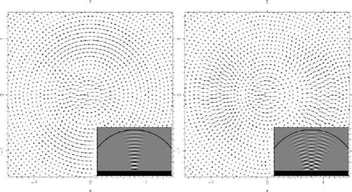
Figure 9: Cross sections of neighboring, poorly paraxial modes near maximum amplitude ($z=1.33$). M2 is spherical and origin-centered with $R=10$. M1 is stack I with $N_{s}=20$, $k_{s}=8.1600$, and $z_{1}=z_{e}=1.0$. The mode on the left has $k=8.51160-\imath 0.0002491$ and the mode on the right has $k=8.51540-\imath 0.0003184$.

5.3 Modes with $m\neq 1$

The $m=0$ modes may be circularly polarized, such as the paraxial $m=0$ modes of Table 1. The more interesting polarization, perhaps, is the $m=0$ analogue of $x$ and $y$ polarization: radial and azimuthal polarization. The mode shown in Fig. 10 is radially polarized, although it is impossible to tell this from the plots because the left and right circularly polarized modes are radial (identical to the plot) at $t=0$ and azimuthal (like a vortex) at $\omega t=\pi/2$. The radial or azimuthal polarizations are easier to obtain numerically than the right or left polarizations because radially (azimuthally) polarized modes have all of the $b_{l}$ ($a_{l}$) MB coefficients equal to zero and thus can be selected by the seed equation (see Appendix B).

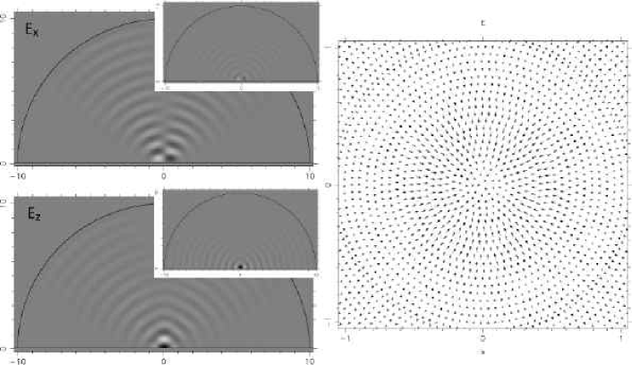
Figure 10: Tightly focused, radially polarized $m=0$ modes of a conducting cavity. The focusing has caused $E_{z}$ to be greater than the $E_{\rho}$. The spot size of the dominant $E_{z}$ field for such modes can be surprisingly small, as has recently been demonstrated experimentally by Dorn et al.[4] (for a focused beam with no cavity). Parameters of the non-inset cavity and mode are $R=10$, $z_{1}=0.05$, and $k=7.2481$ ($\lambda=0.867$). The cross section is at $z=0.3$. The insets show the mode after it was followed to the perfectly hemispherical $z_{1}=0$ cavity shape; here the mode has an even smaller central spot and $E_{z}\gg E_{\rho}$. We expect a hemispherical mode to have only a single nonzero MB coefficient and this was verified by the solution: $a_{1}=1.0$ and $|a_{l}|<1.1\times 10^{-7}$ for $l\neq 1$. The hemispherical mode has $k=7.2243$ ($\lambda=0.870$).

Figure 11 shows a $m=2$ mode that corresponds to the $\text{LG}_{1}^{1}\bigl{(}\begin{smallmatrix}1\\ \imath\end{smallmatrix}\bigr{)}$ mode from Gaussian theory. We also have completed the $N=2$ near-degenerate family by finding the $\text{LG}_{0}^{2}\bigl{(}\begin{smallmatrix}1\\ \imath\end{smallmatrix}\bigr{)}$ $(m=3)$ mode for both the cavity used in Fig. 7 ($k=7.8926\approx k_{A}\approx k_{B}$) and the cavity used in Fig. 8 ($k=7.7466-\imath 0.00005466\approx k_{C}\approx k_{D}$). The cross sections of this mode for the two cavities, which are not shown to conserve space, appear identical, as predicted by the absence of a $m=+3$ near-degenerate partner for this mode (Table 1).

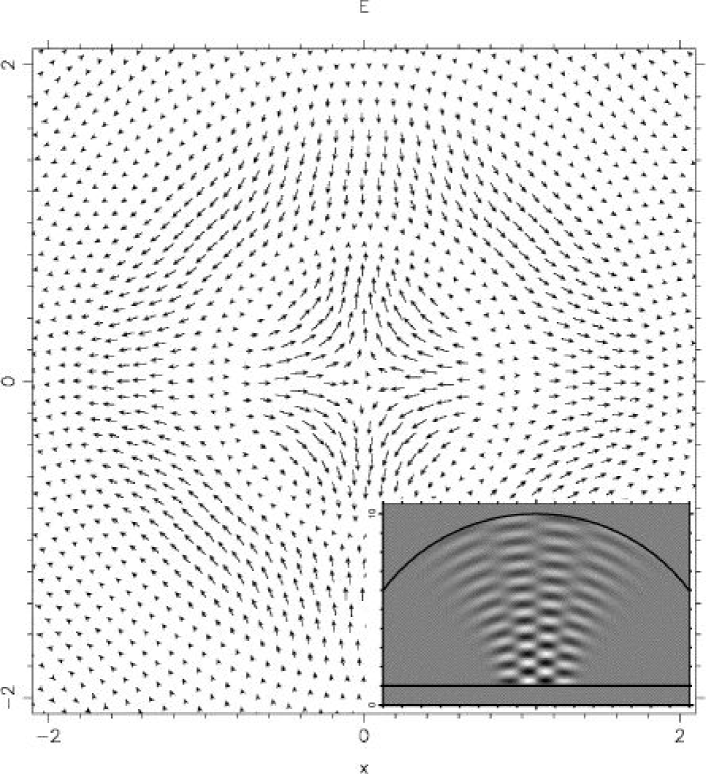
Figure 11: A $m=2$ mode for a conducting cavity ($k=7.885463$). M2 is spherical and origin-centered with $R=10$. M1 is a conductor; $z_{1}=1.0$. The inset shows $\text{Re}E_{x}$ in the $x$-$z$ plane.

5.4 $N_{\text{dirs}}$ and $l_{\text{max}}$: Comparing the Two Primary Methods

The authors of this paper first implemented the more complicated two-basis method, believing that many more PWB coefficients than MB coefficients would be required to expand dome-shaped cavity fields. When the Bessel wave method was implemented as a check, it was discovered that the PWB works surprisingly well, with usable values of $N_{\text{dirs}}$ being of the same order of magnitude as usable values of $l_{\text{max}}$. The choice of seed equation, $N_{\text{dirs}}$ or $l_{\text{max}}$, and other parameters can both affect the depth and narrowness of the dips in the graph of $\Delta_{r}$ versus $\text{Re}k$. This makes it difficult to perform a comprehensive and conclusive comparison of the two methods.

One practical problem with the Bessel wave method is that its performance is sometimes quite sensitive to the value of $N_{\text{dirs}}$. In both methods, setting the number of basis function too high results in a failure to solve for $\bm{y_{\text{best}}}$; the program acts as if $A\bm{y}=\bm{b}$ were underdetermined, even though the number of equations is several times the number of unknowns. When increasing $l_{\text{max}}$ or $N_{\text{dirs}}$ toward its problematic value, the $\Delta_{r}$ values for all $k$ dramatically decrease, sharply lowering the contrast needed to locate the eigenvalues of $k$. The solutions that are found begin to attempt to set the field to zero in the entire cavity region, with some regions of layer 0 outside the cavity having field intensities that are orders of magnitude larger than the field inside the cavity. In our experience this problem has not occurred in the two-basis method for $l_{\text{max}}$ near the semiclassical limit of $l$, $\text{Re}(kR)$, and thus has never been a practical annoyance. On the other hand, the problem can occur at surprisingly low values of $N_{\text{dirs}}$. Yet taking $N_{\text{dirs}}$ to be too low can often cause solutions to simply not be found: dips in the graph of $\Delta_{r}$ vs. $\text{Re}k$ can simply disappear. The window of good values of $N_{\text{dirs}}$ can be at least as narrow as $N_{\text{dirs}}/10$. The window of good $l_{\text{max}}$ values for the MB seems to be much wider (for many modes, it is sufficient to take $l_{\text{max}}$ to be half of $\text{Re}(kR)$ or less). In this respect, the two-basis method is easier to use than the Bessel wave method.

On the other hand, there were situations when a scan of $\Delta_{r}$ versus $\text{Re}k$ with the Bessel wave method revealed a mode that was skipped in the same scan with the two-basis method, due to the narrowness of the dip feature. To the best of our recollection, we have always been able to find a mode by both methods if we have made an effort to search for it.

A direct comparison of the methods by looking at the solution plots rarely reveals field value differences greater than 1% of the maximum value when the modes are restricted to those that do not have a large high-angle component. The eigenvalues of $k$ located by the two methods are usually quite close. Here we show one case in which there is a small but visible difference between the mode plots for the Bessel wave method and the two-basis method.

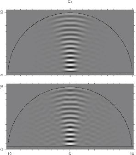
Figure 12: Top: Solution obtained with Bessel wave method. $k=8.57073-\imath 0.05857$; $\Delta_{n}=2.8\times 10^{-5}$, $N_{\text{dirs}}=30$; $\alpha_{k}^{(0)}$ distribution is uniform in $\Delta(\sin\alpha_{k}^{(0)})$, not $\Delta(\alpha_{k}^{(0)})$. Bottom: Solution obtained with two-basis method. $k=8.57086-\imath 0.05900$; $\Delta_{n}=2.9\times 10^{-5}$; $l_{\text{max}}=86$. The field in layer X is not plotted.

Figure 12 shows $E_{x}$ in the $x$-$z$ plane for a mode in a cavity with $n_{0}=1.0$ and $n_{X}=0.5$ and no stack layers at all. This situation is meant to model a dielectric-filled dome cavity surrounded by air. (Our program assumes that layer 0 is free space ($n_{0}=1$), so we have set $n_{X}<n_{0}$ to achieve this effect.) Here M2 is spherical and centered at the origin with $R=10$ and $z_{e}=z_{1}=0.5$. The reason for the disagreement between the two methods for this case is not known. This was the only low finesse cavity we have tried, as well as being the only cavity with a “high” index of refraction in layer 0. Another unusual property of this mode solution, which looks similar to a fundamental Gaussian, is that its electric field in the $x$-$y$ plane actually spirals: its instantaneous linear direction rotates with $z$ as well as with $t$. The other modes we show throughout the demonstrations section give extremely good agreement between the two primary methods.

In our implementation, computation time to set up and solve $A\bm{y}=\bm{b}$ is of the same order for the Bessel wave method and the two-basis method (with variant 1). For the large cavity shown in Fig. ​3, the Bessel wave method took about 10 s with $N_{\text{dirs}}=100$ and about 600 locations chosen on M2. Variant 1 with $l_{\text{max}}=200$, 600 M2 locations, and 600 uniformly spaced $\alpha_{k}^{(0)}$, took about 15 s. For comparison, Variant 2 took about 2 hours (achieving a $10^{-6}$ relative accuracy for each $\alpha_{k}^{(0)}$ integral).

5.5 Almost-Real MB Coefficients

When M1 is a conductor we find that the imaginary parts of $a_{l}$ and $b_{l}$ are essentially zero. Furthermore, we often find that for dielectric M1 mirrors, the imaginary parts of $a_{l}$ and $b_{l}$ are one or more orders of magnitude smaller than their real parts. We show one way in which this tendency simplifies the interpretation of mode polarization in Appendix B.

There is a an argument that suggests that $a_{l}$ and $b_{l}$ should be real for a conducting cavity. A conducting cavity has a real eigenvalues, $k$, and real reflection functions, $r_{s/p}=-1$. It is not difficult to see that for real $k$ the three types of M2 equations, $E_{\phi}=0$, $E_{\parallel}=0$, and $H_{\perp}=0$, can be satisfied with real $a_{l}$ and $b_{l}$. The seed equation of course can also be chosen so that it can be satisfied by real variables. The M1 equations, because of the complex nature of $\bar{r}_{s/p}=r_{s/p}\exp(-\imath 2z_{1}kn_{0}\cos\alpha_{k}^{(0)})$ when $z_{1}\neq 0$, are not obviously satisfied by real $a_{l}$ and $b_{l}$. However, for a conducting cavity, the M1 boundary condition can be given as a real space boundary condition (like M2) instead of a Fourier space boundary condition. In this case, locations on M1 are chosen just as they are on M2. The same argument that the M2 equations can be satisfied by real $a_{l}$ and $b_{l}$ now applies. Thus the M1 boundary condition for a conducting cavity should not, in any basis, force $a_{l}$ and $b_{l}$ to be complex.

6 Conclusions

The two methods presented in this communication have proved to be useful tools for modeling small optical dome-shaped cavities. As yet we have no general verdict on which method is best. Overall, it was quite helpful to have both methods available for finding all of the modes. Once a mode was found, agreement of both eigenvalue and eigenmode between the two methods was quite good.

The primary advantage of both of these methods is the treatment of the dielectric stack through its transfer matrices. First of all, including the dielectric stack in the model is essential to obtain a number of qualitative features of the modes. A model with a mirror of constant phase shift is inadequate, except in special cases such as the fundamental Gaussian mode in its paraxial regime. In addition, including the stack in the model allows one to calculate the field inside the stack, which may be the location of interest for the engineer of an optical device. Secondly, the use of the transfer matrices is the most natural way to include a dielectric stack that is of large lateral extent compared to the wavelength. The only alternative that we know of would involve a separate basis for each stack layer, resulting in an increase of both dimensions of the matrix $A$ by about $N$ times, where $N$ is the number of stack layers.

Another advantage of the methods we have presented is their speed. Each point in Fig. 5, which was generated in a few hours or less, required $A\bm{y}=\bm{b}$ to be constructed and solved 20–60 times for a cavity with $R\approx 50\lambda$. The combination of using a basis expansion method, taking advantage of cylindrical symmetry, using one basis set for all the layers, avoiding numerical integrals, and using C++ inline functions for complex arithmetic has resulted in a fast implementation.

Several “stack-induced” effects that we have demonstrated here will be more thoroughly treated in a separate publication. The splitting of the fundamental Gaussian (and other Gaussian modes) into a non-axisymmetric “V” shape may be of practical interest to workers who wish to achieve a tight focus. The $m=0$ modes, which have the greatest potential for tight focusing, are also of interest. The ability to analyze the persistent stack-induced mixing is a result that stands in its own right. This stack effect persists arbitrarily far into the paraxial limit; it exists as long as the resonance widths of both the cavity and the laser source are smaller than the splitting of the near-degenerate pair. This effect should exist for a wide range of cavity lengths, and is of interest to anyone engineering higher-order Gaussian modes.

Perhaps the greatest limitation to the practical application of our methods is its rigid treatment of the curved mirror as a conductor. As mentioned in the Introduction, it is reasonable to expect highly focused modes, such as those shown in Figs. 3, 6 and 10, to undergo little change when the curved conducting mirror is exchanged for a dielectric one (with an appropriate change of mirror radius by $-\lambda/4<\delta<\lambda/4$ to account for a phase shift). This is because the local wave fronts are primarily perpendicular to the curved mirror for such modes (imagine a Wigner function evaluated at the surface of M2). For paraxial geometries such as those in our discussion of stack-induced mixing, this argument says nothing about how replacing M2 with a curved dielectric stack will affect the modes. A pursuit of this question may require a more brute force approach.

Despite all limitations, we find our methods to be extremely versatile and powerful (fast and allowing for relatively large cavities). The full vector electromagnetic field is used. Exactly degenerate modes can be separated. The shape of the curved mirror is arbitrary and we have implemented parabolic shapes as well as spherical shapes with no difficulties. A first-try scan of $\Delta_{r}$ versus $\text{Re}k$ using either method with a non-contrived seed equation will locate the vast majority of modes that exist. Reasonable results are obtained when the interior of the cavity is a dielectric. Hopefully, the explicit development of the two methods given here can benefit a number of workers in optics-related fields.

Note Added in Proof

We note that we have not found significant stack-induced effects (the V mode of Section 5.1 and the mixing of Section 5.2) for a “standard” quarter-wave dielectric stack which has design ABAB$\ldots$AB with front surface A and $n_{A}>n_{B}$. If $n_{A}<n_{B}$, we do find both types of stack-induced effects. The standard ($n_{A}>n_{B}$) quarter-wave layer structure exhibits less variation in $\arg(r_{s/p}(\alpha_{k}))$ than our mirrors (cf. Fig. 15), and therefore behaves much like a perfect conductor except at high angles of incidence. The methods presented here, which model the curved dome mirror (M2) as a conductor, should therefore carry over to standard dielectric M2 mirrors. The planar mirror will in general have a “functional” layer design, leading to the stack-induced effects reported above.

Appendix A Further Explanations and Limitations of the Model

A.1 Exclusion of High-Angle Plane Waves

As mentioned in the Introduction, in the usual application of a basis expansion method, the field is expanded in each dielectric region separately and henceforth each region gets its own complete basis and its own set of coefficients. However, our methods, when “cast” into the PWB, use a single set of plane waves, complete in layer 0, which are propagated down into the other layers via the transfer matrices. There are several advantages to this approach. The Bessel wave method becomes simpler, as there are far fewer unknowns. This approach is also ideal for incorporating the use of the MB for layer 0, as in the two-basis method, although a straightforward use of the MB for layer 0 and a separate PWB for each layer $q$, $q>0$, could be implemented.

One drawback to our approach is that certain high-angle or evanescent plane waves are not included. No plane wave basis vectors are allowed for which $n_{q}\sin\theta_{k}^{(q)}>n_{0}$. If the true quasimode expansion in any layer has significant weight for these high-angle or evanescent waves, the calculated solution of the field could be erroneous.

Probably the best way to determine whether or not such intrinsic error is present at a significant level is to look at the plane wave distribution in layer 0 (using (58) or (82) to get this if one is using the two-basis method) and to see whether the distribution dies off as $\alpha_{k}^{(0)}$ approaches $\pi/2$. If it does, the solution should be reasonably error free.

We note here that Berry [16] has shown how evanescent waves, in a finite region near the origin, can be expressed in the PWB (using plane waves with real-valued directions, as usual). Thus the fact that no evanescent waves are included in layer 0 may not be a problem in itself for depicting the field in layer 0.

A.2 The Hat Brim

A.2.1 The infinitesimal hat brim

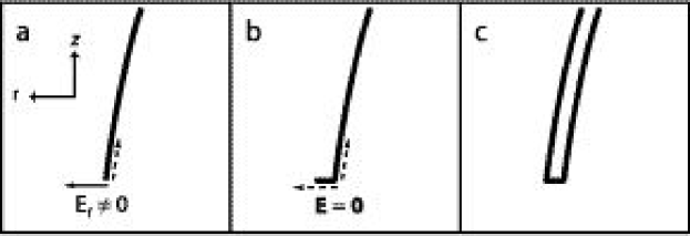
Figure 13: Modeling the edge of the dome.

For the vector field solution, a tiny hat brim must be added to M2 to correctly model a conducting edge. Figure 13 shows a cross section of the edge of M2 for increasingly better approximations of a real conducting mirror. In (a), $E_{\rho}$ can be nonzero at the edge, which is unphysical. In (b), a small hat brim has been added and $\bm{E}=\bm{0}$ at the inside edge, as it should be. In (c), locations are chosen on a (closed) conductor with finite thickness. As the thickness of M2 becomes insignificant compared to $\lambda$, model (b) should approximate model (c) arbitrarily closely. Usually 2–10 locations are chosen on the hat brim (the density of course is much greater on the hat brim than on the dome). We have taken $\omega_{b}\approx 0.0001\mu\text{m}$ for our demonstrations.

A.2.2 The infinite hat brim and the 1-D half-plane cavity

The way in which our model includes the interior of the cavity and the entire $z>z_{1}$ half-plane in a single region, layer 0, is somewhat unorthodox. We believe our method produces the correct field in a finite region surrounding the cavity, but not at $z\rightarrow\infty$.

A somewhat less strange model is obtained if one imagines an infinite hat brim. The upper half-plane is then no longer in the problem. Layer 0 still extends infinitely in $\rho$ as do the other layers, but the vertical confinement makes it easier to see that this is an eigenproblem and not a scattering problem. Unfortunately our implementation does not allow an infinite hat brim (unless M1 is a conductor and $z_{e}=z_{1}$, for which the hat brim condition is already set in the M1 equations). At least for some solutions, taking $w_{b}\approx R$ and giving the hat brim roughly the same number of locations as the dome, produces no visible changes in the mode structure (from the solution obtained with a tiny hat brim). The mode shown in Fig. ​3 is one of these.

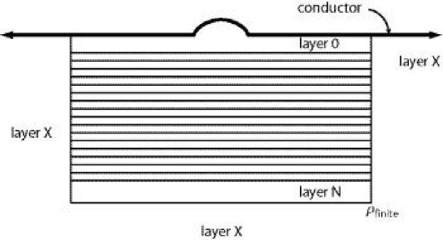
Figure 14: Including the sides of the stack at radius $\rho_{\text{finite}}$.

If we allow that some solutions are not affected by the value of $w_{b}$, we can take the infinite hat brim more seriously. The problem becomes similar in some respects to the 1-D half-plane problem, in which $x<0$ is a conductor, $x>L$ has a constant refractive index, and the $[0,L]$ region is segmented into several 1-D dielectric layers. The solutions of the 1-D problem form a set of quasimodes, (or quasinormal modes), which are complete in $[0,L]$ and obey an orthogonality condition on the same interval. The conditions for completeness, and the characterization of the incompleteness of the quasinormal mode for problems which do not meet the completeness conditions, are discussed in Ching et al. [17] and Leung et al. [18]. The model with the infinite hat brim does not rigorously meet the the completeness condition (for 3-D cavity resonators). We note that it appears from the references mentioned above that the situation depicted in Fig. ​14 would meet the completeness condition, with the quasinormal modes being complete in layers $0$–$N$. We do not attempt to resolve this further, as the use of our mode solutions as a basis for time-dependent problems is beyond the scope of what we have been trying to accomplish.

Appendix B Negative $m$ Modes and Sine and Cosine Modes

The cylindrical symmetry group consists of $\phi$-rotations and reflections about the $x$-$z$ or $y$-$z$ planes. For solutions with a fixed, nonzero $m$, rotations are equivalent to multiplying the field by a complex phase, which is of course equivalent to a translation in time. (This means that, when looking at any cross section plot in Section 5 for a fixed $m\neq 0$, the time evolution can be realized by simply rotating the figure: counter-clockwise for $m>0$ and clockwise for $m<0$.) Thus we say that for $m\neq 0$, reflections generate a new solution but rotations do not. (If we were considering the sine and cosine modes discussed later in the section, instead of the $\pm m$ modes, we would say that a $\pi/(2m)$ rotation generates a new solution but a reflection does not.) Hence the symmetry of the cavity causes modes to come in truly degenerate pairs. It can be shown that a reflection is equivalent to taking $m$ to $-m$ (up to a $\pi$ rotation). For $m\neq 0$, general complex linear superpositions of the $\pm m$ pair of modes are equivalent to arbitrary complex superpositions of any number of $\phi$-rotations, reflections, and combinations of these acting on a single $+m$ mode. We note that since our methods solve $\bm{y}$ for a fixed $m$, we are able to separate the $\pm m$ pairs.

The $m=0$ modes also come in degenerate pairs, but the interrelation can be more complicated than a reflection. The $m=0$ pairs can be separated easily in the two-basis method by choosing a seed equation that contains only $a_{l}$ or only $b_{l}$ coefficients, since the M1 and M2 equations do not couple $a_{l}$ and $b_{l}$ coefficients if $m=0$. Thus all of the true (non-accidental), exact (not obtained only in a limit, such as the paraxial limit) degeneracies that exist can be separated.

In constructing the M1 and M2 equations, it is easiest to write code that assumes that $m\geq 0$. For presentations and movies, it is nice to be able to plot both $+m$ and $-m$ solutions, as well as the linear combinations adding and subtracting these modes. All four of these modes can be plotted from a solution $\bm{y}_{+m}$ that has been been found using the positive azimuthal quantum number $+m$. Here we briefly discuss how to do this (for $m\neq 0$).

B.1 Plotting with -m

To plot the $-m$ modes, we use simple rules, allowed by the M1 and M2 equations, to create a new solution vector $\bm{y}_{-m}$ from the solution $\bm{y}_{+m}$. To obtain the field, the new coefficients from $\bm{y}_{-m}$ are simply inserted into the various expansion (or basis conversion) equations from Sections 3 and 4, using $(-m)$ as the “$m$” argument in these equations. (All of these equations work for negative values of their $m$ argument.) The relations $Y_{l,-m}=(-1)^{m}Y_{lm}^{*}$, $J_{-m}=(-1)^{m}J_{m}$, $f_{l,-m}=(-1)^{m}f_{lm}$, and $g_{l,-m}=-(-1)^{m}g_{lm}$ are useful. The rules for the new solution vectors are given in Table 2. (There is a certain arbitrariness to these rules, since $(\alpha\bm{y})$, with $\alpha$ being an arbitrary constant, satisfies the M1 and M2 equations.)

Table 2: Rules for taking $\bm{y}_{+m}\rightarrow\bm{y}_{-m}$.

	PWB	MB
scalar:	$\psi_{u,-m}=(-1)^{m}\psi_{u,+m}$	$c_{l,-m}=c_{l,+m}$
vector:	$S_{u/d,-m}=-(-1)^{m}S_{u/d,+m}$	$a_{l,-m}=a_{l,+m}$
	$P_{u/d,-m}=(-1)^{m}P_{u/d,+m}$	$b_{l,-m}=-b_{l,+m}$

B.2 Plotting cosine and sine modes

We can define the “cosine” and “sine” modes as $X_{(c)}\equiv(X_{(+m)}+(-1)^{m}X_{(-m)})/2$, and $X_{(s)}\equiv(X_{(+m)}-(-1)^{m}X_{(-m)})/2$, where $X$ stands for $\psi$, $\bm{E}$, or $\bm{H}$. By adding explicit expansion expressions for the $+m$ and $-m$ modes, one can obtain expressions for $X_{(c)}$ and $X_{(s)}$. For example, using (61), (62), and the above rules one finds that

$$\bm{E}_{(c)}^{(0)}(\bm{x},t)=e^{-\imath\omega t}\sum_{l}\Biggl{\{}\hat{\bm{r}}\biggl{[}a_{l}\frac{-l(l+1)}{kn_{0}r}j_{l}\text{Re}Y_{lm}\biggr{]}\\ +\hat{\bm{\theta}}\biggl{[}a_{l}\frac{-1}{kn_{0}r}\frac{\partial}{\partial r}(rj_{l})\frac{\partial}{\partial\theta}(\text{Re}Y_{lm})+b_{l}\frac{-m}{\sin\theta}j_{l}\text{Re}Y_{lm}\biggr{]}\\ +\hat{\bm{\phi}}\biggl{[}a_{l}\frac{m}{kn_{0}r\sin\theta}\frac{\partial}{\partial r}(rj_{l})\text{Im}Y_{lm}+b_{l}j_{l}\frac{\partial}{\partial\theta}(\text{Im}Y_{lm})\biggr{]}\Biggr{\}},$$ (87)

where $a_{l}$ and $b_{l}$ come from the original $\bm{y}_{+m}$. When $a_{l}$ and $b_{l}$ are predominately real (see Section 5.5), we can see from the above equation that the real-valued physical fields $E_{\rho}$ and $E_{z}$ are proportional to $\cos m\phi\cos\omega t$ while $E_{\phi}$ is proportional to $\sin m\phi\cos\omega t$. (The cosine time-dependence of $\bm{E}$ is why we call this the cosine mode.) Thus for the cosine mode with $|m|=1$, the transverse portion of $\bm{E}$ has an average linear polarization along the $x$ axis (note $\langle E_{y}\rangle_{\phi}=0\;\forall t$), as opposed to the average circular polarization the $m=\pm 1$ modes would have. (For the $m=+1$ mode, $\langle\bm{E\cdot}\hat{\bm{q}}\rangle_{\phi}=0\;\forall t$ where $\hat{\bm{q}}\equiv-\hat{\bm{x}}\sin\omega t+\hat{\bm{y}}\cos\omega t$.) Due to their separating of time and $\phi$-dependence for the physical fields, the sine and cosine modes are very useful final forms of the field (when $a_{l}$ and $b_{l}$ are predominately real).

Appendix C Stacks used in Section 5

Stacks I and II are similar to Al_1-xGa_xAs–AlAs stacks that Raymer has used experimentally [8]. Figure 15 shows the reflection phases for stack II. The stack parameters that are varied in our demonstrations are $N_{s}$ and $k_{s}\equiv 2\pi/\lambda_{s}$. The meaning of these parameters can be inferred from the stack definitions below. The normal reflection coefficient for stack II with $N_{s}=20$ is $|r_{s/p}(\alpha_{k}=0)|=0.9964$. For $N_{s}=22$, $|r_{s/p}|=0.9981$.

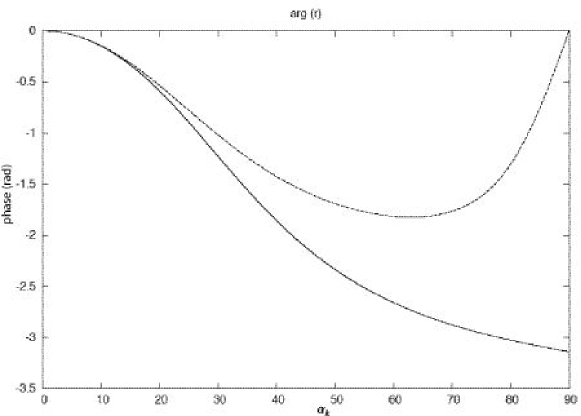
Figure 15: Plane wave reflection phases (rad.) of stack II ($N_{s}=20$) as a function of $\alpha_{k}$ (deg.). The solid (dashed) line is for s (p) polarization. The wavelength of the plane wave, $\lambda_{\text{test}}$, is set at $\lambda_{s}$. The graph for stack I is similar.

Stack I: $n_{0}=n_{X}=1$; $n_{1}=n_{3}=\ldots=n_{(2N_{s}-1)}=3.003$; $n_{2}=n_{4}=\ldots=n_{(2N_{s})}=3.51695$. Layers 1–$(2N_{s})$ are quarter-wave layers (optical thickness $=\lambda_{s}/4$).

Stack II: $n_{0}=n_{X}=1$; $n_{1}=n_{3}=\ldots=n_{(2N_{s}+1)}=3.51695$; $n_{2}=n_{4}=\ldots=n_{(2N_{s})}=3.003$. Layers 2–$(2N_{s}+1)$ are quarter-wave layers. Layer 1 is a spacer layer that has optical thickness $1\lambda_{s}$.

References

• [1] P. L. Greene and D. G. Hall, “Focal shift in vector beams”, Opt. Expr. $\bm{4}$ (1999) 411.
• [2] P. L. Greene and D. G. Hall, “Properties and diffraction of vector Bessel-Gauss beams”, J. Opt. Soc. Am. A $\bm{15}$ (1998) 3020.
• [3] C. J. R. Sheppard and P. Török, “Efficient calculation of electromagnetic diffraction in optical systems using a multipole expansion”, J. Mod. Opt. $\bm{44}$ (1997) 803.
• [4] R. Dorn, S. Quabis, and G. Leuchs, “Smaller, sharper focus for a radially polarized light beam”, Phys. Rev. Lett. $\bm{91}$ (2003) 233901.
• [5] J. U. Nöckel, G. Bourdon, E. Le Ru, R. Adams, I. Robert, J-M. Moison, I. Abram, “Mode structure and ray dynamics of a parabolic dome microcavity”, Phys. Rev. E 62 (2000) 8677.
• [6] J.U. Nöckel and R.K. Chang, ”2-d Microcavities: Theory and Experiments”, in Cavity-Enhanced Spectroscopies, Roger D. van Zee and John P. Looney, eds. (Experimental Methods in the Physical Sciences 40), Academic Press, San Diego (2002), 185–226.
• [7] A. E. Siegman, Lasers, University Science Books, Sausalito, CA, 1986, pp. 626–97, 744–76.
• [8] M. G. Raymer (colloquium, University of Oregon, 4/24/03, and private communication).
• [9] M. Aziz, J. Pfeiffer, and P. Meissner, “Modal Behaviour of Passive, Stable Microcavities”, Phys. Stat. Sol. (a) 188 (2001) 979.
• [10] J. D. Jackson, Classical Electrodynamics, Third Edition, John Wiley & Sons, Inc., New York, 1999, pp. 107–10, 113–4, 426–32, 471–73.
• [11] P. Yeh, Optical waves in layered media, Wiley, New York, 1988, pp. 60–64, 102–15.
• [12] W. H. Press, S. A. Teukolsky, W. T. Vetterling, B. P. Flannery, Numerical Recipes in C: The Art of Scientific Computing, Second Edition, Cambridge University Press, Cambridge, 1992, pp. 59–70, 359–62.
• [13] G. B. Arfken and H. J. Weber, Mathematical Methods for Physicists, Fifth Edition, Harcourt Academic Press, San Diego, 2001, p. 767.
• [14] G. Videen, “Light Scattering from a particle on or near a perfectly conducting surface”, Optics Communications 115 (1995) 1.
• [15] M. W. Beijersbergen, L. Allen, H. E. L. O. van der Veen, and J. P. Woerdman, "Astigmatic laser mode converters and transfer of orbital angular momentum". Optics Communications 96 (1993) 123.
• [16] M. V. Berry, “Evanescent and real waves in quantum billiards and Gaussian beams”, J. Phys. A: Math. Gen. 27 (1994) L391.
• [17] E. S. Ching, P. T. Leung, A. Maassen van den Brink, W. M. Suen, S. S. Tong, K. Young, “Quasinormal-mode expansion for waves in open systems”, Rev. Mod. Phys. 70 (1998) 1545.
• [18] P. T. Leung, S. Y. Liu, and K. Young, “Completeness and orthogonality of quasinormal modes in leaky optical cavities”, Phys. Rev. A 49 (1994) 3057.