The photomultiplier tube testing facility for the Borexino experiment at LNGS.

Abstract

A facility to test the photomultiplier tubes (PMTs) for the solar neutrino detector Borexino was built at the Gran Sasso laboratory. Using the facility 2200 PMTs with optimal characteristics were selected from the 2350 delivered from the manufacturer.

The details of the hardware used are presented.

A.Brigatti, A.Ianni, P.Lombardi, G.Ranucci³, and O.Smirnov

1 Introduction

1.1 The Borexino experiment

Borexino, a large scale liquid scintillator detector under construction at the Gran Sasso underground laboratory (LNGS), is a low energy solar neutrino detector designed for ${}^{7}Be$-neutrinos registering[1]. The scintillation photons produced by the recoil electrons are detected by 2200 photoelectron multiplier tubes (PMTs) placed around a transparent inner vessel containing a scintillating mixture. In addition 200 PMTs are used in the external Cherenkov light muon veto system. The Borexino design is described in detail elsewhere [2].

The Monte Carlo simulation of the Borexino detector predict that the mean number of photoelectrons (p.e.) registered by one PMT will be in the region $0.02-2.0$ for an event with energy of 250-800 keV. The interaction point in the detector is reconstructed using the time information from PMTs. The position resolution depends therefor on the precision of measurement of the arrival time of a single photoelectron. The accurate energy measurement in its turn demands good single electron charge resolution. Hence, the PMTs should demonstrate a good single electron performance both for the amplitude and the timing response. Furthermore, in order to minimize the probability of the random triggers during the acquisition, the PMT should feature a low dark rate. Another parameter to be kept under control is the probability of the delayed trigger of the system which depends on the PMT afterpulsing rate (mainly ionic afterpulses). The overall required detector performances define the acceptable characteristics for the PMTs, which are summarized in table 1. After preliminary tests ([3, 4, 5, 6]), the ETL9351 with a large area photocathode (8”) has been chosen [7]. Because of very low radioactive background needed for the operation of the Borexino detector, very strict limits were set on the content of the radioactive impurities in the PMT constructive materials. All the PMT components were thoroughly examined for the content of the radioactive elements from the ${}^{238}U$ (design radiopurity of $<3\times 10^{-8}$ g/g) and ${}^{232}Th$ chains ($<1\times 10^{-8}$ g/g), and ${}^{40}K$ ($<2\times 10^{-5}$ g/g of natural $K$ content) in the glass of the PMT. The radioactivity measurements were performed with $Ge$ spectrometry at the Gran Sasso underground laboratory. The design radiopurities of all the PMTs components were achieved, the detailed report on the measurements can be found in [8].

Before installation all PMTs have been tested in the special facility. The procedure of the testing includes adjustment of the operating voltage in order to set the multiplier gain to $k=2\times 10^{7}$.

In August 2001 bulk testing of 2350 PMTs for the Borexino was completed, and 2000 PMTs with the best performances were selected for the installation in the Borexino detector. The high efficiency of the equipment permitted to complete PMT testing within 4 months.

Parameter	$f_{dark}$	$p/V$	$\sigma_{t}$	$p_{late}$	$p_{prep}$	$p_{a}$
	<20 Kcps	>1.25	<1.25 ns	<5%	<1%	<5%

Table 1: Acceptance characteristics of a PMT:

• dark rate (with a discriminator threshold set at 0.2 p.e. level);

• peak-to-valley ratio (the ratio of the peak value in the charge spectrum to the value at the valley between the low- amplitude pulses and the main peak);

• the rms of the Gaussian fitting the main peak in the transit time distribution;

• late pulsing in percent, estimated as the ratio of the events in the $[t_{0}+3\cdot\sigma_{t};100]$ ns range to the total number of the events registered in the 100 ns interval;

• prepulsing in percent, estimated as the ratio of the events in the $[\textrm{t}_{0}-20;t_{0}-3\cdot\sigma_{t}]$ ns range to the total number of the events;

• total amount of afterpulses following the single electron response in the time interval up to 12 $\mu s$ (measured in percent in respect to the amount of the main pulses).

1.2 8” PMT ETL9351 and its characteristics

Figure 1: The base used for the Borexino PMTs.

A PMT of this model has 12 dynodes with a total gain of $k=10^{7}$. The transit time spread of the single p.e. response is about $1$ ns. The PMT has a good energy resolution characterized by the peak-to-valley ratio. The manufacturer (Electron Tubes Limited ETL) guarantees a peak-to-valley ratio of 1.5.

The PMTs delivered are factory tested and the operational high voltage (HV) is specified by the manufacturer. Selective measurements of the PMTs at the specified voltage showed a high variance of the gain near its mean value of $k=(0.86\pm 0.25)\times 10^{7}$. Moreover, the high voltage divider used by ETL and the one used in Borexino are different. For these reasons the operational voltage was readjusted. The Borexino PMT divider is shown in Fig.1. The signal and the high voltage are carried on the same cable. The signal decoupler scheme is shown in Fig.2. For proper signal termination a 50$\Omega$ resistor R1 is included in the anode chain. The resistor decreases the signal amplitude by a factor of 2. The signal attenuation is compensated by the higher operating voltage. Thus actually, the high voltage is adjusted for each PMT in order to provide photoelectron multiplier gain $k=2\times 10^{7}$.

Figure 2: Signal decoupler used with the Borexino PMTs

2 The PMT test facility at LNGS

Several PMT test facilities were prepared in the past by collaborations planning to use big number of PMTs in their detectors, such as the IMB [9], CHOOZ [10] and SNO [11] experiments. Also for the Borexino experiment a special PMT test facility was prepared at the LNGS. The photomultipliers used in the prototype of the Borexino detector, the Counting Test Facility (CTF) [12], were tested with a simpler facility, described in [6]. The Borexino PMT test facility is placed in two adjacent rooms. In one room the electronics is mounted, while the other one is a dark room with 4 wooden tables designed to hold up to 64 PMTs. The tables are separated from each other by black shrouds, which shield the light reflected from the PMTs photocathode. Together with the acceptance tests, performance of the PMTs immersed in water was tested, in order to study the possible mechanical problems for PMTs to be mounted at the bottom part of the Borexino detector. For this purpose 3 pressurized Water Tanks (WT) were installed, each of the tanks can hold up to 20 PMTs. For the purpose of the long-term testing of the PMTs in conditions close to the ones of the Borexino detector a Two-Liquid Test Tank (TLTT) was designed and installed in the laboratory [13]. 48 PMTs are installed in the TLTT, with the base being in water and the bulb immersed in liquid scintillator. Actually, the TLTT test has now been running for more than 3 years, data is taken periodically in order to check the PMT signal degradation. Only two PMTs of the total 48 are found non-operational after these 3 years.

The overall test facility is therefore able to measure the characteristics of 172 PMTs if completely loaded. The electronics system consists of the high voltage supplies and the independent signal processing electronics. The high voltage supplies can provide high voltage to all PMT under test. In order to avoid unnecessary system duplication, only 32 electronics channels are used for the signal processing at the same time. The PMTs under test are grouped by no more than 32 in one group. The switching between the groups is performed by means of 8 analogical multiplexers, which provide control over 4 complete groups. Two groups of 32 PMTs each are connected to the 64 cables of the dark room. Another two groups can be connected interchanging the cables either to the 60 PMTs in the WTs (20 PMTs each), or to the 48 PMTs of the TLTT (24 PMT in each group). The tests with the TLTT are rare and the connection of the signal cables is performed manually.

The dark room is equipped with a system compensating the Earth’s magnetic field ([14]). The non-uniformity of the compensated field in the plane of the tables is no more than $10\%$. In the WTs and the TLTT the Earth Magnetic Field is not compensated.

The PMT characteristics are defined during a 8 hours run. The stability of the parameters is defined every 12-24 hours during longer runs.

2.1 The Earth magnetic field compensation system

Magnetic fields as weak as the Earth’s magnetic field (EMF, $\sim 40\mu T$) affect PMT performances and it turns out that tubes with linear focusing dynodes (as the Borexino 8" ETL9351) are most sensitive to magnetic influence when the field is parallel to the dynodes [5, 15].

In the area of the external Gran Sasso Laboratory the static EMF is about 35$\mu$T in the vertical direction, 25$\mu$T along the north-south direction and 8$\mu$T along the east-west direction. A daily change around 0.05$\mu$T was observed. Therefore, a compensation of the north-south and vertical components of the static EMF was needed; the component varying in time is negligible and can be left without compensation. Since the test facility tables occupy in total 2x2 m², a large compensated volume is needed. The EMF compensation system of the test facility is based on a system of rectangular coils; the choice is characterized by simple construction, easy access to the internal area, and by an excellent ratio of uniform field to coils volume [17]. Since the dark room is in iron-reinforced concrete building with dimensions of 5x5x3 m³ made of two sandwich-walls, one should expect spatial variations of the EMF over the useful volume. Therefore, the EMF was mapped inside the dark room. Moreover, in order to avoid any interference with the compensation system, the support structure for the phototubes has been manufactured with wood.

A number of various systems of rectangular and square coils was studied. A four square coils system (FCMS) as designed by R. Merritt and coworker [17] was chosen in order to compensate the crucial north-south component. In order to analyze the magnetic field created by the FCMS a master formula for a general rectangular coil was written as described in [14]. The field uniformity inside the coils system, $U$, was characterized by the field deviations with respect to the field at the center:

$$U=\arrowvert\frac{\overrightarrow{H}(x,y,z)-\overrightarrow{H}(0,0,0)}{\overrightarrow{H}(x,y,z)}\arrowvert.$$ (1)

where $\overrightarrow{H}(x,y,z)$ is the field at the point $(x,y,z)$ and $\overrightarrow{H}(0,0,0)$ is the field at the center of the system. The field $\overrightarrow{H}(0,0,0)$ was chosen to fully compensate the measured EMF at the dark room center. The coil currents were calculated on the basis of this value.

A FCMS with 2.84m coils side length was chosen to compensate the north-south component. Another system consisting of two square coils with 2.98 m side length and spacing equal to 1.4m was chosen to compensate the vertical component of the EMF. The effect of the finite cross section of the coils (66 mm²) was taken into account as described in [20], but the corrections were found to be negligible because of the huge coil sizes.

The useful volume for arranging the PMTs was defined determining the 10% deviation of the magnetic field from the mean value in a plane crossing the center of the coil system. All field components were treated independently. In Fig.3 is shown the coil system with it reference frame. The measurements confirmed a good uniformity of the EMF in a volume of 2x2x0.6 m³ lying in the xz plane. In Table 2 all the parameters of the six coil system are reported.

Table 2: Coil system parameters.

Four coil system (FCMS)
	inner coils	outer coils
side length	2.84m	2.84m
distance to the center	0.363m	1.434m
current	0.34 A	0.80 A
number of turns	47	47

Two coils system (square Helmholtz coils)
side length	2.98m
distance between the coils	1.4m
current	1.11 A
number of turns	50

The measurements of the EMF inside the dark room were performed with an analog Magnetoscope 1.608 by Foerster which is an intensity and gradient magnetic field sensor operating with a Foerster probe. The precision of the instrument is 3% for all the scales. Two sets of measurement were performed at the level of 146 and 129 cm from the ground. The results of measurement were reported in [21]. On the basis of the analysis of the field uniformity, the PMT support tables were placed in a suitable area (far away from the entrance door and the cables patch-panel). Measurements of the effect of movements of a big bridge crane located in vicinity of the dark room were performed as well [14].

The power supply for the 6 coil system inside the dark room (see Fig.3) is guaranteed by a single double Elind generator which is able to provide a stabilized current up to 0.01 A. Each coil consists of a wooden structure with three layers of copper-wire turns (see Table 2). Fig.4 and Fig.5 present the results of the final measurements after the coil installation.

Once the coil system was built and operating the measurements were performed in order to check the compensated field. The tables for the PMTs have in total 64 holes. The field at the center of each hole has been measured. Fig.6 shows the results of measurements with the compensated field. One can see that the developed coils system compensates the EMF at the level of 1.5 $\mu$T for the north-south component (FCMS), and 5 $\mu$T for the vertical component (non standard Helmholtz system of square coils). The value of 8.5 $\mu$T is measured for the non-compensated east-west component. The expected PMT signal degradation due to the residual EMF is less than 5% [5].

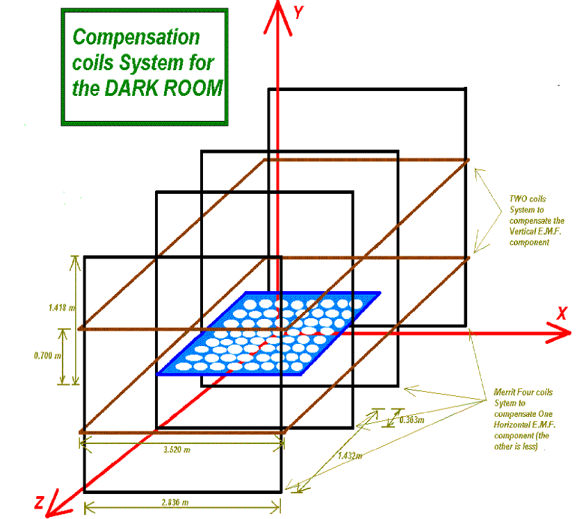
Figure 3: Coil system and reference frame.

Figure 4: Magnetic field measurements. See text for details.

Figure 5: Magnetic field measurements. See text for details.

Figure 6: Residual field measured at the center of each PMT position inside the dark room.

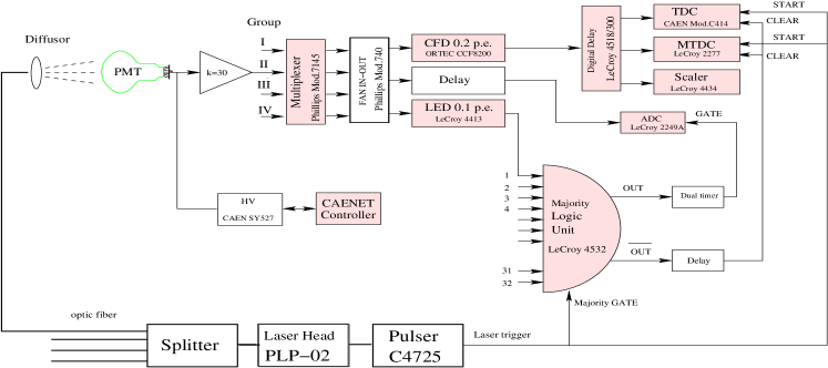
Figure 7: One channel of the electronics used in the measurements; a PMT of Group II is shown. CAMAC standard modules controlled (and/or read) by a personal computer via a CAEN C111 interface are shown in gray color.

2.2 Electronics

One channel of electronics (out of the total 32) of the test facility is presented in Fig.7. The system uses the modular CAMAC standard electronics and is connected to a personal computer by a CAEN C111 interface.

Figure 8: The schematic of the channel multiplexing

As it was already pointed out, the test system operates only on one of 4 groups of PMTs at the same time. The logic of the channels multiplexing is shown in Fig.8. The switch between the groups is performed writing the corresponding mask into the multiplexer internal register. The Quad linear FAN-IN/OUT (Philips Mod.740) is connected as analog signals summator. The signal is amplified before multiplexing in order to preserve the signal-to-noise ratio. After splitting the signals are processed by a LeCroy Mod.4413 Leading Edge Discriminator (LED) with a threshold set at the level of $0.05-0.10$ p.e., just above the level of the noise. If the PMT in the current channel is too noisy, the channel is disabled by writing the corresponding mask into the internal register of the LED, in such a way avoiding the influence of the elevated count rate in one channel on others. The signals formed by the LED are fed into the LeCroy Mod.4532 Majority Logic Unit (MALU). If at least one signal from the total 32 occurs inside the external gate, the output signal is generated and the LAM signal is activated by the MALU. The laser trigger is used as the majority external gate.

The Ortec Mod.CCF8200 Constant Fraction Discriminator (CCF) was used for the measurements of the timing characteristics with the threshold set at the 0.2 p.e. level. The formed signals are delayed and split on the Digital Delay (LeCroy Mod.4518/300) and then fed into the CAEN Mod.C414 Time-to-Digital-Converter (TDC), the LeCroy Mod.2277 Multihit TDC (MTDC) and the Scaler (LeCroy Mod.4434). The original signal delayed on the Delay Line is fed into the LeCroy Mod.2249A Analog-to-Digital Converter (ADC). The ADC “gate” and the TDC/MTDC “start” signals are generated using the laser internal trigger, which has a negligible time jitter ($<100\>ps$) with respect to the light pulse.

The MALU is able to memorize the pattern of the hit channels. This information significantly increases the data processing rate. The read-out of the electronics is activated when the majority LAM signal is on. Otherwise, a hardware clear is forced 400 ns after the laser trigger, using the majority $\overline{OUT}$ signal.

Two modes of operation were used in our tests. In the first one, the system is triggered at the first trigger from the laser that occurs when the electronics is not busy processing the previous event. This was realized by connecting the last (32-nd) majority input to the external gate signal. This mode of operation has been used in the test of the PMTs. An example of the data acquired during a routine PMT test is presented in Fig.9.

Another mode of operation has been used during the HV tuning. In this case the 32-nd input of the MALU was disabled. The electronics read-out was activated as before by the MALU LAM signal, but for this time at least one signal from PMT over the LED threshold must be present to activate the MALU. In such a way the “cut” charge histograms have been acquired with a hardware threshold of about $5\%-10\%$ of the “typical” Single Photoelectron Response (SER) mean value.

The afterpulses are registered by the MTDC which is able to record in the internal register up to 16 sequential hits inside a 32 $\mu s$ window for each of its 32 channels. The laser repetition rate was tuned to 30 $\mu$s, so the peak corresponding to this time can be clearly seen at the afterpulses histogram. The intensity of this peak was used to monitor the intensity of the laser. The probability of two sequential nonzero PMT signals, in the assumption of the Poisson distribution of the number of detected photoelectrons, is given by:

$$\mu=-\ln(1-\frac{N_{2}}{N_{1}})\simeq\frac{N_{2}}{N_{1}},$$

for $\mu\ll 1$, where $N_{2}$ is number of events in the second peak and $N_{1}$- number of events in the first peak (or the total number of the system triggers in our case). The time of arrival of the first pulse was tuned to have it just after the MTDC start signal, so the MTDC counts the number of its triggers.

The high precision calibration of each electronics channel was performed before the measurements. Here calibration means the ADC response to a signal corresponding to 1 p.e. on the system input with the ADC pedestal subtracted (the PMT in this measurement was substituted by a precision charge generator LeCroy 1976). The position of the ADC pedestals are defined and checked during the run.

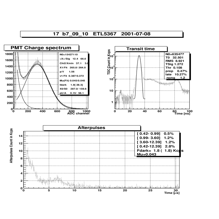
Figure 9: The characteristics of one of the PMTs under test: charge spectrum, single photoelectron transit time and afterpulses. The PMT charge response is measured in ADC channels (1024 ADC channels correspond to 256 pC).

2.3 High voltage supplies

Two types of high voltage supplies were used to provide HV to the PMTs. The CAEN mainframe mod. SY403, with 4 mod. A505 boards (3 kV, 200 $\mu$A) of 16 channels each, was used to provide HV for the PMTs in the dark room. This model has very low r.f. noise and provides the possibility to check the current on each channel, which was very important during the first test of the PMTs.

The HV for the TLTT and three Water Tanks were provided by the Universal Multichannel Power Supply System CAEN mod. SY527, where the mainframe hosts 5 mod. A932AP boards (2.5 kV, 500 $\mu$A) of 24 channels each. These modules have much higher r.f. noise and do not provide the possibility of the read-out of the individual channel current; only the current of the primary channel providing power for 24 channels can be checked.

The modules are remotely controlled through the CAEN mod. C117B H.S. CAENET CAMAC Controller Interface and the H.S. CAENET serial link and protocol. Two mainframes (SY403 and SY527) are connected in series.

2.4 Reduction of the r.f. noise and stabilization of the system

PMTs with a large area photocathode are very sensitive to environmental radio-frequency noise. The PMTs tested for the CTF detector were sealed in a plastic water-proof container; in order to reduce the induced noise, the PMTs were wrapped in aluminum foil before testing. The PMTs prepared for Borexino were sealed in a metallic cylindric container. Tests showed the dependence of the noise amplitude on the width of the gap between the internal aluminum screen and the edge of the metallic cylinder. This noise had a smaller amplitude in comparison to the non-protected PMTs of the CTF and no special measures were needed in oder to operate the PMT at the acceptable level of the r.f. noise.

All the cabling was performed with care in order to avoid ground loops. During the exploitation of the system another source of r.f. noise was identified. This noise was originating from the flat cables, connecting the personal computer with the CAMAC crate. In the following the cable has been wrapped in aluminum foil, one end was grounded and the other one left in the air.

The electronics room was equipped with an air conditioning system. Nevertheless, a slow drift of the ADC pedestals was observed during the long runs. In oder to compensate the slow variations of the pedestal position, it was automatically checked every 30 minutes and in the case a statistically significant drift was measured, a software compensation was introduced.

2.5 Optical system

The PMTs are illuminated by low intensity light pulses from a picosecond Hamamatsu Photonics K.K. pulse laser, model PLP-02, equipped with the laser diode head SLDH-041. The model has a peak power of $0.39\>mW$, the pulse width (FWHM) is less than $30\>ps$, and the emitted light of $410\>nm$ wavelength is close to the maximum sensitivity of the ETL 9351 photocathode. The pulsing voltage supply of the laser provides the internal trigger, which has a negligible time jitter ($<100\>ps$) with respect to the light pulse. The laser head is mounted on a standard optical bench together with the other elements, and is enclosed in a light tight plastic box painted black inside (see Fig.10). The cable feed-throughs are light-tight as well, which is preventing the pick up of the ambient light by the optic fiber.

Figure 10: Sketch of the optical system.

The light spot from the laser is intercepted by a supporting structure designed to hold a set of neutral density filters that can easily be changed or removed. An optical lens has been placed after the filters to focus and reshape the laser spot; it can be aligned in three independent directions by means of the micrometric regulators. The laser spot is focused on the clad road, the support of the latter can be regulated in two independent directions. The optical device has a high acceptance and is especially designed to launch the pulse in a glass fiber of 600 $\mu$m core and 2 m length. The glass fiber is terminated by an ST connector which is coupled in the same way to a bunch of optical fibers, of 100 $\mu$m core and 2 m length that fit inside the glass fiber spot. An optical grease is used to reduce the transmission losses and reflections. All 12 outputs are terminated through ST patch panel connectors that go out of the black box to deliver light into the dark-room, to the WTs and to the TLTT.

As regards the dark room, there are 4 fibers (12 m long) that, starting from the black box, arrive over the 4 tables in the dark room. Each fiber of the dark room and WT is supplied with a diffusing beam probe with opal diffuser in order to provide a more uniform illumination of the table, located at the minimum distance of 1.5 m from the fiber termination. The diffuser has been especially studied and designed.

In view of the measurements of the relative PMT sensitivity the tables were calibrated with a probe PMT, placed in turn at every position. The illumination of the tables follows approximately the $1/r^{2}$ law, where $r$ is the distance between the PMT place and the diffuser. The sensitivity of each PMT was defined during the tests with respect to the calibration measurement. The values obtained should be considered as indicative and have no direct use for the detector description for a number of reasons, namely:

• the PMTs are sensitive to the residual EMF, but the orientation of the PMT in respect to the probe was randomly chosen;

• a different scheme of the EMF compensation was chosen for Borexino, where the PMTs are screened by means of a $\mu$-metal;

• because of the differences in the amplitude spectra, the same CFD setting can leave different part of the signals under the threshold. Moreover, the electronics of Borexino will be different from those used in the test facility, which makes it impossible to adjust precisely the thresholds.

The relative sensitivity of the PMTs can be easily defined during the operation of the detector using events uniformly distributed over the detector’s volume, i.g. ${}^{14}C$ $\beta$-decay events.

The relative sensitivity of the PMTs measured in the test facility is shown in Fig. 11 in comparison with the ETL provided measurements of the photocathode quantum efficiency at 420 nm (the values for each histogram are divided by their mean in order to make comparison evident). The measured relative sensitivity has bigger variations with respect to those of the quantum efficiency.

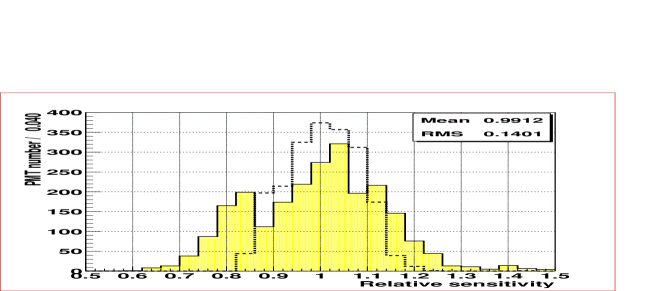
Figure 11: The relative sensitivity of the PMTs measured in the test facility (filled histogram) in comparison with the ETL provided measurements of the photocathode quantum efficiency at 420 nm.

2.6 Test procedure

Before the installation in the test facility the PMTs were labelled. 60 PMTs were tested in one cycle of operation. The PMTs were installed in the test facility in random positions on the test tables and with random orientations of the dynodes plane. No special measures were undertaken in order to prevent the illumination of the photocathodes before settling them on the test tables. After leaving the PMTs in the dark for a couple of hours, the nominal voltage provided by the manufacturer was applied to the PMTs and the dark rate checked. In the case of a PMT with a too high dark rate, the voltage has been decreased in order to ensure stable dark count rate at the level of less than 50 Kcps, and in addition the PMT was left under dark conditions for a longer period of time (up to one week).

At the beginning of the test the expected current was calculated using the known resistance of the high voltage divider and the operating high voltage. If the deviation from the calculated value did not fall in the fiducial interval, the PMT was examined more thoroughly. After these preparative stages, the high voltage adjustment started as described below (section 3). After the HV tuning finished, the PMTs dark rates and currents were checked once more. The PMTs still showing any kind of problem were excluded from the current test, left under lower HV and reexamined after a couple of days.

2.7 Software

A special data acquisition (DAQ) and analysis software have been developed for the test system. The kernel of the DAQ program was developed in 1992-1993 using Borland Turbo-C 3.0 under the MS-DOS operating system with a computer on the base of an Intel 486 processor. Following the rapid development of the computers, the program was adjusted to match more powerful processors, and in its present state the data acquisition speed is limited only by the hardware used. Now the program is running in the MS-DOS emulator under a Linux system.

The program provides control over all CAMAC settings of the electronics (delays, thresholds, signals width etc) and high voltage supplies. The program allows to specify the time period to save histograms on disk, the time period to check the pedestal positions, the time period to check PMT currents and high voltages, and the time period to check the dark rate. The period of data taking was defined either by setting the maximum number of events to be acquired, or by setting the run time. The program provides also the possibility of the automatic switching to the next group of PMTs, after the acquisition with the current group is finished.

The ADC pedestals are defined at the beginning of each specified period and, if a shift of the position is found, the appropriate correction is applied to the measured charges. In this way the low-frequency drift of the pedestal (mainly due to the small daily temperature variations) is compensated.

The PMT currents are checked every specified time period and, if the current is too high, the corresponding PMT is switched off automatically.

In the “pmt acceptance test” the data is acquired in the form of 3 histograms of 1024 bins each: the charge spectrum (ADC), the time of arrival of the response (TDC), and the afterpulse spectrum up to 32 $\mu s$ (MTDC). The mean acquisition rate is about 1000 events per second with 32 channels.

The DAQ program can be run in a “pmt gain tuning” mode. The operation in this mode is described in more detail in the following section.

In the “dst” mode of operation the data is written in a file after each event, allowing to study correlations in the data. This mode has been used in the optic fibers test [13].

The analysis software was developed on the base of the CERN ROOT libraries under a Linux system [22]. The program automatically analyses the charge spectrum, the transit time spectrum, and the spectrum of the ionic afterpulses and then plots all the data in the test sheet (see Fig.9 for an example). All numerical data is inserted in a database immediately.

3 Electron multiplier gain measurements and operating voltage setting

3.1 Brief description of the algorithm used

For the HV tuning it is necessary to provide a robust method of gain measurement. A method of photomultiplier calibration with high precision of up to a few percent has been discussed in [23]. The method is based on precision measurements of the PMT charge response to low intensity light pulses from a laser. It has been concluded that the precision of the method is limited only by the systematic errors in the discrimination of the small amplitude pulses from the electronics noise. On the basis of our experience with the precise PMT calibration [23], a fast procedure of PMT voltage tuning has been realized for the Borexino PMT test facility [24].

The goal of the tuning is to find the HV value that will provide an electron gain factor $k=2\cdot 10^{7}$ for each PMT. The mean value of the charge single electron response (SER), $\>q_{1}$, is determined, and the HV is adjusted so that $q_{1}$ agrees with a calibration value $c_{1}=1.6\>pC$ to a predefined precision. In [24] was shown that for small $\mu$ one can use the following approximation for $q_{1}$:

$$q_{1}=q_{m}\frac{1-\frac{\mu}{2}-p_{t}}{1-p_{t}\frac{thr}{2}},$$ (2)

where $q_{m}$ is the mean value of the cut distribution (a software cut of $15\%$ of $c_{1}$ is used in order to avoid the effects of the SER shape distortion near the hardware threshold);

$\mu$ is the mean p.e. number registered for one laser pulse;

$p_{t}$ is the part of the charge SER under the threshold. For the 15% software threshold, the value $p_{t}\cong 0.11$ was used, defined during the tests of the 100 PMTs for the CTF;

$thr$ is the threshold level measured in units of $c_{1}$(0.15 in the our case).

The mean p.e. number is defined during the test by estimating the probability of two sequential non-zero signals on PMT. Assuming a Poisson distribution of the light detection process, one can write:

$$\mu=-\ln(1-\frac{N_{ev}}{N_{Triggers}})\simeq\frac{N_{ev}}{N_{Triggers}},$$ (3)

where $N_{Trigger}$ is the the full number of the system triggers and $N_{ev}$ is the number of events that are followed by the non-zero pulse (the first signal in a two pulses sequence is triggering the system and thus is always present). In practice, we take as $N_{Trigger}$ the number of the events in the charge histogram (i.e. with a $5\%-10\%$ hardware cut), and as $N_{ev}$ we take the number of events after a 30 $\mu s$ delay estimated from the Multihit TDC histogram (see Fig.9). For these events the hardware cut on the CFD is about $20\%$ of the SER. The precision of the $\mu$ estimation using these $N_{Triggers}$ and $N_{ev}$ values is approximately $10\%$, which is good enough for our purpose.

The relative variation of the gain versus the variation of the applied voltage was defined in [24], performing the measurements of the gain changes with applied voltages for 4 different PMTs:

$$\frac{dk}{k}=(11-n)\cdot\frac{dU}{U-U_{D_{1}}},$$ (4)

with a constant factor $n\simeq 3.5$. $U_{D_{1}}=600$ V is the voltage difference between the first dynode and the photocathode, the stability of $U_{D_{1}}$ is provided by 3 Zener diodes of 200 V each (see Fig.1).

The HV correction in the automated system is calculated in the following way. If the deviation is bigger than $10\%$ the correction is set to a fraction of the maximum deviation of 100 V in proportion : $(\frac{q_{1}-c_{1}}{c_{1}})$ to the deviation from the calibration value. The value of 100 V is used, so that any possible over-voltage is avoided. For smaller deviations from the calibration the correction can be calculated more precisely from (4), namely:

$$\Delta U=-\frac{3}{2}\frac{U-U_{D_{1}}}{11}\frac{q_{1}-c_{1}}{c_{1}}.$$ (5)

3.2 Results of operating voltage tuning

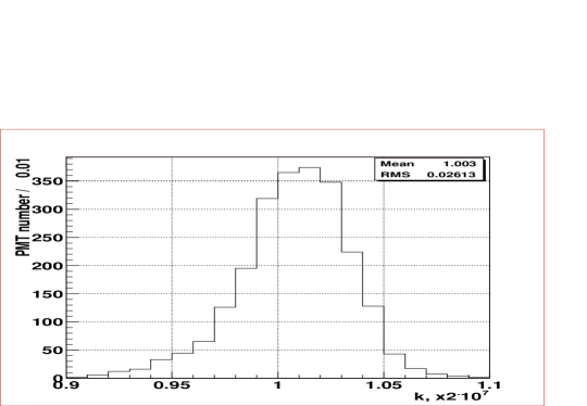
Figure 12: Results of the PMT gain tuning.

The algorithm is sufficiently fast; for 30 PMTs at 1 Kcps acquisition rate the HV is adjusted in 15-20 minutes with $2\%$ statistical precision.

The results of the HV tuning with the precision set to $2\%\>$ are presented in Fig.12. These results were obtained during the high precision tests after the HV adjustment. The mean value of k agrees with the expected $k=2.0\times 10^{7}$. Statistics for the operating voltage is shown in Fig.13.

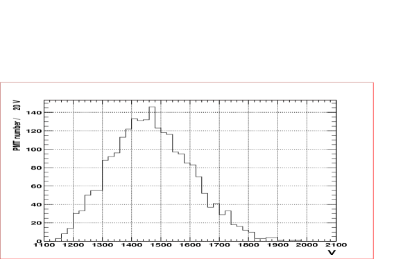
Figure 13: Operating high voltage for 2000 PMTs

The systematic error of the method is connected mainly with the substitution of the parameter $p_{t}$ by its mean value $p_{t}=0.11$, the error caused by the precision of $\mu$ estimation is negligible. The measured variance of the $p_{t}$ parameter is $\sigma_{p_{t}}=0.018$ [24]. As follows from the formula (2) the contribution of the systematic error is equal to $\sigma_{p_{t}}$. Summing quadratically the systematic (0.018) and the statistical (0.02) errors one will obtain the full error of $\sigma\simeq 0.027$. The variance of the gain distribution (0.028) agrees with the calculated value.

The method is not based on any specific single photoelectron spectrum model and hence can be used for the gain adjustment of the PMT with an arbitrary single electron response. Other advantages of the method are the simplicity of calculations, the predictable precision and very high speed of the algorithm. The method can be adapted for use with any type of PMT designed to operate in single electron regime.

4 Database

The PostgreSQL [25] database was prepared and filled with the data obtained during the tests. The data provided by the manufacturer (ETL) were put in another table of the same database, giving the possibility of easy access to the data. the complete description of all database entries is described in [26]. The main parameters put in the database are presented in Tables 4-6. These are mainly the parameters obtained directly in the test or after the processing of the data. For the description of the PMT charge spectrum the phenomenological model of the PMT charge spectrum was used as described in [23], an example of the fit is presented in Fig.9. Complete information on the measured parameters will be provided elsewhere [28].

Table 3: PMT data

	Brief description of the database field
HV	PMT Voltage corresponding approximately to the k=$2\times 10^{7}$electronic gain
k	Precise value of the PMT electron gain (in $2\cdot 10^{7}$units)
$f_{dark}$	Dark rate of the PMT in Kcps defined during the test. The threshold for
	the counter is the same as for the TDC (see tdcth)
$S$	Stability of the dark rate (variance of the observed dark rate divided by the
	square root of the dark rate, for the stable dark rate should be close to 1)
$rs$	Relative PMT sensitivity

Table 4: PMT Charge Spectrum data

	Brief description of the database field
$q_{1}$	Mean value of the SER charge spectrum (pedestal is subtracted)
	estimated from the data
p/v	Peak to Valley ratio
$\mu$	Mean value of photoelectrons per laser trigger defined from the
	Charge Spectrum Histogram as $\mu=-ln(\frac{N_{ped}}{N_{Trigger}})$
$rs$	Relative PMT sensitivity
	Relative variance of the Single Electron Response charge Spectrum
$v_{1}$	(i.e. $\frac{\sigma_{q_{1}}^{2}}{q_{1}^{2}}$, where $\sigma_{q_{1}}$and $q_{1}$are the rms and mean value of the SER
	charge Spectrum) estimated for the data
$p_{t}$	Part of the SER charge spectrum under the TDC (hardware) threshold tdcth
	(estimated without fit)

Table 5: The parameters of the model of single electron charge spectrum

	Brief description of the database field
$\mu$	Mean value of photoelectrons per laser trigger defined from the fit.
$q_{1}$	Histogram mean value of the SER charge Spectrum (estimated from the fit)
$v_{1}$	Relative variance of the Single Electron Response charge Spectrum
	calculated from fit values.
$q_{0}$	Mean of the Gaussian part of SER charge spectrum
$s_{0}$	RMS of the Gaussian part of SER charge spectrum
$p_{U}$	Fraction of the the events under the exponential part of SER (underamplified)
$A$	Slope of the exponential part of SER

Table 6: PMT transit time characteristics

parameter	Brief description of the database field
tdcth	Threshold of the CFD calculated from the events number in the TDC
	histogram (in p.e.)
$t_{0}$	position of the Gaussian peak on the TDC histogram ([ns])
$\sigma_{t}$	rms of the Gaussian peak on the TDC histogram ([ns])
$p_{late}$	late pulsing in percents (estimated as the ratio of the events in
	[t0+3tsig;100 ns] range to the events number under the Gaussian peak)
$p_{early}$	early pulses in percents (estimated as the ratio of the events in
	[0;t0-3tsig ns] range to the events number under the Gaussian peak)

Table 7: Afterpulses characteristics

parameter	Brief description of the database field
$a_{1}$	percentage of afterpulses in the [0.4-1.0] $\mu s$ range
$a_{2}$	percentage of afterpulses in the [1.0-3.6] $\mu s$ range
$a_{3}$	percentage of afterpulses in the [3.6-12.4] $\mu s$ range
$a_{tot}$	percentage of afterpulses in the [0.4-12.4] $\mu s$ range

5 Concluding remarks

The main task of the test system was the acceptance test of the Borexino PMTs. The system proved to be very efficient, 2350 PMTs delivered from the manufacturer were tested in 4 months of continuous system operation. The results of the test were analyzed and will be reported elsewhere [28]. Electronics and software of the test system have been used also in the Borexino Muon Veto PMTs test; in Borexino light fibers tests [13]; in testing of 120 PMTs for the upgrade of the CTF detector; in the charge spectrum study of the PMT [23]; in time characteristics high precision study of ETL9351 type PMT [27]; and in the study of the sensitivity of the PMT to the Earth magnetic field [21].

6 Acknowledgements

We are deeply grateful to G.Bacchiocchi, R.Cavaletti, R.Dossi, D.Giugni, P.Saggese, S.Grabar, and R.Scardaoni who were involved in various activities during the test facility installation, and in particular to G.Korga and L.Papp who took an active part in the test. We also thank the LNGS staff for the warm atmosphere and the good working conditions. The job of one of us (O.S.) was supported by the INFN sez. di Milano, and he is personally indebted to Prof. G.Bellini for the possibility to work at the LNGS laboratory. The authors appreciate the help of M.Laubenstein in preparation of the manuscript.

Credit is given to the developers of the CERN ROOT program [22], that was used in the calculations and to create all the figures of the article; as well as to the developers of the PostgreSQL database [25].

References

- [1] C. Arpesella et al “Borexino at Gran Sasso - Proposal for a real time detector for low energy solar neutrino.” Volume 1. Edited by G. Bellini, M. Campanella, D. Guigni. Dept. of Physics of the University of Milano. August 1991.
- [2] G. Alimonti et al., BOREXINO Collaboration, Astroparticle Physics 16 (2002) 205-234.
- [3] G. Ranucci, R. Cavaletti, P. Inzani, I. Manno, NIM A324 (1993) 580.
- [4] G. Ranucci et al, NIM A330 (1993) 276.
- [5] G. Ranucci et al, NIM A333 (1993) 553.
- [6] G. Ranucci et al, NIM A337(1993) 211.
- [7] Photomultipliers and Accessories, Electron Tubes Ltd., p.56.
- [8] C. Arpesella et al, Astroparticle Physics 18 (2002) 1-25.
- [9] C.R. Wuest et al., NIM A239 (1985) 467.
- [10] A. Baldini et al., NIM A372 (1996) 207.
- [11] C.J. Jillings at al., NIM A373 (1996) 421.
- [12] G. Alimonti et al, NIM A 406 (1998) p.411-426.
- [13] B. Caccianiga et al, NIM A496 (2003) 353-361.
- [14] G. Bacchiocchi et al, LNGS preprint INFN/TC-97/35, 1997. Available at http://lngs.infn.it/.
- [15] K. Caputa and M.A. Stuchly IEEE Transaction and Measurements, vol. 45, No. 3, (1996).
- [16] S.M. Rubens Rev. Sci. Instrum. 16(9), (1945).
- [17] R. Merritt et al. Rev. Sci. Instrum. 54(7), (1983).
- [18] R. Grisenti and A. Zecca Rev. Sci. Instrum. 52(7), (1981).
- [19] R.K. Cacak and J.R. Craig, Rev. Sci. Instrum., 40, 1468 (1969).
- [20] M. Ference et al., Rev.Sci.Instrum. 11,57(1940).
- [21] A. Ianni, G. Korga, G. Ranucci, O. Smirnov, A. Sotnikov, LNGS preprint INFN/TC-00/05, 2000.
- [22] ROOT home page, http://root.cern.ch/.
- [23] R. Dossi, A. Ianni, G. Ranucci, O. Ju. Smirnov, NIM A451 (2000) 623-637.
- [24] O. Ju. Smirnov. Instruments and Experimental Techniques, Vol.45 No3 (2002) 363.
- [25] PostgreSQL home page http://www.postgresql.org/.
- [26] O. Ju. Smirnov. CTF-II Photomultipliers database. BOREXINO PMT working group home page at http://www.pcbx01.lngs.infn.it
- [27] O.Ju. Smirnov, P. Lombardi, and G. Ranucci, Instruments and Experimental Techniques, Vol.47 No 1 (2004) p.69-77; also in arXiv:physics/0403029.
- [28] A. Ianni, P. Lombardi, G. Ranucci and O. Smirnov. “The measurements of 2200 ETL9351 type photomultipliers for the Borexino experiment with the photomultiplier testing facility at LNGS”, arXiv:physics/0406138, submitted to NIM.