Reconstruction of spatially inhomogeneous dielectric tensors via optical tomography
Abstract
A method to reconstruct weakly anisotropic inhomogeneous dielectric tensors inside a transparent medium is proposed. The mathematical theory of Integral Geometry is cast into a workable framework which allows the full determination of dielectric tensor fields by scalar Radon inversions of the polarization transformation data obtained from six planar tomographic scanning cycles. Furthermore, a careful derivation of the usual equations of integrated photoelasticity in terms of heuristic length scales of the material inhomogeneity and anisotropy is provided, making the paper a self-contained account about the reconstruction of arbitrary three-dimensional, weakly anisotropic dielectric tensor fields.
OCIS numbers 100.3190, 160.1190, 080.2710
I Introduction
The inverse boundary value problem of recovery of anisotropic spatially varying electromagnetic properties of a medium from external measurements at a fixed frequency is among the most mathematically challenging of inverse problems. For low-frequency electromagnetic measurements where a static approximation is valid, an anisotropic dielectric tensor or conductivity tensor is uniquely determined by complete surface electrical measurements up to a gauge conditionLassas and Uhlmann (2001). For isotropicOla, Päivärinta and Somersalo (1993) and chiral isotropic mediaJoshi and McDowall (2000) a knowledge of all pairs of tangential electric and magnetic fields at the boundary, for a single non-exceptional frequency, is known to be sufficient to recover the material properties. Anisotropic materials are important in many practical problems with anisotropy arising from, for example, flow, deformation, crystal or liquid crystal structure, and effective anisotropic properties arising from homogenization of fibrous or layered composite materials. For general anisotropic media the question of sufficiency of data for reconstruction remains open.
In this paper we concentrate on a specific high-frequency case of considerable practical importance. We assume that the material is non-magnetic, i.e. has a homogeneous and isotropic permeability equal to the vacuum value ; that the conductivity is negligible; and that the permittivity, or dielectric tensor, is weakly anisotropic in a sense that will be defined below. We present a mathematical framework which allows us to invert the polarization transformation data obtained from tomographic measurements of light rays passing through an optically anisotropic material at sufficiently many angles for the six independent components of the (spatially varying) dielectric tensor inside the specimen. It will be shown that, for weak anisotropy, our method allows the full determination of all tensor components, provided that tomographic measurements are made for six carefully chosen orientations of the planes in which the light rays scan the medium.
The equations describing the passage of light through inhomogeneous and weakly anisotropic media have been formulated in Refs. Kravtsov, 1968; Kravtsov and Orlov, 1980; Fuki et al., 1998, and in section II we shall show how to obtain these equations from a geometric-optical starting point by expanding the electric field in powers of appropriate length scales which describe the inhomogeneity and anisotropy of the medium. Also, a condition for “weak” anisotropy will be specified upon which we shall linearize (section IV) the equations determining the polarization transfer matrix along the light rays. In section V we then present our method of reconstructing the permittivity tensor in the linearized limit by performing scalar Radon transforms on the polarization transformation data obtained from six scanning cycles on different planes intersecting the specimen. In section VI the method is demonstrated by giving a visual example of reconstruction of the permittivity tensor inside an axially loaded cylindrical bar: in this case, the stress tensor in the (transparent) medium gives rise to optical anisotropy, and it will be seen that our method works well in the limit of weak anisotropy. The mathematical basis for this method has been anticipated in the seminal work of SharafutdinovSharafutdinov (1994), whose book contains a general theory of “ray transforms” of tensor fields on -dimensional Euclidean spaces, and an examination into the possibility to invert them for reconstructing the underlying tensor fields. Our work presented here is an adaption, and partial reformulation, of this highly mathematical framework, to the specific objective of reconstructing inhomogeneous dielectric tensor fields via optical tomography.
It should be mentioned that the determination of anisotropic dielectric tensors as presented here has a closely related variant in the problem of reconstruction of a stress tensor field inside a loaded transparent material; the phenomenon that an initially isotropic medium becomes optically anisotropic when under strain is called Photoelasticity Frocht (1948); Coker and Filon (1957); Theocaris and Gdoutos (1979); Jessop and Harris (1949); Hendry (1966) and may be used to obtain information about the internal stress in a strained medium from polarization transformation data obtained by tomographical methods. The photoelastic effect as a means to retrieve information about internal stresses has been studied extensively: A method termed “Integrated Photoelasticity”Aben (1966, 1979); Aben et al. (1989); Aben and Guillemet (1993); Aben and Puro (1997) is well-known, and it was pointed outDavin (1969); Aben et al. (1990, 1991, 2003) that information about the difference of principal stress components could be retrieved from appropriate Radon transformations of polarization transformation data. However, these methods do not succeed in reconstructing the stress components separately and therefore the full stress tensor, and the linearly related dielectric tensor, can be obtained in this way only for systems exhibiting a certain degree of symmetry, such as an axial symmetry. Other methods of reconstruction have been suggested, for example, a three-beam measurement schemeAndrienko and Dubovikov (1994), where for axisymmetric systems an onion-peeling reconstruction algorithm was proposedAndrienko et al. (1992a, b). Another method, which in principle is capable of determining a general three-dimensional permittivity tensor, is the “load incremental approach”Wijerathne et al. (2002). Here, the stress on the object is increased in small increments, and at each step, a measurement cycle is performed.
The new results in this paper are twofold: Firstly, we derive the set of equations determining the polarization transfer matrices for a given light ray scanning the object. These equations are somewhat related to the standard equations of integrated photoelasticityAben (1979), but here we present a more rigorous exposition of the heuristic length scalesFuki et al. (1998), and the approximations based thereupon, which underlie the usual derivation of these equations from Maxwell’s equations in a material medium; this is done in sections II, III and IV. Secondly, we present a novel scheme for reconstruction of arbitrarily inhomogeneous dielectric tensors in the interior of the specimen, subject only to the condition that the birefringence is “weak” in a sense which will be specified in sections V and VI.
II Heuristic length scales
It is assumed that the material is non-absorbing for optical wavelengths, and furthermore is non-magnetic, , where is the magnetic permeability of vacuum. As for the permittivity we assume that the dielectric tensor deviates “weakly” from a global spatial average
| (1) |
where denotes the body having a volume , is the trace operation, and is the dielectric tensor. In a zero-order approximation the material therefore may be regarded as homogeneously isotropic, with scalar dielectric constant as defined in (1). Typically, this behaviour of weak deviation from a homogeneously isotropic background will be satisfied for glasses and certain resins under moderate internal stress or external load. The scalar constant of permittivity will be a reference quantity when we specify the dimensionless degree of anisotropy in eq. (8).
For the actual problems relevant to our work, the length scales characterising inhomogeneities in the material are much larger than the wavelength of the (monochromatic) light passing through the object, so that the usage of geometric-optical approximations is justified. Heuristically, two such length scales can be conceptualizedFuki et al. (1998): A scale characterising the degree of inhomogeneity may be introduced by
| (2) |
where denotes a unit vector in the direction of wave propagation. Furthermore, in any anisotropic medium, two preferred polarization directions , , for each given direction of wave propagationBorn and Wolf (1999); Fowles (1975); Sommerfeld (1954); Ditchburn (1976); Longhurst (1973), exist at each point, so that a scale measuring the rate of variation in these polarization directions can be speficied by
| (3) |
These scales should be compared to the average wavelength of the monochromatic light passing through the medium, so that, when the limit
| (4) |
is satisfied, the (complex) electric field may be given in the form
| (5) |
where the eikonal describes a locally-plane wave with wave vector , and the amplitude varies weakly on the length scale . Motivated by these considerations, Fuki, Kravtsov, Naida (FKN)Fuki et al. (1998) introduce a dimensionless scale
| (6) |
The limit of geometrical optics then can be specified by the condition
| (7) |
We also need an explicit measure of anisotropy
| (8a) | ||||
| (8b) | ||||
where is an appropriate number characterising the magnitude of the components of the dimensionless anisotropy tensor , such as a global maximum, etc. If anisotropy is not weak, then at each point in the medium we have a continuous splitting of rays due to the fact that there are two distinct phase velocities, and two distinct ray velocities, for any given propagation direction. A condition for weak anisotropy therefore arises if we demand that the passage of light through the material can be described by a single ray which is influenced by the local variations of the optical tensors only in the way that the polarization directions rotate. This is the situation that commonly occurs in photoelasticity and is also of greatest interest to our work.
It was shown by FKNFuki et al. (1998) that ray splitting can be ignored, if
| (9) |
In this caseFuki et al. (1998) “it is impossible to discriminate experimentally between split rays”, and one can effectively replace the two rays by a single isotropic ray which is obtained from the isotropic part of the dielectric tensor alone. This is indeed the domain we are most concerned with, since experimentally no ray splitting is seen in photoelastic experiments. In fact, for those applications we are interested in it is usually true that light propagates along straight lines through the specimen, so that the trial solution (5) may be replaced by an even stronger ansatz
| (10) |
with constant wave vector , just as for a plane wave. The phase velocity associated with this wave vector is the one associated with the average permittivity defined in eq. (1),
| (11) |
However, the amplitude has a spatial dependence which accounts for the variation of the two preferred polarization directions along the light ray.
Under the conditions (7) and (9), the electric field and electric displacement behave like
| (12) |
This means that is nearly transverse, while the same is true for only if we assume in addition that the degree of anisotropy is small,
| (13) |
This is the condition of weak anisotropy, and our method is formulated for this “quasi-isotropic” regime.
III Equations satisfied by the transfer matrices
The information about the change in the state of polarization of a light beam passing through the material is encoded in a two-dimensional unitary transfer matrix. The equation satisfied by the transfer matrix along a light ray is given in most accounts on photoelastic tomographyDavin (1969); Aben et al. (1990, 1991, 2003); Andrienko and Dubovikov (1994); Andrienko et al. (1992a, b), but the various approximations taken in the process of neglecting higher powers of ratios and are not always stated clearly; we therefore briefly summarize the necessary steps here:
On inserting (10) into Maxwell’s equations we obtain
| (14) |
It is easy to show that
| (15) |
hence the term can be neglected in the geometrical-optical limit (7). Then (14) takes the form
| (16) |
where was given in eq. (11). The longitudinal component of eq. (16), obtained by projection onto the unit vector in the direction of propagation of the light beam, is of the order
| (17) |
and is neglected in the geometrical-optical limit. Hence we only retain the transverse components of and , i.e. the components perpendicular to the wave propagation .
Now let us study eq. (16) in a coordinate system in which the direction of propagation is along the axis. Then (16) becomes
| (18) |
where was defined in eq. (8a). The solution of (18) can be expressed via a transfer matrix
| (19) |
where satisfies an ordinary differential equation similar to (18), together with initial condition
| (20) | ||||
Eqs. (20) can be expressed as an integral equation
| (21) |
where denotes the matrix of transverse components of as they appear in eq. (18). A formal solution of (21) is given by the Born-Neumann series
| (22) |
The transfer matrix is unitary and thus preserves the norm of the complex electric field vector. Physically this means that intensity is preserved, so unitarity here just expresses energy conservation of the light ray. This must indeed be the case, since we have assumed a non-absorbing medium.
IV The linearized inverse problem
Assuming that the transfer matrices have been determined for sufficiently many light rays scanning the medium, the associated inverse problem now consists in reconstructing the anisotropy tensor from the collection of these transfer matrices; this inverse problem is obviously non-linear in , as can be seen from eqs. (21 and 22). The solution to the fully non-linear problem is not known as yet. However, in the quasi-isotropic regime we can deal with the linearized inverse problem: this is defined by a truncation of the Born-Neumann series in (22) after the first-order term
| (23) |
For example, for a relative anisotropy of , a wavelength of m and assuming a length of m of the object, we find that the first-order term in (23) is of the order , hence the linearization will be a good approximation in this case.
The transfer matrices must be determined by suitable measurements of the change of polarization along each light ray passing through the medium at many different angles, possibly including interferometric methods. By measuring three so-called characteristic parametersAben (1966) the -factor of the transfer matrices can be computed using the Poincaré equivalence theoremPoincaré (1892), a matrix decomposition theorem which allows to interprete the characteristic parameters as the retardation angle , the angle of the fast axis , and the rotation angle of an equivalent optical model consisting of a linear retarder and a rotator with these optical parameters. The Poincaré equivalence theorem can be formulated in terms of Jones matrices or Stokes parameters on the Poincaré sphere; a contemporary exposition of these relations was given recently in Ref. Hammer, 2004.
Thus, the measurement of determines a unimodular matrix such that
| (24) |
where is the global phase of the transfer matrix . In the general case, assuming no restrictions on the degree of anisotropy, this global phase can be arbitrarily large, and furthermore cannot be determined from the characteristic parameters alone, but must be measured e.g. through interferometric methods, for each given light ray. However, in the limit of weak anisotropy, the global phase is effectively determined by the characteristic parameters alone: Suppose that the unimodular matrix has been computed by measuring the parameters using the Poincaré equivalence theorem; from eq. (23) it then follows that the unknown phase must be chosen so as to make the real parts of the diagonal (non-diagonal) matrix elements equal to one (zero),
| (25) | ||||
We can therefore determine the phase from any of these equations, or, for the sake of numerical stability, from all of them, so as to obtain an average value of . Thus, in the weak-anisotropy limit, the number of real “degrees of freedom” in the transfer matrices is effectively equal to three, rather than four as in the general case.
V Solution of the linearized inverse problem by six scalar Radon inversions
We now show that the linearized inverse problem can be reduced to six scalar Radon inversions performed on the polarization transformation data. We first specify a plane in which intersects the specimen and contains the point ; the orientation of the plane is determined by a unit vector normal to the plane. Consider the straight line with unit vector lying in , describing a light ray passing through the specimen and lying in the given plane . Let be a third unit vector, orthogonal to and in such a way that form a right-handed system. Then the equation describing the polarization transformation along the light ray in the direction is given by the analogue of (23),
| (26) |
The measurement of characteristic parameters determines the transfer matrix on the left-hand side of (26). We now repeat these measurements for all lines lying in the given plane and thus obtain a collection of line integrals for the normal component in ,
| (27) |
for any pair of directions and ; we could extend the limits of integration in (27) to , since in practical situations the object will be placed inside a tank with a phase-matching fluid, hence the value of outside the object is zero. The set of line integrals in (27), taken for all light rays in , is called the transverse ray transformSharafutdinov (1994) of with respect to .
However, the component is perpendicular to the plane and is therefore invariant under rotations in that plane, so that it behaves like any other scalar function defined on . It follows that the collection of integrals (27) is indeed the standard 2D Radon transformHelgason (1980) of the scalar function , , and hence can be inverted for the component using any numerical scheme for Radon inversion appropriate to the circumstances, such as filtered back-projectionNatterer (1986). This produces the component for every point in the plane .
On repeating the same process for all planes parallel to we reconstruct the component within the whole specimen.
We now perform this procedure for the following six different choices of the vector :
| (28a) | |||
| (28b) | |||
The scan-and-reconstruction cycle for the choices in (28a) produces components
| (29) |
of the anisotropy tensor. On the other hand, for the choices in (28b) we obtain the following result: Let us focus attention on the first orientation , where the associated reconstruction gives us the tensor component everywhere within the object. But, due to the fact that the tensor is linear in its arguments, this component can be expressed in the form
| (30) |
where we have used the fact that is symmetric and hence . Thus, having already reconstructed and everywhere in the specimen, we can immediately compute from the reconstructed values of using eq. (30). On repeating this process for the last two choices of in (28b) we see that all six tensor components of can be reconstructed in this way.
If the average dielectric constant of the object is known we can compute the full dielectric tensor immediately using the definition (8a). On the other hand, if is not determined we can still use (8a) to write
| (31) |
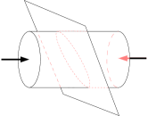
in other words, we can reconstruct up to a scale factor ; this may still produce valuable information about the internal structure of the dielectric material, see Fig. 1.
VI Numerical example
Here we present a numerical example of reconstruction of a single tensor component for a plane intersecting the object at an oblique angle. The polarization transformation data are obtained from an artificial stress model of a cylindrical bar with a circular cross-section which is subject to axial load and in turn bulges out in the middle section, see Fig. 1(a).
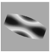
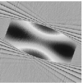
Based on these artificial forward data we then employ our method and reconstruct the “normal” component on a plane passing through the center of the cylinder and making an angle of with the symmetry axis, see Fig. 1(b). The original plot of in this plane is shown in Fig. 1(c); the reconstructed image in Fig. 1(d) has pixels, assuming that scans, one scan on every , have been performed in the plane. It will be seen that the reconstruction contains artefacts which are typical of a Radon inversion; they can be reduced by increasing the number of scans, e.g., by performing one scan on each degree, for a total of scans. The result in this case is almost indistinguishable from the original in Fig. 1(c) so that we have refrained from showing it.
For the inverse Radon transformation, the Matlab function iradon has been used which utilizes a filtered back-projection algorithmNatterer (1986).
VII Summary
We have presented a novel way to reconstruct an arbitrarily inhomogeneous anisotropic dielectric tensor inside a transparent non-absorbing medium, under the conditions that the birefringence is a deviation from a homogeneous isotropic average, and that this deviation is weak. It was shown that the associated linearized inverse problem of reconstructing the dielectric tensor from polarization transformation data gathered by optical-tomographical means can be reduced to six scalar Radon inversions which allow the determination of the permittivity tensor completely. We also supplied a more rigorous derivation of the usual equations of integrated photoelasticity which define the inverse problem for the dielectric tensor; our exposition was based on a careful description of the various approximations that enter the derivation of the photoelasticity equations from Maxwell’s equations in a material medium.
Acknowledgements
The authors acknowledge support from EPSRC grant GR/86300/01.

References
- Lassas and Uhlmann (2001) M. Lassas and G. Uhlmann, Ann. Sci. École Norm. Sup.(4) 34, 771 (2001).
- Ola, Päivärinta and Somersalo (1993) P. Ola and L. Päivärinta, E. Somersalo, Duke Math. J. 70, 617 (1993).
- Joshi and McDowall (2000) M. Joshi and S. McDowall, Pacific J. Math 193, 107 (2000)
- Kravtsov (1968) Y. A. Kravtsov, Dokl. Akad. Nauk. SSSR 183, 74 (1968).
- Kravtsov and Orlov (1980) Y. A. Kravtsov and Y. I. Orlov, Geometric Optics of Inhomogeneous Media (Nauka, Moscow, 1980).
- Fuki et al. (1998) A. A. Fuki, Y. A. Kravtsov, and O. N. Naida, Geometrical Optics of Weakly Anisotropic Media (Gordon and Breach Science Publishers, Amsterdam, 1998).
- Sharafutdinov (1994) V. A. Sharafutdinov, Integral Geometry of Tensor Fields (VSP, Netherlands, 1994).
- Frocht (1948) M. M. Frocht, Photoelasticity, vol. 1+2 (John Wiley, New York, 1948).
- Coker and Filon (1957) E. G. Coker and L. N. G. Filon, Photo-Elasticity (Cambridge University Press, Cambridge, 1957), 2nd ed.
- Theocaris and Gdoutos (1979) P. S. Theocaris and E. E. Gdoutos, Matrix Theory of Photoelasticity, Springer Series in Optical Sciences (Springer Verlag, Berlin, 1979).
- Jessop and Harris (1949) H. T. Jessop and F. C. Harris, Photoelasticity (Cleaver-Hume, London, 1949).
- Hendry (1966) A. W. Hendry, Photoelastic Analysis (Pergamon Press, Oxford, 1966).
- Aben (1966) H. K. Aben, Experimental Mechanics 6, 13 (1966).
- Aben (1979) H. Aben, Integrated Photoelasticity (McGraw-Hill, New York, 1979).
- Aben et al. (1989) H. K. Aben, J. I. Josepson, and K.-J. E. Kell, Optics and Lasers in Engineering 11, 145 (1989).
- Aben and Guillemet (1993) H. Aben and C. Guillemet, Photoelasticity of Glass (Springer-Verlag, Berlin, 1993).
- Aben and Puro (1997) H. Aben and A. Puro, Inverse Problems 13, 215 (1997).
- Davin (1969) M. Davin, C. r. Acad. Sci. A 269, 1227 (1969).
- Aben et al. (1990) H. Aben, S. Idnurm, and A. Puro, in Proc. 9th Internat. Confer. On Exp. Mech. (Copenhagen, 1990), vol. 2, pp. 867–875.
- Aben et al. (1991) H. Aben, S. Idnurm, J. Josepson, K.-J. Kell, and A. Puro, in Analytical Methods for Optical Tomography, edited by G. G. Levin (1991), vol. 1843 of Proc. SPIE, p. 220.
- Aben et al. (2003) H. Aben, A. Errapart, L. Ainola, and J. Anton, in Proc. Internat. Confer. On Advanced Technology in Exp. Mech (Nagoya, 2003), ATEM’ 03.
- Andrienko and Dubovikov (1994) Y. A. Andrienko and M. S. Dubovikov, J. Opt. Soc. Am. A 11, 1628 (1994).
- Andrienko et al. (1992a) Y. A. Andrienko, M. S. Dubovikov, and A. D. Gladun, J. Opt. Soc. Am. A 9, 1761 (1992a).
- Andrienko et al. (1992b) Y. A. Andrienko, M. S. Dubovikov, and A. D. Gladun, J. Opt. Soc. Am. A 9, 1765 (1992b).
- Wijerathne et al. (2002) M. L. L. Wijerathne, K. Oguni, and M. Hori, Mechanics of Materials 34, 533 (2002).
- Born and Wolf (1999) M. Born and E. Wolf, Principles of Optics (Cambridge University Press, Cambridge, 1999), 7th ed.
- Fowles (1975) G. R. Fowles, Introduction to Modern Optics (Holt, Winehart and Winston, Inc., New York, 1975), 2nd ed.
- Sommerfeld (1954) A. Sommerfeld, Optics, Lectures on Theoretical Physics, vol. 4 (Academic Press, New York, 1954), 1st ed.
- Ditchburn (1976) R. W. Ditchburn, Light (Academic Press, London, 1976), 3rd ed.
- Longhurst (1973) R. S. Longhurst, Geometrical and Physical Optics (Longman, London, 1973), 3rd ed.
- Poincaré (1892) H. Poincaré, Théorie mathématique de la lumiére (Carré Naud, Paris, 1892).
- Hammer (2004) H. Hammer, J. Mod. Opt. 51, 597 (2004).
- Helgason (1980) S. Helgason, The Radon Transform (Birkhäuser, Basel, Stuttgart, 1980).
- Natterer (1986) F. Natterer, The Mathematics of Computerized Tomography (Wiley, Teubner, Stuttgart, 1986).