A Simple Denoising Technique

The measurements of very low level signals at low frequency is a very difficult problem, because environmental noise increases in this frequency domain and it is very difficult to filter it efficiently. In order to counteract these major problems, we propose a simple and generic denoising technique, which mixes several features of traditional feedback techniques and those of noise estimators. As an example of application, large band measurements of the thermal fluctuations of a mechanical oscillator are presented. These measurements show that the proposed denoising technique is easy to implement and gives good results.

1 Introduction

The measurements of very low level signals at very low frequency (VLF) is a very difficult problem, because environmental and electric / magnetic noises often increase in this frequency domain. Furthermore, it is well known that the difficulties of isolating an experimental setup from these unwanted noise sources increase by reducing the measuring frequency. Typical examples are the screening of low frequency magnetic fields or the isolation of a measurement from the unwanted environmental vibrations. Many techniques have been proposed and accurately applied to reduce the effects of the unwanted noise sources.

The simplest techniques are of course the passive ones. Let us consider in some details the problem of vibration isolation (the magnetic field screening presents similar problems).

In a typical laboratory environment, vibrations transmitted through the floor normally have a frequency spectrum from dc to a few hundred Hz. The reduction of these vibrations is usually obtained by installing the experiment on floating tables which have horizontal and vertical resonance frequencies around 1 Hz. Thus, noise reduction is obtained only for frequencies larger than the natural resonant frequencies of the table. This is, of course, an excellent method for high frequency measurements, but at frequencies close to and smaller than 1 Hz this method becomes useless. Exactly at resonance, noise is even enhanced. To overcome these problems that appear at VLF, feedback techniques have been used. These techniques require detectors which measure the noise signals and actuators which reduce the acceleration of the table plate. Similar techniques are of course used for screening VLF magnetic fields. Indeed, high frequency magnetic fields are screened by Faraday cages and the VLF components are subtracted by a feedback technique [1].

Feedback techniques are widely used, but they are limited by the noise of the detectors and of the actuators. Their calibration is often very complex and requires very tedious operations in order to work properly. Furthermore, they can be only applied in all of the cases where the environmental noise can be accurately measured. When this is not possible and / or one is not interested in stabilizing a system on a given working point, but only in reducing the noise on a given signal, other techniques may be used. From the signal analysis point of view, most of the techniques that have been proposed and accurately applied to reduce the effects of the unwanted noise sources rely upon the knowledge of the response function of the system under study, and a guess about the noise, which is often supposed to be a random variable belonging to some class of signals, e.g. ergodic and second order stationary signals [2, 3, 4, 5, 6]. However, this guess is often limited.

The simple denoising technique proposed in this paper actually combines several aspects of the two above mentioned techniques. Indeed, in many cases one has access to the environmental noise, but one does not need to stabilize a setup on a given working point, but only to reduce the effect of the noise on a given signal. Therefore, rather than carrying out a somewhat sophisticated and expensive feedback system, which could even fail to solve the noise problem at VLF, we developped a simple denoising technique whose principle precisely lies in measuring the residual noise when passive “screening” devices are already used. The general principles and the limits of the new technique are described in Sec. 2.

This denoising technique was motivated by the study of the violation of the fluctuation dissipation theorem (FDT) in out of equilibrium systems as aging glasses. This is a subject of current interest which begins to be widely studied in many different systems [7, 8, 9, 10, 11]. Therefore, in Sec. 3 we propose an application of this new technique to the measurement of VLF mechanical thermal fluctuations. The experimental results, presented in Sec. 4, show the quality of the noise reduction. Finally, in Sec. 5 we discuss some other possible applications and we conclude.

2 A simple denoising technique

Suppose one has to measure a signal on which an external noise is superimposed. Let us call this signal the true signal $x_{\mathrm{true}}(t)$ and the external noise $x_{\mathrm{env}}(t)$, so that the measured signal can be written in the additive manner

$$x(t)=x_{\mathrm{true}}(t)+x_{\mathrm{env}}(t).$$ (1)

The only assumptions needed are that $x_{\mathrm{true}}(t)$ and $x_{\mathrm{env}}(t)$ are uncorrelated and both stationary processes (as we will see, the hypothesis of stationarity can be weakened), and can be written in an additive manner like in Eq. 1. In addition, we assume that one can directly measure $x$, whereas $x_{\mathrm{env}}$ is measured with a detector whose output signal is $x_{\mathrm{det}}(t)$. If the noise is small, in the limit of linear response theory, it can be stated that $x_{\mathrm{det}}$ is linearly related to $x_{\mathrm{env}}$, which means that there exists a hypothetical response function $\hat{R}_{\mathrm{d}}^{-1}(\omega)$ such that

$$\hat{x}_{\mathrm{det}}(\omega)=\hat{R}_{\mathrm{d}}^{-1}(\omega)\hat{x}_{\mathrm{env}}(\omega),$$ (2)

where $\hat{f}(\omega)=\int_{\mathbb{R}}f(t)e^{-i\omega t}dt$ is the Fourier transform of $f(t)$. Notice that no hypothesis is done on $\hat{R}_{\mathrm{d}}$, which is in principle unknown.

The Fourier transform of the true signal thus reads

$$\hat{x}_{\mathrm{true}}=\hat{x}-\hat{R}_{\mathrm{d}}\,\hat{x}_{\mathrm{det}}.$$ (3)

Assuming that the true and external noise signals are uncorrelated, that is $\langle x_{\mathrm{true}}\,x_{\mathrm{det}}^{*}\rangle=0$, one can compute the kernel $\hat{R}_{\mathrm{d}}$ as

$$\hat{R}_{\mathrm{d}}=\frac{\langle\hat{x}\,\hat{x}_{\mathrm{det}}^{*}\rangle}{\langle{|\hat{x}_{\mathrm{det}}|}^{2}\rangle},$$ (4)

where $\langle\cdot\rangle$ stands for the ensemble average. Thus Eqs. 3 and 4 allow us to compute the signal and its spectrum:

$$x_{\mathrm{true}}(t)=x(t)-\int_{\mathbb{R}}\hat{R}_{\mathrm{d}}(\omega)\hat{x}_{\mathrm{det}}(\omega)e^{i\omega t}\,\frac{d\omega}{2\pi},$$ (5)

and

$$\langle{|\hat{x}_{\mathrm{true}}|}^{2}\rangle=\langle{|\hat{x}|}^{2}\rangle-{|\hat{R}_{\mathrm{d}}|}^{2}\langle{|\hat{x}_{\mathrm{det}}|}^{2}\rangle.$$ (6)

Therefore, $x_{\mathrm{true}}$ can be computed from the simultaneous measurements of $x$ and $x_{\mathrm{env}}$.

We see that the hypothesis of stationarity is not really necessary, because $\hat{x}$, $\hat{R}_{{d}}^{-1}$ and $\hat{x}_{{det}}$ can be slowly varying functions of time, with a characteristic time $\tau$. In such a case, if the ensemble average is performed in a time ${T}$ such that ${T}\ll\tau$, then Eqs. 3, 4, 5 and 6 can be still applied on intervals of length ${T}$. This observation makes this simple technique very powerful, because the response of the system to the environmental noise can change as a function of time and of the external noise source. Thus, $\hat{R}_{\mathrm{d}}$ is a dynamical variable which can be computed in each time interval of length ${T}$, and which allows to retrieve the true signal.

However, the signal $x_{\mathrm{rec}}$ reconstructed using Eqs. 3, 4, and 5 will differ from $x_{\mathrm{true}}$ because of experimental errors. One source of error is the noise of the detectors and of the amplifiers, which introduces an extra additive noise term $\eta(t)$ in Eq. 1, which is uncorrelated with $x_{\mathrm{true}}$ and $x_{\mathrm{det}}$, thus $x_{\mathrm{rec}}(t)=x_{\mathrm{true}}(t)+\eta(t)$. However, $\eta$ can be done very small and it does not constitute the main source of error. The main one is the limited number $N$ of ensemble averages that can be done in the time ${T}$. This is very important because if $\hat{R}_{\mathrm{d}}$ is a slowly varying function of $t$, then one has to impose ${T}\ll\tau$ in order to retrieve the true signal. Finally, it has to be pointed out that the advantage of the technique is when the amplitudes of $x_{\mathrm{true}}$ and ${x}_{\mathrm{det}}$ are comparable, that is, when the signal to environmental noise ratio is either smaller than or equal to one.

The accuracy of the technique has been checked on several artificial signals. We have chosen for $x_{\mathrm{true}}$ and ${x}_{\mathrm{det}}$ either random or periodic signals. The random signals may be either colored or white noise with Gaussian or uniform distribution. To estimate the error of the reconstruction, we first consider the difference $\Delta$ between the reconstructed $x_{\mathrm{rec}}$ and $x_{\mathrm{true}}$, that is $\Delta(t)=x_{\mathrm{rec}}(t)-x_{\mathrm{true}}(t)$. We then compute the ratio $R_{\mathrm{rec}}$ between the rms of $\Delta$ and that of $x_{\mathrm{true}}$, which is a good indicator of the error of the reconstructed signal. As expected we find that $R_{\mathrm{rec}}\sim 1/\sqrt{N}$ for large $N$.

An example of the reconstruction is given in Fig. 1. We see that although the signal is completely erased by the noise (cf Fig. 1b) the reconstruction is quite good. It is obvious that this is an extremely simple example, but as we will see the technique becomes very interesting when $\hat{R}_{\mathrm{d}}$ is a slowly varying function of $t$.

To conclude this section, it should be stressed that, from the signal analysis point of view, we derived a method in a way similar to the Wiener filtering, which aim at separating (in an optimal sense, see [2, 3, 12]) two random signals $x_{\mathrm{true}}$ an $x_{\mathrm{det}}$, which are supposed to be ergodic second order stationary and uncorrelated random signals, and can be written in an additive manner like in Eq. 1. Then, we extended this denoising technique to nonstationary signals in a simple and original manner. In a more general study, nonstationary signals could be addressed to the Kalman filtering (also referred as to the Kalman-Bucy filtering), which can be considered as the extension of the Wiener filtering to the case of nonstationary signals [4, 5, 6].

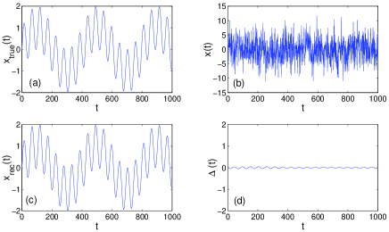
Figure 1: Artificial signal. (a) True signal as a function of time. In this example $x_{\mathrm{true}}(t)=\sin{\frac{2\pi}{51}t}\,+\sin{\frac{2\pi}{400}t}$. (b) The signal $x$ as a function of time. The noise is a Gaussian white noise of variance 4. (c) The reconstructed signal as a function of time. (d) Residual error $\Delta$ of the reconstruction as a function of time.

3 Application to thermal fluctuations measurements

In this section, we describe a useful application of this technique to the measurement of thermal fluctuations of a mechanical oscillator, whose damping is given by the viscoelasticity of an aging polymer glass. This is an important experimental measurement which is extremely useful in the study of the violation of the FDT in out of equilibrium systems, specifically in aging glasses. This violation is a subject of current interest which has been studied mainly theoretically [13, 14]. However, there are not clear experimental tests of these theoretical predictions, which have to be checked on real systems by studying the VLF spectra of mechanical thermal fluctuations. Thus, the main purpose of our study is to have a reliable measurement of this VLF spectra in an aging polymer.

To study this spectrum, we have chosen to measure the thermally excited vibrations of a plate made of an aging polymer such as Polycarbonate. The physical object of our interest is a small plate with one end clamped and the other free, i.e. a cantilever. The plate is of length $l$, width $a$, thickness $b$, mass $m_{\mathrm{Polyc}}$. On the free end of the cantilever a small golden mirror of mass $m_{\mathrm{mirror}}$ is glued. As described in the next section, this mirror is used to detect the amplitude $x_{c}$ of the transverse vibrations of the cantilever free end. The motion of the cantilever free end can be assimilated to that of a driven harmonic oscillator, which is damped only by the viscoelasticity of the polymer. Therefore, the Fourier-transformed equation of motion of the cantilever free end reads

$$[-m\omega^{2}+K(\omega)]\hat{x}_{c}=\hat{F}_{\mathrm{ext}},$$ (7)

where $\hat{x}_{c}$ is the Fourier transform of $x_{c}$, $m$ is the total effective mass of the plate plus the mirror, $K=K^{\prime}+iK^{\prime\prime}$ is the complex elastic stiffness of the plate free end, and $\hat{F}_{\mathrm{ext}}$ is the Fourier transform of the external driving force. The complex $K(\omega)$ takes into account the viscoelastic nature of the cantilever. From the theory of elasticity [15] one obtains that, for VLF, excellent approximations for $m$ and $K$ are:

$$m = \frac{3}{(3.52)^{2}}\,m_{\mathrm{Polyc}}+m_{\mathrm{mirror}},$$ (8)

$$\textrm{and }K = {Eab^{3}\over 4l^{3}},$$ (9)

where $E=E^{\prime}+iE^{\prime\prime}$ is the plate Young modulus. Notice that if $m_{\mathrm{mirror}}=0$, then one recovers the smallest resonant frequency of the cantilever [15]. For Polycarbonate at room temperature, $E$ is such that $E^{\prime}=2.2\times 10^{9}\textrm{ Pa}$ and $E^{\prime\prime}=2\times 10^{7}\textrm{ Pa}$, and its frequency dependence may be neglected in the range of frequency of our interest, that is from 0.1 to 100 Hz [17]. Thus we neglect the frequency dependence of $K$ in this specific example.

When $F_{\mathrm{ext}}=0$, the amplitude of the thermal vibrations of the plate free end $x_{T}$ is linked to its response function $\chi$ via the FDT [16]:

$$\langle|{\hat{x}_{T}|}^{2}\rangle=\frac{2k_{B}T}{\omega}\,\mathrm{Im}\,\hat{\chi},$$ (10)

where $\langle|{\hat{x}_{T}|}^{2}\rangle$ is the thermal fluctuation spectral density of $x_{c}$, $k_{B}$ the Boltzmann constant and $T$ the temperature. From Eq. 7 one obtains that the response function of the harmonic oscillator is

$$\hat{\chi}=\frac{\hat{x}_{c}}{\hat{F}_{\mathrm{ext}}}={1\over m[{\omega_{0}}^{2}-\omega^{2}-i\,(\mathrm{sign}\,\omega)\,\gamma{\omega_{0}}^{2}]},$$ (11)

where ${\omega_{0}}^{2}=K^{\prime}/m$ and $\gamma=K^{\prime\prime}/K^{\prime}$.

Inserting Eq. 11 into Eq. 10, one can compute the thermal fluctuation spectral density of the Polycarbonate cantilever for positive frequencies:

$$\langle|{\hat{x}_{T}|}^{2}\rangle=\frac{2k_{B}T}{\omega}\frac{\gamma{\omega_{0}}^{2}}{m[({\omega_{0}}^{2}-{\omega}^{2})^{2}+(\gamma{\omega_{0}}^{2})^{2}]}.$$ (12)

Notice that $\langle{|{\hat{x}_{T}}|}^{2}\rangle\sim\omega^{-1}$ for $\omega\ll\omega_{0}$, because the viscoelastic damping $K^{\prime\prime}$ is constant in our frequency range. In the case of a viscous damping (for example, a cantilever immersed in a viscous fluid) $K^{\prime\prime}=\alpha\,\omega$, where $\alpha$ is proportional to the fluid viscosity and to a geometry dependent factor. Then the spectrum of the thermal fluctuations of the cantilever free end, in the case of viscous damping, is

$$\langle{|\hat{x}_{T}|}^{2}\rangle=\frac{2k_{B}T\,\alpha}{m^{2}[(\omega_{0}^{2}-\omega^{2})^{2}+(\frac{\alpha}{m}\omega)^{2}]},$$ (13)

which is constant for $\omega\ll\omega_{0}$. Therefore the fluctuation spectrum shape depends on $K^{\prime\prime}(\omega)$. In the case of a viscoelastic damping (see Eq. 12), the thermal noise increases for $\omega\ll\omega_{0}$, and with a suitable choice of the parameters the VLF spectrum of an aging polymer can be computed using this method.

However, the cantilever is also sensitive to the mechanical noise, and the total displacement $x_{c}$ of the cantilever free end actually reads $x_{c}=x_{T}+x_{\mathrm{acc}}$, where $x_{\mathrm{acc}}$ is the displacement induced by the external mechanical noise. Thus, it is important to compute the signal-to-noise ratio of our physical apparatus, which we define as the ratio between the thermal fluctuations and the mechanical noise spectra. To compute the latter, we consider that the support of the cantilever is submitted to an external acceleration $a_{\mathrm{ext}}$, whose Fourier transform is $\hat{a}_{\mathrm{ext}}$. We rewrite Eq. 11 with $\hat{F}_{\mathrm{ext}}=m\hat{a}_{\mathrm{ext}}$, which yields

$$\hat{x}_{\mathrm{acc}}=\frac{\hat{a}_{\mathrm{ext}}}{{\omega_{0}}^{2}-\omega^{2}-i\gamma\omega_{0}^{2}},$$ (14)

where $\hat{x}_{\mathrm{acc}}$ is the Fourier transform of $x_{\mathrm{acc}}$. Far from the resonance frequency, that is for $\omega\ll\omega_{0}$, one has $\hat{x}_{\mathrm{acc}}\sim\hat{a}_{\mathrm{ext}}/{\omega_{0}}^{2}$, which finally yields ${|\hat{x}_{\mathrm{acc}}|}^{2}\sim{|\hat{a}_{\mathrm{ext}}|}^{2}/{\omega_{0}}^{4}$, whereas the thermal fluctuation spectral density of $x$ reads $\langle{|{\hat{x}_{T}}|}^{2}\rangle\sim\frac{2k_{B}T}{\omega}\frac{\gamma}{m{\omega_{0}}^{2}}$. Therefore, the signal-to-noise ratio reads

$$\frac{\langle{|{\hat{x}_{T}}|}^{2}\rangle}{{\langle|{\hat{x}_{\mathrm{acc}}}|}^{2}\rangle}\sim\frac{2k_{B}T}{\omega}\frac{\gamma\omega_{0}^{2}}{m{\langle|\hat{a}_{\mathrm{ext}}|}^{2}\rangle},$$ (15)

which is proportional to $\frac{\gamma Eab^{3}}{m^{2}l^{3}{{\langle|{\hat{x}_{\mathrm{acc}}}|}^{2}\rangle}}$, for $\omega\ll\omega_{0}$. Notice that the signal-to-noise ratio of Eq. 15 increases if the set of parameters $\{a,b,l,m\}$ is optimized to make $\omega_{0}$ as large as possible within the frequency range of interest, and within the experimental constraints.

Let us estimate the amplitude of $\sqrt{{\langle{|{\hat{x}_{T}}|}^{2}\rangle}}$ at $\nu=\omega/2\pi=1\textrm{ Hz}$ for the following choice of the parameters: $\gamma\simeq 10^{-2}$, $l\simeq 10\textrm{ mm}$, $a\simeq 1\textrm{ mm}$, $b=125\ \mu\mathrm{m}$ and $m_{\mathrm{mirror}}\lesssim 10^{-3}\textrm{ g}$. We find $\nu_{0}\simeq 100\textrm{ Hz}$ and $\sqrt{{\langle{|{\hat{x}_{T}(1\textrm{ Hz})}|}^{2}\rangle}}\simeq 10^{-11}\textrm{ m}/\sqrt{\mathrm{Hz}}$, which is a very small signal. As a consequence, extremely small vibrations of the environment may greatly perturb the measurement. Therefore, to increase the signal-to-noise ratio of the measurements, one has to reduce the coupling of the cantilever to the environmental noise (acoustic and seismic) using vibration isolation systems. This may be not enough in this specific case because of the the smallness of the thermal fluctuations. Then we have applied the technique described in the previous section in order to recover $x_{T}$ from the measurement of $x_{c}$. The experimental results are described in the next section.

4 Experimental results

The measurement of $x_{c}$ is done using a Nomarski interferometer (for detailed reviews, see [18, 19, 20]) which uses the mirror glued on the Polycarbonate cantilever in one of the two optical paths. The interferometer noise is about $5\times 10^{-14}\textrm{ m}/\sqrt{\mathrm{Hz}}$, which is two orders of magnitude smaller than the cantilever thermal fluctuations. The cantilever is inside an oven under vacuum. A window allows the laser beam to go inside (cf Fig. 2). The size of the Polycarbonate cantilever are, $l\simeq 13.5\textrm{ mm}$, $a\simeq 1\textrm{ mm}$ and $b=125\ \mu\mathrm{m}$, and the mirror mass is $m_{\mathrm{mirror}}\lesssim 10^{-3}\textrm{ g}$ such that $\nu_{0}\simeq 100\textrm{ Hz}$.

Much care has been taken in order to isolate as much as possible the apparatus from the external mechanical and acoustic noise. The Nomarski interferometer and the cantilever are mounted on a plate which is suspended to a pendulum whose design has been inspired by one of the isolating stages of the VIRGO superattenuator [21, 22, 23]. The whole ensemble is enclosed in a cage, to avoid any acoustic coupling. The pendulum and the cage are installed on air-suspended breadbord (Melles Griot Small Table Support System 07 OFA Series Active Isolation), which furnishes an extra isolating stage. However, these two isolation stages are not yet enough to have a large band measurement (0.1-100 Hz) of the cantilever thermal fluctuations.

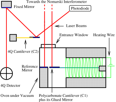
Figure 2: Experimental setup.

In Fig. 3 we plot the square root of the cantilever’s fluctuation spectral density as a function of frequency for a typical experiment at ambient temperature. The measure is compared with the FDT prediction, obtained from Eq. 10 (blue line), and the interferometer noise (red line). The measure scales quite well with the prediction. One can observe the cantilever resonance and the $1/\sqrt{\nu}$ behaviour for $\nu\ll\nu_{0}$ produced by the viscoelastic damping (see Eq. 12). However, the measurement is still too noisy in order to study accurately violations of the FDT during aging.

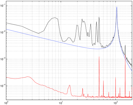
Figure 3: Square root of the fluctuation spectral density without denoising ($\textrm{nm}/\sqrt{\mathrm{Hz}}$) vs frequency (Hz).

To improve our signal-to-noise ratio we have applied our denoising technique described in Sec. 2. As already mentioned, the total cantilever displacement reads $x_{c}=x_{T}+x_{\mathrm{acc}}$. To get $x_{T}$ we have to estimate $x_{\mathrm{acc}}$. The residual acceleration of the table where the interferometer is installed is about, $10^{-8}\textrm{ m}\,\textrm{s}^{-2}$ at 1 Hz and $10^{-7}\textrm{ m}\,\textrm{s}^{-2}$ at 100 Hz. This is too small to be detected by standard accelerometers, so we used a different method. We built another cantilever made by harmonic steel (cantilever C2) which is installed very close to the Polycarbonate cantilever (cantilever C1). The parameters $\{a,b,l,m\}$ of C2 are chosen to optimize the sensitivity to mechanical vibrations and reduce its sensitivity to thermal noise (see Eq. 15). A heavy mass and a heavy mirror, that give the main contribution to $m$ for C2, are fixed on the steel cantilever free end. The cantilever C2 is damped by the viscosity of the air. A laser beam is reflected by the mirror glued on C2 and sent to a four quadrant position sensitive photodiode (4Q), which is used to detect the vibrations of the steel cantilever. The sensitivity is much smaller than that of the Nomarski interferometer, but enough for reducing the noise. Specifically, C2 is 20 mm long, 10 mm wide, 0.125 mm thick, it has a total mass of 1.3 g approximately and a resonance frequency around 20 Hz. The maximum sensitivity external acceleration of this setup, which is limited by the 4Q detector, is about $10^{-7}\textrm{ m}\,\textrm{s}^{-2}$ in the frequency range of our interest. The output signal $x_{\mathrm{4Q}}$ of the four quadrant detector and its Fourier transform $\hat{x}_{\mathrm{4Q}}$ are mainly proportional to the response of C2 to the external mechanical noise. Indeed, as we have already mentioned, thermal fluctuations of C2 are negligible. An example of the square root of the spectral density of the 4Q signal $x_{\mathrm{4Q}}$ is plotted in Fig. 4, which is related, via the response of C2, to the spectrum of the residual acceleration of the optical table. The polycarbonate cantilever and the steel cantilever, which are mounted very close on the same optical table, are perturbed by the same environmental noise sources. As theses sources may change of nature and of position, the responses of C1 and C2 to these external perturbations may change too. That is the reason why the denoising technique proposed in Sec. 2 can be very useful, because no hypothesis is needed on the response of the devices to the external noise. Referring to Sec. 2, one has to make the following substitutions: $x\rightarrow x_{c}$, $x_{\mathrm{true}}\rightarrow x_{T}$ and $x_{\mathrm{det}}\rightarrow x_{\mathrm{4Q}}$, whence

$$\langle{|\hat{x}_{T}|}^{2}\rangle = \langle{|\hat{x}_{c}|}^{2}\rangle-{|\hat{R}_{\mathrm{d}}|}^{2}\langle{|\hat{x}_{\mathrm{4Q}}|}^{2}\rangle,$$ (16)

$$\textrm{with }\hat{R}_{\mathrm{d}} = \frac{\langle\hat{x}\,\hat{x}_{\mathrm{4Q}}^{*}\rangle}{\langle{|\hat{x}_{\mathrm{4Q}}|}^{2}\rangle},$$ (17)

where the average $\langle\cdot\rangle$ is computed in our experiment on a time interval ${T}=1\textrm{ min}$, because $\hat{R}_{\mathrm{d}}$ evolves on a time scale of a few minutes. This is shown in Fig. 5 where we plot $\hat{R}_{\mathrm{d}}$, measured in three different time intervals separated by a few minutes. We see that the large variability of this response will make any a priori hypothesis useless. Using these data, we apply the denoising technique and we compute $\langle{|\hat{x}_{T}|}^{2}\rangle$ for each time interval of length ${T}$. Finally, we average the spectra obtained over several time intervals.

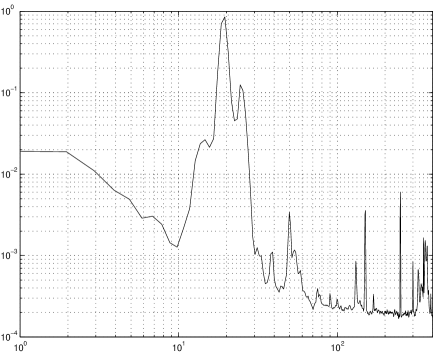
Figure 4: Square root of the spectral density of $x_{\mathrm{4Q}}$ vs frequency (Hz). This signal is related to the environmental noise.

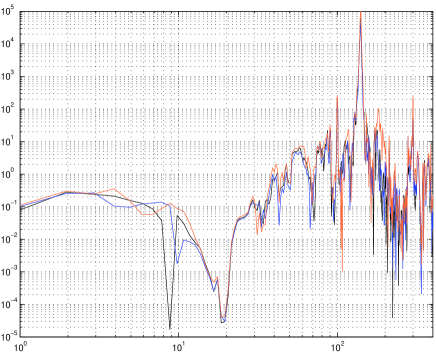
Figure 5: Example of three $|\hat{R}_{\mathrm{d}}|$ measured at different time intervals of length ${T}=1\textrm{ min}$ separated by $2\textrm{ min}$. Notice the large variation between the three curves taken at different times.

In Fig. 6 we plot $\sqrt{\langle|{\hat{x}_{T}|}^{2}\rangle}$ as obtained after having applied the noise reduction technique on twenty time intervals of length ${T}=1\textrm{ min}$. By comparing this curve with Fig. 3 we see that all the peaks have been strongly reduced and that the agreement with the FDT prediction is much better than in Fig. 3. Notice that no improvement is observed if the denoising technique is applied on a single time interval of ${T}=20\textrm{ min}$. We stress again that this effect is due to the fact that response is changing as a function of time.

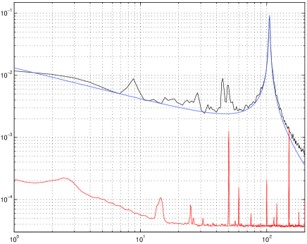
Figure 6: Square root of the fluctuation spectral density with denoising ($\textrm{nm}/\sqrt{\mathrm{Hz}}$) vs frequency (Hz).

This example clearly shows that the denoising technique proposed in Sec. 2 can reduce the influence of environmental noise on a measure if $R_{\mathrm{d}}$ is computed on short time intervals. The strong noise reduction introduced by this technique allows us to study the evolution of the FDT in an aging material. The accuracy is now limited by the 4Q noise, but this can be strongly reduced by replacing it with another Nomarski interferometer.

5 Discussion and conclusions

In this article, we have proposed an original and simple denoising technique, which allows one to reduce the influence of the environmental noise on a measure. As already mentioned, this denoising technique mixes several features of the standard feedback systems and those of the Wiener filtering. The example presented in Sec. 3 clearly shows that this technique can be very effective in suppressing spurious peaks on the spectra. The example of Sec. 3 is not exhaustive. Indeed, the same technique can be used to reduce pick-up effects in electrical measurements or eventually in very precise AFM measurements.

As a general conclusions we can say that this technique is simple and can be implemented rather easily. The only requirement is to have a reliable measurement of the environmental noise. Of course, it can be strongly improved by a multidirectional measurement of the noise.

Acknowledgements

The authors thank P. Abry, L. Bellon and I. Rabbiosi for useful discussions, and acknowledge M. Moulin, F. Ropars and F. Vittoz for technical support.

References

- [1] ETS-LINDGREN Documentation, RF Shielded Enclosures, Modular Shielding System Series (2002)
- [2] A. Papoulis, Signal Analysis, 4th printing, McGraw-Hill (1988)
- [3] J. Max, Méthodes et Techniques de Traitement du Signal et Applications aux Mesures Physiques, Tome 2, Appareillages, Méthodes Nouvelles, Exemples d’Applications, 4th edition, Masson (1987)
- [4] J. Lifermann, Les Principes du Traitement Statistique du Signal, Tome 1, Les Méthodes Classiques, Masson (1981)
- [5] R.E. Kalman, A new approach to linear filtering and prediction problems, Transactions of the ASME, Journal of Basic Engineering 82 D, 35-45 (1960)
- [6] R.E. Kalman, R.S. Bucy, New results in linear filtering and prediction theory, Transactions of the ASME, Journal of Basic Engineering 38 D, 95-108 (1961)
- [7] T.S. Grigera, N.E. Israeloff, Observation of fluctuation-dissipation-theorem violations in a structural glass, Phys. Rev. Lett. 83, 5038-5041 (1999)
- [8] L. Bellon, S. Ciliberto, Experimental study of the fluctuation dissipation during an aging process, Physica D 168-169, 325-335 (2002)
- [9] D. Hérisson, M. Ocio, Fluctuation-dissipation ratio of a spin glass in the aging regime, Phys. Rev. Lett. 88, 257702-1 - 257202-4 (2002)
- [10] L. Bellon, L. Buisson, S. Ciliberto, F. Vittoz, Zero applied stress rheometer, Rev. Sci. Instrum. 73 (9), 3286-3290 (2002)
- [11] L. Buisson, L. Bellon, S. Ciliberto, Intermittency in ageing, J. Phys.: Condens. Matter 15, S1163-S1179 (2003)
- [12] W.H. Press, S.A. Teukolsky, W. T. Vetterling, B.P. Flannery, Numerical Recipes in C. The Art of Scientific Computing, Second Edition, Cambridge University Press (1992)
- [13] L.F. Cugliandolo, J. Kurchan, L. Peliti, Energy flow, partial equilibration, and effective temperatures in systems with slow dynamics, Phys. Rev. E 55 (4), 3898-3914 (1997)
- [14] S. Fielding, P. Sollich, Observable dependence of the fluctuation dissipation relation and effective temperature, Phys. Rev. Lett. 88 (5), 050603-1 - 050603-4 (2002)
- [15] L.D. Landau, E.M. Lifshitz, Theory of Elasticity, 3rd edition, Butterworth-Heinemann (1986)
- [16] L.D. Landau, E.M. Lifshitz, Statistical Physics, Part 1, 3rd edition, Butterworth-Heinemann (1980)
- [17] N.G. McGrum, B.E. Read, G. Williams, Anelastic and Dielectric Effects in Polymeric Solids, Wiley (1967)
- [18] G. Nomarski, Microinterféromètre à ondes polarisées, J. Phys. Radium 16, 9S-16S (1954)
- [19] M. Françon, S. Mallick, Polarization Interferometers, Wiley (1971)
- [20] L. Bellon, S. Ciliberto, H. Boubaker, L. Guyon, Differential interferometry with a complex contrast, Optics Communications 207, 49-56 (2002)
- [21] G. Ballardin et al, Measurement of the VIRGO superattenuator performance for seismic noise suppression, Rev. Sci. Instrum. 72 (9), 3643-3652 (2001)
- [22] G. Losurdo et al, Inertial control of the mirror suspensions of the VIRGO interferometer for gravitational wave detection, Rev. Sci. Instrum. 72 (9), 3653-3661 (2001)
- [23] E. Coccia, V. Fafone, Noise attenuators for gravitational wave experiments, Nucl. Instr. and Meth. in Phys. Res. A 366, 395-402 (1995)
- [24] E. Puppin, V. Fratello, Vibration isolation with magnet springs, Rev. Sci. Instrum. 73 (11), 4034-4036 (2002)