Synchro-Betatron Stop-Bands due to a Single Crab Cavity

Abstract

We analyze the stop-band due to crab cavities for horizontal tunes that are either close to integers or close to half integers. The latter case is relevant for today’s electron/positron colliders. We compare this stop-band to that created by dispersion in an accelerating cavity and show that a single typical crab cavity creates larger stop-bands than a typical dispersion at an accelerating cavity.

We furthermore analyze whether it is beneficial to place the crab cavity at a position where the dispersion and its slope vanish. We find that this choice is worth while if the horizontal tune is close to a half integer, but not if it is close to an integer. Furthermore we find that stop-bands can be avoided when the horizontal tune is located at a favorable side of the integer or the half integer.

While we are here concerned with the installation of a single crab cavity in a storage ring, we show that the stop-bands can be weakened, although not eliminated, significantly when two crab cavities per ring are chosen suitably.

I Introduction

A crossing angle at the interaction region (IR) of colliding beam accelerators introduces synchro-beta responses piwinski77 ; piwinski85 . This is due to the fact that the beam-beam focusing is different for particles at different positions along the bunch, so that the horizontal beam-beam force is modulated by synchrotron oscillations of the particles. Crab cavities have been envisioned to eliminate this source so coupling for linear colliders palmer88 and circular colliders oide89 . While construction work started in early work on B-factories Padamsee:1991wv it is now planned to use crab cavities for the first time in KEK-B, in order to have bunches collide head on in IRs with crossing angle Akai:2004np . While this eliminates the synchro-beta resonances due to the beam-beam kick if the hourglass effect is negligible krishnagopal89 , it requires transverse kicks in the crab cavities that depend on the longitudinal bunch position and therefore, even in absence of beam-beam interaction, crab cavities themselves introduce synchro-beta resonances. Furthermore it has been suggested that crab cavities could be used in the damping rings of a linear collider.

Consider a storage ring that has an accelerating cavity and a crab cavity. The transport matrix $\underline{T}^{kc}$ from the accelerating cavity to the crab cavity for the phase space coordinates $x$, $x^{\prime}$, $\tau$ and $\delta$ is given by the Twiss parameters at both places and by the betatron phase advance $\phi_{kc}$ from the accelerating to the crab cavity handbook ,

$$\underline{T}^{kc} = \left(\begin{array}[]{ccc}\underline{T}^{kc}_{x}&\vec{0}&\vec{d}_{kc}\\ \vec{t}_{kc}^{T}&1&T^{kc}_{56}\\ \vec{0}^{T}&0&1\end{array}\right)\ ,$$ (4)

$$\underline{T}^{kc}_{x11} = \sqrt{\frac{\beta_{k}}{\beta_{c}}}[\cos(\phi_{kc})+\alpha_{c}\sin(\phi_{kc})]\ ,$$

$$\underline{T}^{kc}_{x12} = \sqrt{\beta_{k}\beta_{c}}\sin(\phi_{kc})\ ,$$

$$\underline{T}^{kc}_{x21} = \frac{(\alpha_{c}-\alpha_{k})\cos(\phi_{kc})-(1+\alpha_{k}\alpha_{c})\sin(\phi_{kc})}{\sqrt{\beta_{k}\beta_{c}}}\ ,$$

$$\underline{T}^{kc}_{x22} = \sqrt{\frac{\beta_{c}}{\beta_{k}}}[\cos(\phi_{kc})-\alpha_{k}\sin(\phi_{kc})]\ .$$

We use the coordinate $\tau=(t_{0}-t)\frac{E_{0}}{p_{0}}$ which is the complex conjugate to $\delta=\frac{E-E_{0}}{E_{0}}$ where $t_{0}$, $E_{0}$ and $p_{0}$ are the time of flight, the energy and the momentum of a reference particle. For highly relativistic particles $\tau=z$, the longitudinal position of the particle. If the non-periodic dispersion starts at the cavity with zero, it is $\vec{d}_{kc}=(D_{kc},D^{\prime}_{kc})^{T}$ at the crab cavity. Since the transport matrix has to be symplectic, $\vec{t}_{kc}=(T^{kc}_{51},T^{kc}_{52})^{T}$ is given by

$$\vec{t}_{kc}=-\underline{T}^{kcT}_{x}\underline{J}\vec{d}_{kc}\ .$$ (5)

The transport matrix $\underline{T}^{cc}$ from after the cavity once around the ring to just before the cavity is given by

$$\underline{T}^{cc}=\left(\begin{array}[]{ccc}T^{cc}_{x}&0&\vec{d}_{c}\\ \vec{t}_{c}^{T}&1&-2\pi R\alpha-\vec{t}_{c}^{T}\vec{\eta}_{c}\\ \vec{0}^{T}&0&1\end{array}\right)\ ,$$ (6)

where $\alpha$ is the momentum compaction factor and $2\pi R$ is the storage ring’s circumference. The periodic dispersion $\vec{\eta}_{c}=(\eta_{c},\eta^{\prime}_{c})^{T}$ at the cavity determines

$$\vec{d}_{c}=(\underline{1}-\underline{T}^{cc}_{x})\vec{\eta}_{c}\ ,$$ (7)

and symplecticity again requires

$$\vec{t}_{kc}=-\underline{T}^{ccT}_{x}\underline{J}\vec{d}_{kc}\ .$$ (8)

This leads to the term $\vec{t}_{c}^{T}\vec{\eta}_{c}=-2\pi R\alpha h_{c}\sin\mu$ with $\mu$ being the betatron phase advance per turn, and $h_{c}=\frac{1}{2\pi R\alpha}(\gamma_{c}\eta_{c}^{2}+2\alpha_{c}\eta_{c}\eta_{c}^{\prime}+\beta_{c}\eta_{c}^{{}^{\prime}2})$.

The transport matrix of the accelerating cavity is given by

$$\underline{T}_{\rm cav}=\left(\begin{array}[]{cccc}1&0&0&0\\ 0&1&0&0\\ 0&0&1&0\\ 0&0&\frac{2\sin^{2}(\frac{\mu_{s}}{2})}{\pi R\alpha}&1\end{array}\right)\ .$$ (9)

It is chosen to let the synchrotron tune be $\nu_{s}=\frac{\mu_{s}}{2\pi}$ for the case of zero dispersion at this cavity. And the matrix of the crab cavity is given by

$$\underline{T}_{\rm crab}=\left(\begin{array}[]{cccc}1&0&0&0\\ 0&1&\xi&0\\ 0&0&1&0\\ \xi&0&0&1\end{array}\right)\ .$$ (10)

The one turn matrix just after the accelerating cavity is given by $\underline{T}_{\rm cav}\underline{T}_{cc}$ when the crab cavity is switched off, and the one turn matrix just before the crab cavity is given by

$$\underline{T}_{kk}^{{\rm tot}}=\underline{T}_{kc}\underline{T}_{cav}\underline{T}_{cc}\underline{T}_{kc}^{-1}\underline{T}_{\rm crab}\ .$$ (11)

All of these matrices are symplectic.

Synchro-beta resonances are driven by either dispersion at the accelerating cavity, i.e. $\vec{\eta}_{c}\neq\vec{0}$, or by a crab cavity with $\xi\neq 0$. When $\vec{\eta}_{c}=\vec{0}$ and $\xi=0$, we have a decoupled case, and $\underline{T}_{kk}^{{\rm tot}}$ has the four eigenvalues $e^{\pm i\mu_{x,s}}$. In general the eigenvalues are determined by the characteristic equation

$${\rm Det}(\underline{T}_{kk}^{{\rm tot}}-\lambda\cdot\underline{1})=0\ ,$$ (12)

which gives

$$y^{2}+a_{1}y+a_{2}=0\ ,\ \ y=\lambda+\frac{1}{\lambda}\ .$$ (13)

Here $a_{1}$ is the coefficient for $\lambda$ in Eq. (12) and $a_{2}+2$ is the coefficient for $\lambda^{2}$.

For stability, we need all four eigenvalues $\lambda$ to have unit absolute values. This requires that (A) $y=\lambda+\frac{1}{\lambda}$ is real so that $\lambda$ is on the unit circle whenever it is complex. This condition requires

$$a_{1}^{2}-4a_{2}\geq 0\ .$$ (14)

Furthermore we require (B) $|y|<2$ so that $\lambda$ is not real. This requires

$$\pm a_{1}+\sqrt{a_{1}^{2}-4a_{2}}<4\ .$$ (15)

This amounts to two conditions depending on the sign of $a_{1}$, to which we refer as (B₊) and (B_-).

The first condition to (A) can easily be violated at first order resonances $\mu\pm\mu_{s}=2\pi n$. Synchro-beta coupling can then move two eigenvalues $\lambda$ toward each other. When two eigenvalues become close, they can move away from the unit circle of $|\lambda|=1$ in the complex plane. Since the synchrotron phase advance $\mu_{s}$ is close to 0, this condition becomes relevant when the horizontal tune $\nu=\frac{\mu}{2\pi}$ is close to an integer.

The second condition (B) becomes relevant when the horizontal tune is close to an integer or a half integer. The coupling can then move $\lambda$ to real values.

In the following we compute conditions $(A)$ and $(B)$ for the following cases:

• No crab cavity but with dispersion at the accelerating cavity, i.e. $\xi=0$ and $\vec{\eta}_{c}\neq\vec{0}$.

• No dispersion at the crab cavity and at the accelerating cavity, i.e. $\xi\neq 0$, $\vec{\eta}_{k}=\vec{0}$ and $\vec{\eta}_{c}=\vec{0}$.

• Dispersion at the crab cavity but no dispersion at the accelerating cavity, i.e. $\xi\neq 0$, $\vec{\eta}_{k}\neq\vec{0}$ and $\vec{\eta}_{c}=\vec{0}$.

Case B is a special case of case C.

We will evaluate the stop-bands that occur close to integer and half-integer values of the horizontal tune $\nu$ due to condition (A) and (B) respectively. As an example we will use the parameters of Tab. 1 unless specified otherwise. Typically the crab cavity strength is given by the half crossing angle $\phi$ at the interaction point via

$$\xi=\frac{2\phi}{\sqrt{\beta_{k}\beta_{x}^{*}}}\ ,$$ (16)

where $\beta_{x}^{*}$ is the horizontal $\beta$ function at the interaction point. The range of the crab cavity strength used in the following examples is $\xi\in[0,0.03]\frac{1}{{\rm m}}$. This range is motivated by a crossing angle of about $\phi=30$mrad and beta functions of about $\beta_{k}=50$m and $\beta_{x}^{*}=0.02$m. The range of synchrotron tunes used in the following examples is $\mu_{s}\in[-0.1,0.1]$.

$\eta_{k}$

=

10m

, $\eta_{c}$

=

10m

, $\eta^{\prime}_{k}$

=

0

, $\eta^{\prime}_{c}$

=

0

,

$\beta_{k}$

=

10m

, $\alpha_{k}$

=

0

, $\beta_{c}$

=

10m

, $\alpha_{c}$

=

0

,

$\alpha$

=

0.01

, $R$

=

100m

, $T_{56}^{kc}$

=

0

.

Table 1: Parameters for the stop-band examples. The numbers for the dispersion apply in all examples where they are not specified otherwise.

I.1 No crab cavity

For $\xi=0$ and $\vec{\eta}_{c}\neq\vec{0}$, the coefficients $a_{1}$ and $a_{2}$ come out to be

$$a_{1}^{A} = -2(\cos\mu+\cos\mu_{s}+2h_{c}\sin\mu\sin^{2}\frac{\mu_{s}}{2})\ ,$$ (17)

$$a_{2}^{A} = 4(\cos\mu\cos\mu_{s}+2h_{c}\sin\mu\sin^{2}\frac{\mu_{s}}{2})\ .$$ (18)

Since there is no crab cavity, the eigenvalues do not depend on the Twiss parameters or phase advances with index $k$.

I.2 No dispersion at both cavities

The transport matrix for one turn that starts just before the crab cavity depends on the phase advance between the accelerating and the crab cavity and also on the time of flight term $T^{kc}_{56}$ between these locations. We express this term relative to the momentum compaction as $r_{56}=\frac{T^{kc}_{56}}{2\pi R\alpha}$. For $\xi\neq 0$ and $\vec{\eta}_{k}=\vec{\eta}_{c}=\vec{0}$, the coefficients $a_{1}$ and $a_{2}$ come out to be

$$a_{1}^{B} = -2(\cos\mu+\cos\mu_{s})\ ,$$ (19)

$$a_{2}^{B} = 4\{\cos\mu\cos\mu_{s}$$

$$+ \xi^{2}\beta_{k}\sin\mu\frac{\pi R\alpha}{2}[1+4r_{56}(1+r_{56})\sin^{2}\frac{\mu_{s}}{2}]\}\ .$$

It is interesting to note that the eigenvalues do not depend on the phase advance between the cavities.

I.3 Dispersion at a crab cavity

When there is a crab cavity, we want to analyze the leading order effect, which is second order in the perturbations $\eta_{k}$, $\eta^{\prime}_{k}$, and $\xi$. For $\xi\neq 0$, $\vec{\eta}_{k}\neq\vec{0}$, $a_{1}$ and $a_{2}$ come out to be

$$a_{1}^{C} = a_{1}^{B}+4\xi\eta_{k}(1+2r_{56})\sin^{2}\frac{\mu_{s}}{2}+2\xi g_{k}\sin\mu\ ,$$ (21)

$$a_{2}^{C} = a_{2}^{B}-8\xi[(1+r_{56})\eta_{k}\cos\mu\sin^{2}\frac{\mu_{s}}{2}+\frac{g_{k}}{2}\sin\mu\cos\mu_{s}]$$ (22)

$$+ 2\xi^{2}\{\eta_{k}^{2}(\cos\mu\cos\mu_{s}-1)$$

$$+ 2\eta_{k}[g_{k}(1+2r_{56})+h_{k}\eta_{k})\sin\mu\sin^{2}\frac{\mu_{s}}{2}]\}\ .$$

Here the short form $g_{k}=\alpha_{k}\eta_{k}+\beta_{k}\eta^{\prime}_{k}$ and $h_{k}=\frac{1}{2\pi R\alpha}(\gamma_{k}\eta_{k}^{2}+2\alpha_{k}\eta_{k}\eta_{k}^{\prime}+\beta_{k}\eta_{k}^{{}^{\prime}2})$ were used.

II Horizontal Tune Close to Integers

Condition (A) is relevant when the horizontal phase advance is close to a given synchrotron phase advance $\mu_{s}$, which is usually much smaller than $2\pi$, this equation leads to a stop-band for the horizontal tune $\nu=\frac{\mu}{2\pi}$ close to every integer. The boundary of stability is found by solving

$$a_{1}^{2}-4a_{2}=0$$ (23)

for $\mu_{s}$.

One additionally has to check whether condition (B) is satisfied in the regions which are declared as stable. For the parameters chosen here, this is the case.

II.1 No crab cavity

For $\xi=0$, Eqs. (17) and (18) for $a_{1}^{A}$ and $a_{2}^{A}$ lead to

$$\cos\mu_{s} = \frac{1}{(1-h_{c}\sin\mu)^{2}}(\pm 4\sin^{2}\frac{\mu}{2}\sqrt{h_{c}\sin\mu}$$ (24)

$$+ \cos\mu-h_{c}(3-\cos\mu-h_{c}\sin\mu)\sin\mu)\ .$$ (25)

At the stop-band $\mu$ is close to $\mu_{s}$, which is usually small, and we therefore expand to second order in the fractional part $\delta\nu\in[-\frac{1}{2},\frac{1}{2}]$ of the horizontal tune $\nu=\frac{\mu}{2\pi}$ leading to the approximate location of the stop-band at

$$\mu_{s}=\pm(\delta\mu+h_{c}\sin^{2}\mu)$$ (26)

and to the width of the stop-band

$$\Delta\mu_{s}=\pm\sqrt{h_{c}}\sin^{\frac{3}{2}}\mu\ .$$ (27)

Note that this only leads to a real stop-band width when $\nu$ is slightly above an integer. Here and in all subsequent statements we assume that the energy is above transition, i.e. $\alpha>0$. Note that the synchrotron tune above transition is negative. However, all subsequent formulas depend on $\cos\mu_{s}$ only so that the sign of the synchrotron tune does not matter.

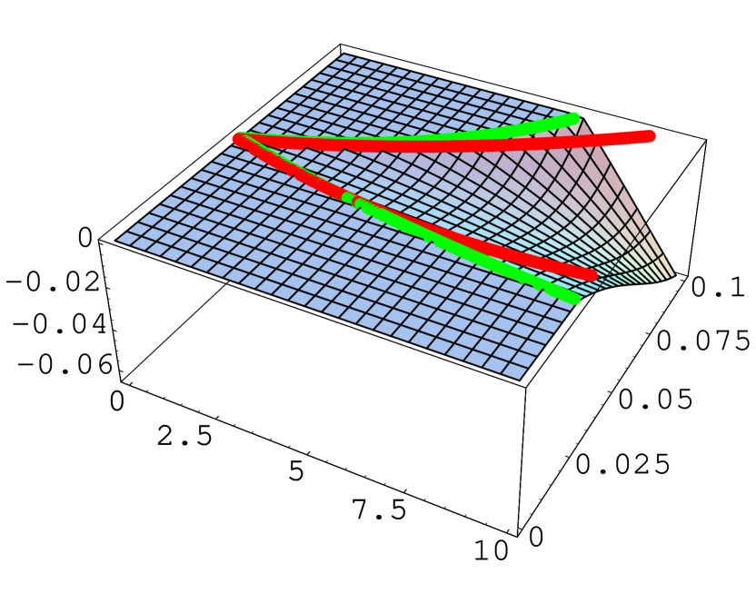
Figure 1: Unstable region caused by dispersion at a cavity for $\nu$ close to an integer. Light green: border of stability. Dark red: border of stability from the approximate Eq. 27.

Figure 1 shows the unstable region caused by dispersion in a cavity. The parameters of Tab. 1 were used. The valley of instability shows $a_{1}^{2}-4a_{2}$ in the region where it is negative, i.e.  the stability function $s_{A}(a_{1},a_{2})={\rm Min}(a_{1}^{2}-4a_{2},0)$ is plotted. The light green line indicates the border of stability computed by Eq. (25). The approximation in Eq. (27) leads to the dark red curve. It is apparent that the approximation is very good for $\eta<5$m.

II.2 No dispersion at both cavities

For $\xi\neq 0$, $\vec{\eta}_{c}=\vec{\eta}_{k}=\vec{0}$ we obtain from Eqs. (19) and (I.2) for $a_{1}^{B}$ and $a_{2}^{B}$ an equation for the boundary of instability for $\cos\mu_{s}$. For the example of $r_{56}=0$ it is

$$\cos\mu_{s}=\pm\cos\mu\pm\xi\sqrt{2\pi R\alpha_{k}\beta_{k}\sin\mu}\ .$$ (28)

To leading order in $\xi$ one obtains the approximate location and width of the stop-band,

$$\mu_{s} = \pm\delta\mu\ ,$$ (29)

$$\Delta\mu_{s} = \pm\xi\sqrt{\frac{2\pi R\alpha\beta_{k}}{\sin\mu}}\sqrt{1+4r_{56}(1+r_{56})\sin^{2}\frac{\mu}{2}}\ .$$ (30)

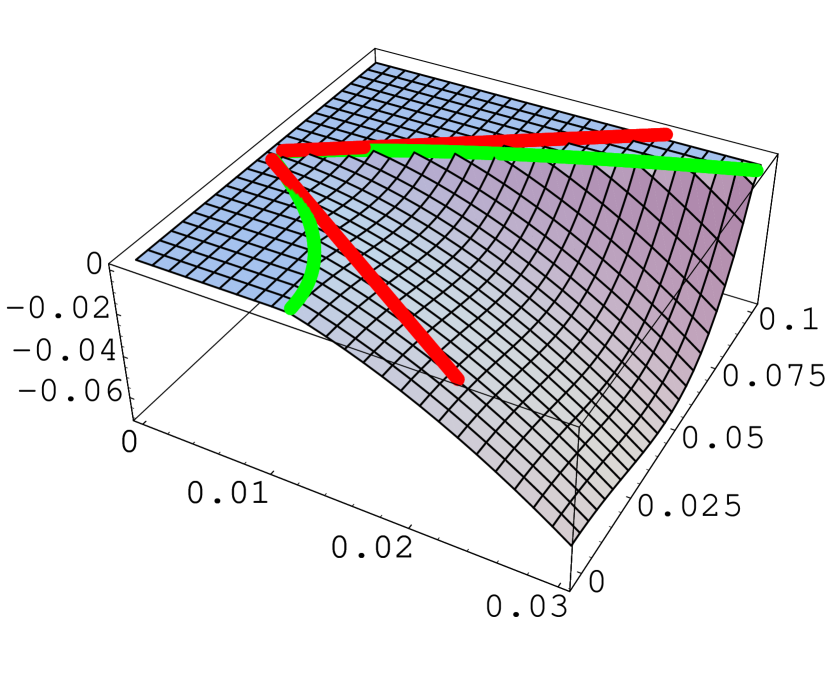
Figure 2: Unstable region caused by a crab cavity. Light green: border of stability, Dark Red: approximation to this border.

Figure 2 shows the unstable region. Again the light green curves show the border of stability and the dark red curves indicate the approximation of Eq.(30), which apparently is very good for $\xi<0.007\frac{1}{{\rm m}}$.

II.3 Dispersion at a crab cavity

If the dispersion in the crab cavity is not matched to a small value, it will typically be as large as several meters. Since this is not a small perturbation, we only linearize in $\xi$ and in $\delta\mu$.

When using Eqs. (21) and (22) for solving $a_{1}^{C2}-4a_{2}^{C}=0$ for $\mu_{s}$ and subsequently linearizes in $\xi$ and $\delta\mu$ one obtains

$$\mu_{s}=\pm\{\delta\mu+\xi[g_{k}-\eta_{k}(1+2r_{56})\frac{\sin\mu}{2}]\}\ .$$ (31)

For the width of the stop-band one obtains

$$\Delta\mu_{s}=\pm\xi\sqrt{\frac{2\pi R\alpha\beta_{k}}{\sin\mu}}(1-\frac{\eta_{k}^{2}}{2\pi R\alpha\beta_{k}}\sin\mu)\ .$$ (32)

It is interesting that no real stop-band width exists when $\sin\mu$ is negative, and the stop-band only occurs above integer horizontal tunes. Higher order terms of the stop-band width expansion depend on the time of flight term $r_{56}$, $\alpha_{k}$ and $\eta^{\prime}_{k}$.

Now we can evaluate whether dispersion at the crab cavity has a negative influence on the stop-band width. Since there is only a stop-band for $\sin\mu>0$, it turns out that in Eq. (32) a dispersion at the crab cavity reduces the stop-band width, as long as $\eta_{k}^{2}$ is smaller than $\frac{2\pi R\alpha\beta_{k}}{\sin\mu}$.

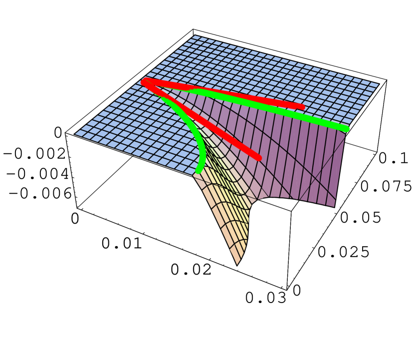
Figure 3: Unstable region caused by a crab cavity for a horizontal slightly above an integer. Top: $\eta_{k}=11$m, Bottom: $\eta_{k}=14.32$m. Light green: border of stability. Dark red: border of stability from the approximate Eq. 32.

Figure 3 (bottom) shows the unstable region bordered by a light green curve for the optimal value of $\eta_{k}=\sqrt{\frac{2\pi R\alpha\beta_{k}}{\sin\mu}}=14.32$m. The approximate Eq. (32) indicated by the dark red curve evaluates to zero stop-band width for this dispersion. In fact, the stop-band is extremely narrow but due to higher order terms it does not have zero width. But Fig. 3 (top) for $\eta_{k}=11$m shows that the approximation works quite reliably for non-optimal dispersions.

The other parameters were chosen as specified in Tab. 1. It is evident that the dispersion reduces the width of the stop-band greatly, and it could be recommended to use the dispersion at the crab cavity to reduce the stop-band width. However, the B-factories at SLAC and KEK as well as other $e^{+}/e^{-}$ colliders like CESR have horizontal tunes which are close to a half integer and therefore the subsequent section about stop-bands at half-integer tunes is more relevant for these applications.

III Horizontal Tune Close to Half Integers

When using condition (A) for determining stability, one additionally has to check whether condition (B) is satisfied in the regions which are declared stable by condition (A). For the parameters of the examples shown above, this is the case. When, as in the case of the B-factories or other $e^{+}/e^{-}$ colliders the horizontal tune is close to a half integer, whereas the synchrotron tune is small, the coupling strength will not bring two eigenvalues $\lambda$ together. It can however happen that one of the eigenvalues becomes real, and it is here that condition (B) becomes important. In the following examples we therefore use $\nu=8.49$ or $\nu=8.51$.

The borders of stability are found by solving

$$\pm a_{1}+\sqrt{a_{1}^{2}+2a_{2}}=4$$ (33)

for $\mu_{s}$.

III.1 No crab cavity

Using the coefficients $a_{1}^{A}$ and $a_{2}^{A}$ from Eqs. (17) and (18), Eq. 33 yields the border of stability, and for $a_{1}^{A}>0$ one obtains

$$\cos\mu_{s}=-\frac{\cos\frac{\mu}{2}+2h_{c}\sin\frac{\mu}{2}}{\cos\frac{\mu}{2}-2h_{c}\sin\frac{\mu}{2}}\ .$$ (34)

For small dispersion at the cavity one obtains $\cos\mu_{s}\approx-1-4\tan\frac{\mu}{2}$, which cannot be satisfied for small synchrotron tunes. For $a_{1}^{A}<0$ one obtains only $\cos\mu_{s}=1$ so that there is no unstable region close to half-integer tunes due to dispersion at an accelerating cavity.

III.2 No dispersion at both cavities

From $a_{1}^{B}$ and $a_{2}^{B}$ in Eqs. (19) and (I.2) we obtain

$$\cos\mu_{s}=1+\xi^{2}\frac{1}{2}\pi R\alpha\beta_{k}\cot\frac{\mu}{2}\ .$$ (35)

To first order in $\xi$ this leads to a resonance at $\mu_{s}=0$ of width

$$\Delta\mu_{s}=\pm\xi\sqrt{-\pi R\alpha\beta_{k}\cot\frac{\mu}{2}}\ .$$ (36)

The stop-band in $\mu_{s}$ thus only appears when the horizontal tune is slightly above the half integer. An expansion to higher orders depends on $r_{56}$, $\alpha_{n}$ and $\eta^{\prime}_{k}$.

In Fig. 4 the valley of instability is shown by plotting $s_{B}(a_{1},a_{2})={\rm Min}(4-|a_{1}|-\sqrt{a_{1}^{2}-4a_{2}},0)$ for $\nu=8.51$. The approximation in Eq. (36) is shown together with the stop-band region. The agreement is very good. Note that the range of $\nu_{s}$ is reduced by a factor of 10 from compared to other graphs. Here the forbidden region is up to 0.01 in tune space. This is currently not critical for the B-factories but could in the future restrict the possibilities of moving the horizontal tune even closer to the half integer in B-factories.

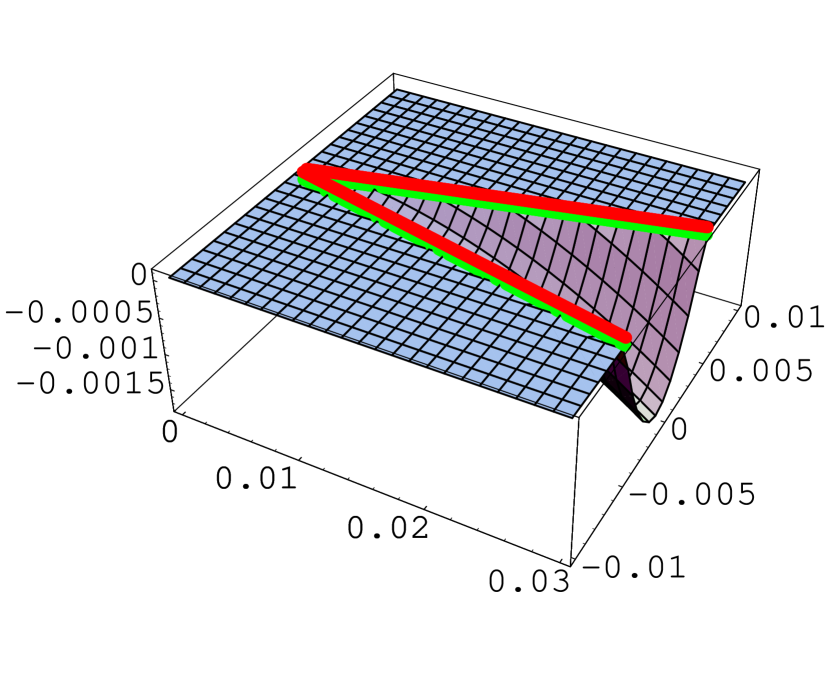
Figure 4: Unstable region caused by a crab cavity for small distances $\delta\nu$ above a half-integer tune. Light green: border of stability.

III.3 Dispersion at a crab cavity

Using $a_{1}^{C}$ and $a_{2}^{C}$ in Eqs. (21) and (22) to find the border of stability for $\mu_{s}$, and then linearizing in $\xi$ leads to the stop-band width

$$\Delta\mu_{s}=\pm\xi\sqrt{\eta_{k}^{2}-\pi R\alpha\beta_{k}\cot\frac{\mu}{2}}$$ (37)

and the stop-bands center at $\mu_{s}=0$. This result comes from the condition (B_-), $-a_{1}^{C}+\sqrt{a_{1}^{2C}-4a_{2}^{C2}}=4$, since the condition (B₊) requires $\nu_{s}=0.5$ for $\xi=0$. Higher order expansions again depend on $r_{56}$, $\alpha_{k}$ and $\eta^{\prime}_{k}$.

Equation (37) indicates that for tunes where there is a stop-band in the case of $\eta_{k}=0$, i.e. for $\nu$ above a half integer where $\cot\frac{\mu}{2}<0$, the stop-band becomes wider by introducing dispersion at the crab cavity. Furthermore, there is now also a stop-band at tunes below a half integer where $\cot\frac{\mu}{2}>0$ when the dispersion is large enough.

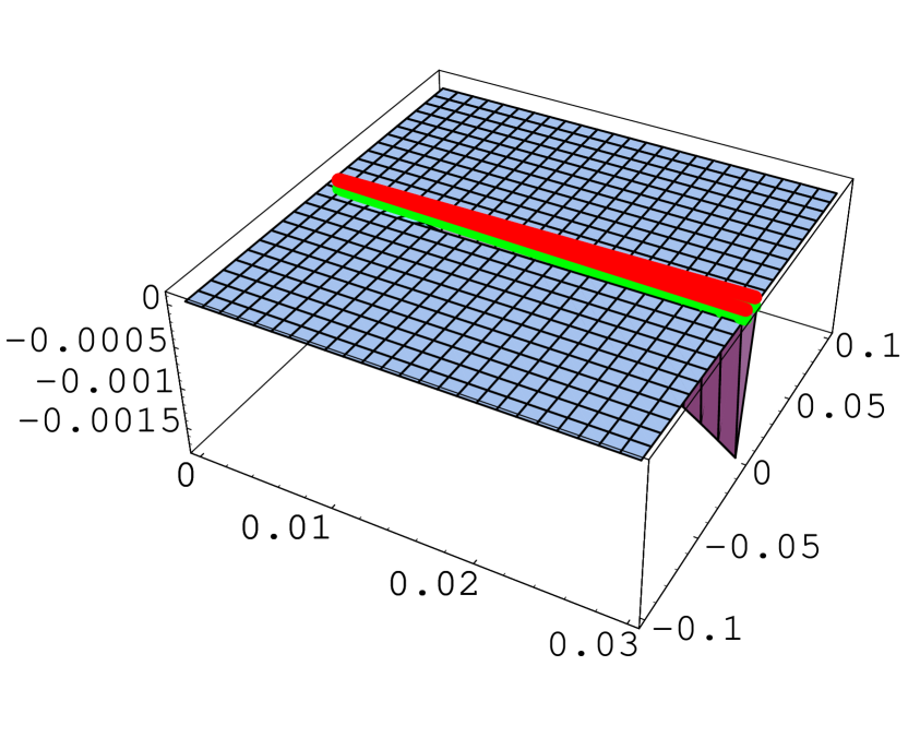
Figure 5: Unstable region caused by a crab cavity for $\nu$ close to a half integer with $\cot\frac{\mu}{2}<0$. Left: $\eta_{k}=0$, Right: $\eta_{k}=4$m. Light green: border of stability. Dark red: border of stability from the approximate Eq. 37.

Figure 5 shows the unstable region for $\mu_{s}$ with $\eta_{k}=0$ (left) and $\eta_{k}=4$m (right) for a tune of $\nu=8.51$ where $\cot\frac{\mu}{2}<0$. Especially for larger values of $\xi$ the difference is very clear. It is even clearer when investigating the unstable region for a tune of $\nu=8.49$ in Fig. 6. For $\eta_{k}=0$ (left) there is no stop-band while for $\eta_{k}=4$m (right) the stop-band is substantial.

The border of stability has two sections, one is well approximated by Eq. (37) and one is not. The former one comes from condition (B_-) on which Eq. (37) is based and the latter one comes from condition (B₊).

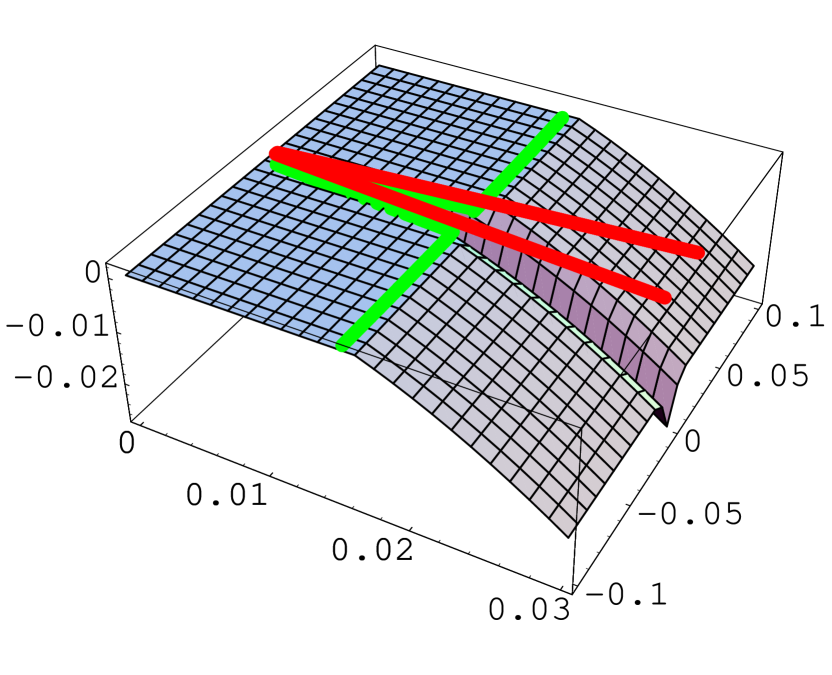
Figure 6: Unstable region caused by a crab cavity for $\nu$ close to a half integer with $\cot\frac{\mu}{2}>0$. Left: $\eta_{k}=0$, Right: $\eta_{k}=4$m. Light green: border of stability. Dark red: border of stability from the approximate Eq. 37.

The strength of this effect is nicely seen for a dispersion of only $\eta_{k}=1$m when plotting the stop-band of the horizontal tune $\nu$ for a fixed synchrotron tune of $\nu_{s}=\frac{\mu_{s}}{2\pi}=0.1$ in Fig. 7. For $\eta_{k}=0$ (top) the stop-band is located only on one side of the half integer. For $\eta_{k}=1$m (bottom) the $\nu_{s}$ stop-band is not only much wider, it also extends to both sides of the half integer.

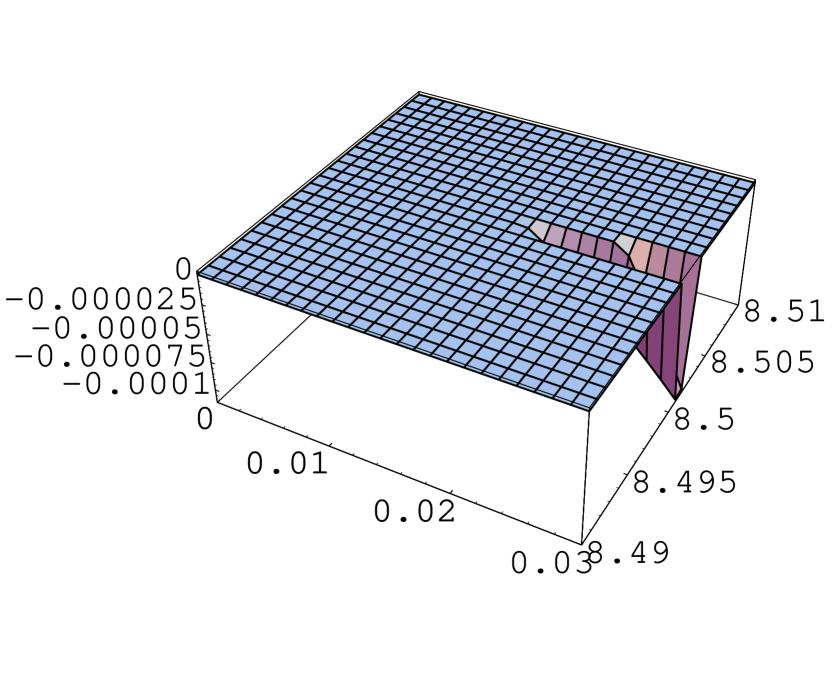
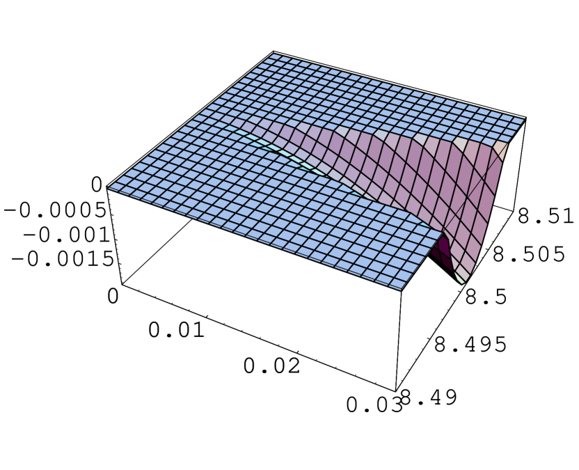
Figure 7: Unstable region caused by a crab cavity for $\nu_{s}=0.1$. Top: $\eta_{k}=0$, Bottom: $\eta_{k}=1$m. Light green: border of stability. Dark red: border of stability from the approximate Eq. 37.

IV A pair of crab cavities

While we here want to restrict ourselves to the proposed insertion of one crab cavity in a ring, it should be pointed out that a pair of crab cavities can strongly reduce the width of the stop-bands when the two crab cavities have betatron phases which differ by odd multiples of $\pi$. While this would cancel the first order synchro-beta coupling of the crab cavity exactly when the time of flight term $m_{56}$ between them vanishes, the beam-beam focusing at the interaction point will spoil this exact cancellation to some extent.

It can be shown that, when a beam-beam focusing is included at the IP, the effect can be represented as a single kick at the entrance crab cavity by a matrix

$$T_{\rm crab}=\underline{1}+4\pi\Delta\nu\beta_{k}\left(\begin{array}[]{cccc}0&1&\xi&0\\ 0&0&0&0\\ 0&0&0&0\\ 0&-\xi&-\xi^{2}&0\end{array}\right)$$ (38)

where $\Delta\nu$ is the beam-beam tune shift parameter, and $m_{56}=0$ was assumed for the transport matrix between the cavities. Furthermore we assumed $\vec{\eta}_{k}=\vec{0}$ and $\alpha_{k}=0$. As it should, when $\Delta\nu=0$, the two crab cavities have perfect cancellation and this matrix becomes a unit matrix.

The analysis can now be repeated with this new matrix for the crab cavity. It is found that the stop-band is relatively narrow. For the above numerical example with $\xi\neq 0$, $\vec{\eta}_{c}=\vec{\eta}_{k}=\vec{0}$ and $\nu=8.025$ the unstable region is shown in Fig. 8 for $\Delta\nu=0.05$. Note that the stop-band is narrower and that the unstable valley is shallower than in the corresponding Fig. 2.

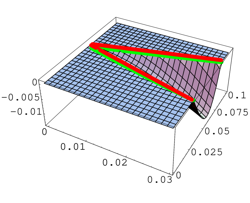
Figure 8: Unstable region caused by two crab cavities, $\pi$ apart in betatron phase for $\nu=8.025$. Light green: border of stability. Dark red: border of stability from the approximate Eq. IV.

The width of the stop-band at $\mu\pm\mu_{s}=n2\pi$ with a pair of crab cavities, for the case when there is no dispersion at the crab cavities and at the accelerating cavity, is given by

$$\mu_{s} = \pm(\delta\mu+2\pi\Delta\nu)\ ,$$ (39)

$$\Delta\mu_{s} = \pm\xi\Delta\nu 4\pi$$

$$\times \sqrt{\frac{2\pi R\alpha\beta_{k}}{\sin\mu}}\sqrt{1+4r_{56}(1+r_{56}\sin^{2}\frac{\mu}{2})}$$

which is a factor $4\pi\Delta\nu$ smaller than that due to a single crab cavity in Eq. (30). Note however that $\Delta\nu$ may become larger than $0.05$ in high luminosity operations. Again, the resonance only appears above the integer.

When the tune is close to a half integer, the border of stability for $\mu_{s}$ becomes

$$\Delta\mu_{s}=\pm\xi\sqrt{4\pi\Delta\nu}\sqrt{2\pi R\alpha\beta_{k}}\ .$$ (41)

This differs from the corresponding Eq.(36) approximately by the factor $2\sqrt{\frac{4\pi\Delta\nu}{\delta\mu}}$. An example for $\nu=8.51$ is given in Fig. 9. For the example of $\Delta\nu=0.05$ and $\delta\nu=0.01$, the valley of instability is wider and deeper than in the corresponding Fig. 4.

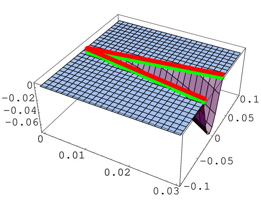
Figure 9: Unstable region caused by two crab cavities, $\pi$ apart in betatron phase for $\nu=8.51$. Light green: border of stability. Dark red: border of stability from the approximate Eq. 41.

V Conclusion

The linear synchro-beta coupling effects have been analyzed for a storage ring with a crab cavity or a crab cavity pair. When one crab cavity is to be installed in a storage ring, the dispersion at the crab cavity can be non-zero or can even be used to reduce synchro-beta stop-bands. When the tune is close to a half integer, the dispersion should be matched to a small value at the crab cavity however. In both cases it should be noted that the stop-band due to synchro-beta coupling is larger than that due to a large dispersion at an accelerating cavity. This effect can be reduced when two crab cavities are used. The advantage is limited, however, when the ring is operated with a large beam-beam tune shift.

References

- (1) A. Piwinski, IEEE Trans. on Nucl. Sci. NS-24, 1480 (1977)
- (2) A. Piwinski, IEEE Trans. on Nucl. Sci. NS-32, 2240 (1985)
- (3) R. Palmer, SLAC-PUB-4707 (1988)
- (4) K. Oide and K. Yokoya, Phys. Rev. A40, 315 (1989)
- (5) H. Padamsee, P. Barnes, C. Chen, J. Kirchgessner, D. Moffat, D. Rubin, Y. Samed, J. Sears, Q.S. Shu, M. Tigner, D. Zu, CLNS-91-1075, Cornell and Proceedings PAC91, San Francisco/CA (1991)
- (6) K. Akai and Y. Morita, Report KEK-PREPRINT-2003-123 (2003)
- (7) S. Krishnagopal and R. Siemann, CLNS 89/967, Cornell (1989)
- (8) Handboodk of Accelerator Physics and Engeneering, p. 51, Editors A. W. Chao, M. Tigner, Word Scientific Publishing Co. Pte. Ltd. (2002)