Strength of Higher-Order Spin-Orbit Resonances

Abstract

When polarized particles are accelerated in a synchrotron, the spin precession can be periodically driven by Fourier components of the electromagnetic fields through which the particles travel. This leads to resonant perturbations when the spin-precession frequency is close to a linear combination of the orbital frequencies. When such resonance conditions are crossed, partial depolarization or spin flip can occur. The amount of polarization that survives after resonance crossing is a function of the resonance strength and the crossing speed. This function is commonly called the Froissart-Stora formula. It is very useful for predicting the amount of polarization after an acceleration cycle of a synchrotron or for computing the required speed of the acceleration cycle to maintain a required amount of polarization. However, the resonance strength could in general only be computed for first-order resonances and for synchrotron sidebands. When Siberian Snakes adjust the spin tune to be $\frac{1}{2}$, as is required for high energy accelerators, first-order resonances do not appear and higher-order resonances become dominant. Here we will introduce the strength of a higher-order spin-orbit resonance, and also present an efficient method of computing it. Several tracking examples will show that the so computed resonance strength can indeed be used in the Froissart-Stora formula. HERA-p is used for these examples which demonstrate that our results are very relevant for existing accelerators.

I Introduction

In this paper we want to introduce the strength of higher-order spin orbit resonances which we want to use in the Froissart-Stora formula to compute how much polarization is lost when a resonance is crossed. For first-order resonances the definition and computation of the resonance strength is relatively simple courant80 ; hoffstaetter99i , for higher-order resonances it is much more elaborate. We will need to use the invariant spin field, also called the $\vec{n}$-axis derbenev72 , the amplitude dependent spin tune and the periodic coordinate system over phase space that determines the spin tune yokoya86a . These concepts are therefore quickly reviewed in this introduction.

While a polarized particle moves along the azimuth $\theta=\frac{2\pi l}{L}$ of the storage ring’s closed orbit with path length $l$ and total length $L$, its semi-classical spin precesses according to the T-BMT equation thomas27 ; bargmann59

$$\frac{\text{d}}{\text{d}\theta}\vec{S}=\vec{\Omega}_{0}(\theta)\times\vec{S}\ .$$ (1)

The spin direction that is periodic after one turn is referred to as $\vec{n}_{0}(\theta)$. If the spin has any other direction, it precesses around $\vec{n}_{0}$. The numbers of precessions that occur during one turn is referred to as the closed orbit spin tune $\nu_{0}$. To describe the precession, a right handed system of orthogonal unit vectors $(\vec{m},\vec{l},\vec{n}_{0})$ is introduced for any azimuth. The two vectors $\vec{l}(\theta)$ and $\vec{m}(\theta)$ precess around $\vec{n}_{0}$ according to the T-BMT equation so that they would have rotated $\nu_{0}$ times after one turn. However a precession is added that continuously winds back $\nu_{0}$ precessions. These vectors are therefore periodic in the azimuth and

$$\frac{\text{d}}{\text{d}\theta}\vec{m} = (\vec{\Omega}_{0}-\nu_{0}\vec{n}_{0})\times\vec{m}\ ,$$ (2)

$$\frac{\text{d}}{\text{d}\theta}\vec{l} = (\vec{\Omega}_{0}-\nu_{0}\vec{n}_{0})\times\vec{l}\ .$$ (3)

Since particles on the closed orbit have spins that precess around $\vec{n}_{0}$, the product $s_{3}=\vec{S}(\theta)\cdot\vec{n}_{0}(\theta)$ is an invariant, i.e. does not depend on $\theta$. It can be shown that it is also an adiabatic invariant hoffstaetter00 ; hoffstaetter02a ; neistadt75 , i.e. it hardly changes when parameters of the system, like the storage energy, are slowly changed.

This concept of an invariant spin direction, a spin tune, a periodic system of unit vectors and an adiabatic invariant can be extended to particles that do not move on the closed orbit but oscillate around this orbit and whose motion is thus described by phase space trajectories $\vec{z}(\theta)$. The T-BMT equation for spin motion then depends on the phase space trajectory

$$\frac{\text{d}}{\text{d}\theta}\vec{S}=\vec{\Omega}(\vec{z},\theta)\times\vec{S}\ .$$ (4)

If the vector field $\vec{f}(\vec{z},\theta)$ with $|\vec{f}|=1$ describes the spin distribution in a particle beam, it is called a spin field and satisfies the T-BMT equation

$$\frac{\text{d}}{\text{d}\theta}\vec{f}(\vec{z}(\theta),\theta)=\vec{\Omega}(\vec{z},\theta)\times\vec{f}\ .$$ (5)

A special spin field that is periodic from turn to turn is called the invariant spin field $\vec{n}$,

$$\vec{n}(\vec{z},\theta+2\pi)=\vec{n}(\vec{z},\theta)\ .$$ (6)

Particles that travel along the trajectory $\vec{z}(\theta)$ have spins that precess around $\vec{n}(\vec{z}(\theta),\theta)$. Describing this precession and even the number of precessions in one turn starting at $\vec{z}(\theta_{0})$ is not trivial, since the particle has a new phase space point $\vec{z}(\theta_{0}+2\pi)$ after one turn. An orthogonal set of unit vectors $(\vec{u}_{1},\vec{u}_{2},\vec{n})$ has to be defined for each phase space point and for each azimuth to determine spin precession angles.

If the unit vectors $\vec{u}_{1}$ and $\vec{u}_{2}$ would satisfy the T-BMT equation along each phase space trajectory starting at $\vec{z}_{i}$ and ending at $\vec{z}_{f}$ after one turn, these vectors would precess around $\vec{n}$ and after one turn $\vec{u}_{i}(\vec{z}_{f},\theta_{0}+2\pi)$ would have some angle $2\pi\tilde{\nu}(\vec{z}_{0})$ with respect to the initial unit vectors $\vec{u}_{i}(\vec{z}_{f},\theta_{0})$ at the same phase space point.

The rotation angle $2\pi\tilde{\nu}$ is not well defined, since the direction of the $\vec{u}_{i}$ before and after the turn is only required to be perpendicular to $\vec{n}$, but has a free angular orientation in the orthogonal plain. This free orientation for each phase space point can (under certain general conditions hoffstaetter00 ; vogt00 ; BEH04 ) be chosen to make the number of rotations $\nu$ independent of the orbital phase variables $\vec{\Phi}$. It then only depends on the amplitudes $\vec{J}$ of the orbital motion and is therefore called the amplitude dependent spin tune $\nu(\vec{J})$.

To obtain a periodic set of unit vectors, the described precession of the unit vectors is again augmented by continuously winding back $\nu$ spin precessions during one turn,

$$\frac{\text{d}}{\text{d}\theta}\vec{u}_{i}(\vec{z}(\theta),\theta)=[\vec{\Omega}(\vec{z},\theta)-\nu(\vec{J})\vec{n}(\vec{z},\theta)]\times\vec{u}_{i}\ .$$ (7)

Since spins precess around $\vec{n}$, the product $J_{S}=\vec{S}(\theta)\cdot\vec{n}(\vec{z}(\theta),\theta)$ is an invariant of motion, i.e. it does not change with $\theta$. It can be shown, however, that it is also an adiabatic invariant hoffstaetter00 ; hoffstaetter02a ; neistadt76 , i.e. it hardly changes when system parameters like the storage energy change sufficiently slowly. This has strong implications. When a beam is polarized parallel to the invariant spin field $\vec{n}(\vec{z},E_{i})$ at some initial energy $E_{i}$ and the storage energy is increased slowly, the beam will be polarized parallel to $\vec{n}(\vec{z},E_{f})$ at the final energy $E_{f}$.

This is a very important property since a beam in such a polarization state will have the average polarization $P_{\mathrm{l}im}=<\vec{n}>$ after acceleration, which can be large even if this average polarization is small at intermediate energies.

II The Single Resonance Model (SRM)

II.1 Fourier Expansion of Spin Perturbations

The quantities $\vec{n}$, $\nu$, $\vec{u}_{1}$, $\vec{u}_{2}$ and $J_{S}$ will be computed for an analytically solvable model and the adiabatic invariance will be illustrated by letting a parameter of this model change. Since this model leads to the Froissart-Stora formula, a comparison of its equations with the equations of general spin dynamics leads to the introduction of higher-order resonance strengths that can be used in the Froissart-Stora formula.

The spin precession vector for particles which oscillate around the closed orbit can be decomposed into the closed-orbit contribution $\vec{\Omega}_{0}$ and a part $\vec{\omega}$ due to the particles’ oscillations, $\vec{\Omega}(\vec{z},\theta)=\vec{\Omega}_{0}(\theta)+\vec{\omega}(\vec{z},\theta)$. In the $(\vec{m},\vec{l},\vec{n}_{0})$ system we write

$$\vec{S}=s_{1}\vec{m}+s_{2}\vec{l}+s_{3}\vec{n}_{0}\;,\ \ \vec{\omega}=\omega_{1}\vec{m}+\omega_{2}\vec{l}+\omega_{3}\vec{n}_{0}\ .$$ (8)

With the complex notation $\hat{s}=s_{1}+\text{i}s_{2}$ and $\omega=\omega_{1}+\text{i}\omega_{2}$, the equation of spin motion is

$$\vec{\Omega}\times\vec{S}=\vec{m}\frac{\text{d}}{\text{d}\theta}s_{1}+\vec{l}\frac{\text{d}}{\text{d}\theta}s_{2}+\vec{n}_{0}\frac{\text{d}}{\text{d}\theta}s_{3}+(\vec{\Omega}_{0}-\nu_{0}\vec{n}_{0})\times\vec{S}$$ (9)

and the equation of motion for $\hat{s}$ is obtained by multiplication with $\vec{m}+\text{i}\vec{l}$, and taking into account that $s_{3}=\sqrt{1-|\hat{s}|^{2}}$,

$$\frac{\text{d}}{\text{d}\theta}\hat{s}=i(\nu_{0}+\omega_{3})\hat{s}-\text{i}\omega\sqrt{1-|\hat{s}|^{2}}\;.$$ (10)

In a coordinate system that rotates by $\nu_{0}\theta$, this equation becomes

$$\hat{s}_{0}=\text{e}^{-\text{i}\nu_{0}\theta}\hat{s}\;,\ \ \frac{\text{d}}{\text{d}\theta}\hat{s}_{0}=i\omega_{3}\hat{s}_{0}-\text{i}\text{e}^{-\text{i}\nu_{0}\theta}\omega\sqrt{1-|\hat{s}_{0}|^{2}}\;.$$ (11)

Spin precession on the closed orbit ($\omega=0$) leads to a constant $\hat{s}_{0}$ due to the left equation. The right equation describes additional precessions due to phase space motion.

If the motion in phase space can be transformed to action-angle variables, the spin precession vector $\vec{\omega}(\vec{J},\vec{\Phi},\theta)$ for particles which oscillate around the closed orbit is a $2\pi$-periodic function of $\vec{\Phi}$ and $\theta$. The Fourier spectrum of $\omega(\vec{J},\Phi_{0}+\vec{Q}\theta,\theta)$ has frequencies $\kappa=j_{0}+\vec{j}\cdot\vec{Q}$ where the $j_{k}$ are integers and $\vec{Q}$ describes the tunes of synchrotron and betatron oscillations. The integer contributions $j_{0}$ are due to the $2\pi$ periodicity of $\vec{\omega}$ in $\theta$ and give rise to so-called imperfection resonances. The contributions $\vec{j}\cdot\vec{Q}$ of integer multiples of the orbit tunes are due to the $2\pi$ periodicity of $\vec{\omega}$ in the orbital phases $\Phi_{k}$ and give rise to so-called intrinsic resonances courant80 . When one of the Fourier frequencies is nearly in resonance with $\nu_{0}$, one component of $\text{e}^{-\text{i}\nu_{0}\theta}\omega$ is nearly constant. Then it can be a good approximation to drop all other Fourier components since their influence on spin motion can average to zero so that they are in effect less dominant. This is referred to as the single resonance approximation. Note that this approximation can only be good when the domains of influence of individual resonances are well separated. This model corresponds to the rotating field approximation often used to discuss spin resonance in solid state physics abragam61 . Note also that for a conventional flat ring, the first-order resonances due to vertical motion dominate and therefore the Fourier components with frequencies $\kappa=j_{0}\pm Q_{y}$ are often of most interest.

The amplitude of a single Fourier contribution is sometimes called the resonance strength. This is misleading since generally it cannot be used in the Froissart-Stora formula. The fact that the Fourier component is not the resonance strength manifest itself clearly in models where where $\vec{\omega}$ is linear and has only first-order Fourier components, i.e. those with $\sum_{k=1}^{3}|j_{k}|=1$. Such a $\vec{\omega}$ can lead to depolarization or spin flip at first-order resonances but also at higher-order resonances mane87b ; lee85 ; lee93a ; lee97a . The strength of these resonances that might be use in the Froissart-Stora formula can clearly not be determined by the higher order Fourier coefficients, i.e. those where $\sum_{k=1}^{3}|j_{k}|>1$, since those are zero. In fact all examples of higher-order resonances that will be shown in this paper were computed for such a linear model of HERA-p with Siberian Snakes future_epac00 .

A higher order resonance can thus be created either by a higher-order Fourier component or by feed-up of lower order components. Such a feed-up can occur due to the inherent non-commutativity of three dimensional rotations or equivalently due to the nonlinearity of the mapping from the unit sphere to the complex plane which gives rise to the square root term in the equation of motion (10). Obtaining a resonance strength $\epsilon_{\kappa}$ that can be used to describe depolarization therefore has to include all these feed-up effects. Before the following investigations it was not clear whether a Froissart-Stora formula with some resonance strength $\epsilon_{\kappa}$ could be applied to crossing such higher-order resonances. But even if it can be applied, it is clear that the resonance strength cannot be obtained from a Fourier coefficient of $\vec{\omega}$ in (10). Moreover, in high energy accelerators, the $n$-th order Fourier coefficients of $\vec{\omega}$ are not even the dominant contribution to the strength of a $n$-th order resonance. Usually the former contain $G\gamma$, whereas the feed-up contributions from combining $m$ lower order harmonics, contain $(G\gamma)^{m}$, which can be an exceedingly large number.

Only for first-order resonances, where $\sum_{k=1}^{3}|j_{k}|=1$, there is no feed-up contribution and the Fourier components can generally be used in the Froissart-Stora formula and there are different straight forward ways of computing $\epsilon_{\kappa}$ in that case courant80 ; hoffstaetter99i .

II.2 Solutions for the SRM

The analytically solvable model advertised above is usually called the single resonance model (SRM). It has $\vec{\Omega}_{0}=\nu_{0}\vec{n}_{0}$ and an $\vec{\omega}$ which only has one Fourier contribution, $\vec{\omega}=\epsilon_{\kappa}(\vec{m}\cos\Phi+\vec{l}\sin\Phi)$, with $\Phi=j_{0}\theta+\vec{j}\cdot\vec{\Phi}+\Phi_{0}$. Note that the modulus of its higher-order Fourier coefficient is denoted as $\epsilon_{\kappa}$ since there are no lower order coefficients that could contribute to the resonance strength by a feed-up precess. Any dependence on the orbital actions can be expressed by $\epsilon_{\kappa}(\vec{J})$.

This $\vec{\omega}$ is perpendicular to $\vec{n}_{0}$ and tilts spins away from $\vec{n}_{0}$. Since $\frac{\text{d}}{\text{d}\theta}\vec{\Phi}=\vec{Q}$, the frequency is $\kappa=j_{0}+\vec{j}\cdot\vec{Q}$ and the equation of motion (10) becomes

$$\frac{\text{d}}{\text{d}\theta}\hat{s}=i\nu_{0}\hat{s}-\text{i}\epsilon_{\kappa}\text{e}^{\text{i}(\kappa\theta+\Phi_{0})}\sqrt{1-|\hat{s}|^{2}}\;.$$ (12)

When the coordinates in the $[\vec{m},\vec{l},\vec{n}_{0}]$ system are arranged in column vectors mane88 ; hoffstaetter96d , one obtains

$$\frac{\text{d}}{\text{d}\theta}\Phi=\kappa\;,\ \ \frac{\text{d}}{\text{d}\theta}\vec{S}=\vec{\Omega}(\Phi)\times\vec{S}\;,\ \ \vec{\Omega}=\left(\begin{array}[]{c}\epsilon_{\kappa}\cos\Phi\\ \epsilon_{\kappa}\sin\Phi\\ \nu_{0}\end{array}\right)\;.$$ (13)

Initial coordinates $\vec{z}_{i}$ are taken into final coordinates $\vec{z}_{f}$ after one turn according to the relation $\vec{\Phi}_{f}=\vec{\Phi}_{i}+2\pi\vec{Q}$ whence $\Phi_{f}=\Phi_{i}+2\pi\kappa$. Now the orthogonal matrix $\underline{T}(\vec{e},\varphi)$ is introduced to describe a rotation around a unit vector $\vec{e}$ by an angle $\varphi$. Transforming the spin components of $\vec{S}$ into a rotating frame using the relation $\vec{S}_{R}=\underline{T}(\vec{n}_{0},-\Phi)\cdot\vec{S}$, one obtains the simplified equation of spin motion

$$\frac{\text{d}}{\text{d}\theta}\vec{S}_{R}=\vec{\Omega}_{R}\times\vec{S}_{R}\;,\ \ \vec{\Omega}_{R}=\left(\begin{array}[]{c}\epsilon_{\kappa}\\ 0\\ \delta\end{array}\right)\;,\ \ \delta=\nu_{0}-\kappa\;.$$ (14)

If a spin field is oriented parallel to $\vec{\Omega}_{R}$ in this frame, it does not change from turn to turn. Therefore $\vec{n}_{R}=\vec{\Omega}_{R}/|\vec{\Omega}_{R}|$ is an invariant spin field. In the original frame, this $\vec{n}$-axis is

$$\vec{n}(\Phi)=\mathrm{sig}(\delta)\frac{1}{\Lambda}\left(\begin{array}[]{c}\epsilon_{\kappa}\cos\Phi\\ \epsilon_{\kappa}\sin\Phi\\ \delta\end{array}\right)\;,\ \ \Lambda=\sqrt{\delta^{2}+\epsilon_{\kappa}^{2}}\;,$$ (15)

where the ‘sign factor’ $\mathrm{sig}(\delta)$ has been chosen so that on the closed orbit ($\epsilon_{\kappa}=0$) the $\vec{n}$-axis $\vec{n}(\Phi)$ coincides with $\vec{n}_{0}=(0,0,1)^{T}$. As required, $\vec{n}$ is both a solution of the T-BMT equation (13), $\frac{\text{d}}{\text{d}\theta}\vec{n}={\rm sig}(\delta)\frac{\kappa\epsilon_{\kappa}}{\Lambda}(-\sin\Phi,\cos\Phi,0)^{T}=\vec{\Omega}\times\vec{n}$ and, as with any function of phase space, a $2\pi$-periodic function of the angle variables $\vec{\Phi}$ and of $\theta$.

This analytically solvable model can also be used to illustrate the construction of a phase independent but amplitude-dependent spin tune $\nu(\vec{J})$. Once an $\vec{n}$-axis has been obtained, one can transform the components of $\vec{S}$ into a coordinate system $[\vec{\tilde{u}}_{1},\vec{\tilde{u}}_{2},\vec{n}]$. With the simple choice

$$\vec{\tilde{u}}_{2}(\Phi) = \frac{\vec{n}_{0}\times\vec{n}}{|\vec{n}_{0}\times\vec{n}|}=\mathrm{sig}(\delta)\left(\begin{array}[]{c}-\sin\Phi\\ \phantom{-}\cos\Phi\\ 0\end{array}\right)\;,$$ (19)

$$\vec{\tilde{u}}_{1}(\Phi) = \frac{1}{\Lambda}\left(\begin{array}[]{c}\delta\cos\Phi\\ \delta\sin\Phi\\ -\epsilon_{\kappa}\end{array}\right)\;,$$ (23)

$\vec{\tilde{u}}_{1}$ is equal to $\vec{\tilde{u}}_{2}\times\vec{n}$ and the basis vectors are clearly $2\pi$-periodic in $\vec{\Phi}$ and in $\theta$ as required. Since $\vec{n}$ and the basis vectors $\vec{\tilde{u}}_{1}$ and $\vec{\tilde{u}}_{2}$ comprise an orthogonal coordinate system for all $\theta$, and since $\vec{n}$ precesses around $\vec{\Omega}$, one has $\frac{\text{d}}{\text{d}\theta}\vec{\tilde{u}}_{2}=(\vec{\Omega}-\tilde{\nu}\vec{n})\times\vec{\tilde{u}}_{2}$ with the rotation rate $\tilde{\nu}$ which can be computed by the relation

$$\tilde{\nu} = (\frac{\text{d}}{\text{d}\theta}\vec{\tilde{u}}_{2}-\vec{\Omega}\times\vec{\tilde{u}}_{2})\cdot\tilde{\vec{u}}_{1}$$ (27)

$$= \mathrm{sig}(\delta)[\left(\begin{array}[]{c}-\kappa\cos\Phi+\nu_{0}\cos\Phi\\ -\kappa\sin\Phi+\nu_{0}\sin\Phi\\ -\epsilon_{\kappa}\end{array}\right)]\cdot\vec{\tilde{u}}_{1}$$

$$= \mathrm{sig}(\delta)\Lambda\;.$$ (28)

In general, the so found rotation could depend on $\Phi$ and an additional rotation of $\vec{\tilde{u}}_{1}$ and $\vec{\tilde{u}}_{2}$ around $\vec{n}$ can now be used to make $\tilde{\nu}$ independent of the angle variables $\vec{\Phi}$ and to define the amplitude-dependent spin tune. Here however, $\tilde{\nu}$ is already independent of $\vec{\Phi}$ and it is therefore an amplitude dependent spin tune, and $\epsilon_{\kappa}=|\vec{\omega}(\vec{z})|$ characterizes the orbital amplitude. The freedom of rotating $\vec{u}_{1}$ and $\vec{u}_{2}$ around $\vec{n}$ for each phase space point can be used to obtain a $\nu$ which reduces to $\nu_{0}$ on the closed orbit $(\epsilon_{\kappa}=0)$. We let $\vec{\tilde{u}}_{1}$ and $\vec{\tilde{u}}_{2}$ rotate around $\vec{n}$ by $-\Phi$, to give the amplitude-dependent spin tune

$$\nu=\mathrm{sig}(\delta)\Lambda+\kappa\;.$$ (29)

The corresponding uniformly rotating basis vectors $\vec{u}_{1}$ and $\vec{u}_{2}$ become

$$\vec{u}_{1}=\vec{\tilde{u}}_{1}\cos\Phi-\vec{\tilde{u}}_{2}\sin\Phi\;,\ \ \vec{u}_{2}=\vec{\tilde{u}}_{2}\cos\Phi+\vec{\tilde{u}}_{1}\sin\Phi\;.$$ (30)

On the closed orbit, the coordinate system now reduces to

$$\vec{n}\to\vec{n}_{0}\;,\ \ \vec{u}_{1}\to\mathrm{sig}(\delta)\vec{m}\;,\ \ \vec{u}_{2}\to\mathrm{sig}(\delta)\vec{l}\;,\ \ \nu\to\nu_{0}\;.$$ (31)

This model leads to the average polarization on the torus with $\epsilon_{\kappa}(\vec{J})$,

$$P_{\mathrm{l}im} = |\langle\vec{n}(\vec{z})\rangle|=\frac{|\delta|}{\sqrt{\delta^{2}+\epsilon_{\kappa}^{2}}}=\sqrt{1-\left(\frac{\epsilon_{\kappa}}{\Delta}\right)^{2}}\;,$$ (32)

$$\Delta = \nu-\kappa\;,\ \delta=\nu_{0}-\kappa\;,$$ (33)

where the distance of the amplitude-dependent spin tune $\nu$ from the resonance has been denoted by $\Delta$, which is equivalent to ${\rm sig}(\delta)\Lambda$. In Fig. 1 (top) $P_{\mathrm{l}im}$ is plotted versus $\nu_{0}$. It drops to 0 at $\nu_{0}=\kappa$ since according to (15) the cone of vectors $\{\vec{n}(\Phi)|\Phi\in[0,2\pi]\}$ opens up for small values of $|\delta|$. This strong reduction of $P_{\mathrm{l}im}$ occurs when $\nu$ approaches $\kappa$, i.e. close to spin-orbit resonances. According to (29) $\nu$ is never exactly equal to $\kappa$, but it jumps by $2\epsilon_{\kappa}$ across the resonance condition $\nu=\kappa$, which is shown in Fig. 1 (bottom). This jump of the spin tune could in principle be transformed away since the sign of the spin tune depends on the sign of the rotation direction $\vec{n}$. Here the sign of $\vec{n}$ in (15) has been fixed by choosing $\vec{n}_{0}\cdot\vec{n}>0$, and the tune jump is therefore essential.

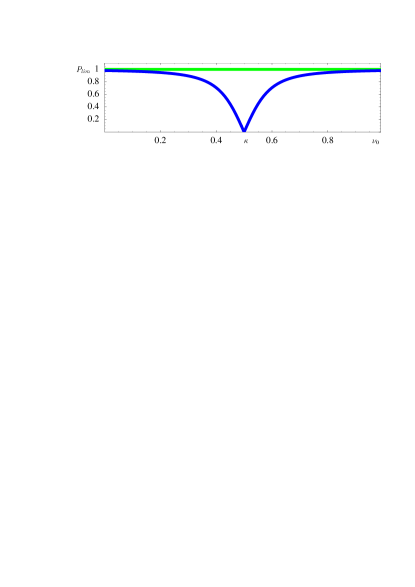
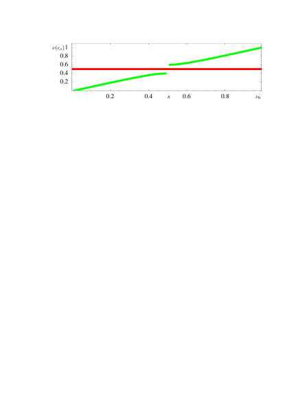
Figure 1: $P_{\mathrm{l}im}$ and the amplitude-dependent spin tune $\nu(\epsilon_{\kappa})$ for the SRM in the vicinity of $\nu_{0}=\kappa$, for $\kappa=0.5$ and $\epsilon_{\kappa}=0.1\;$

Now we want to investigate the crossing of resonances, for the SRM, and describe spin motion when a parameter $\tau$ of the system is being slowly changed, i.e. $\frac{\text{d}}{\text{d}\theta}\tau=\alpha$. In particular this allows the study of an acceleration where $\nu_{0}$ crosses the frequency $\kappa$. It is useful to describe the spin motion in the coordinate system $[\vec{u}_{1},\vec{u}_{2},\vec{n}]$. In order to take account of the change of the basis vectors with the parameter $\tau$, we use that for a vector with $|\vec{u}_{i}|=1$, $\partial_{\tau}\vec{u}_{i}$ is perpendicular to $\vec{u}_{i}$ so that it can be written as a rotation,

$$\frac{\partial}{\partial\tau}\vec{n}=\vec{\eta}\times\vec{n}\ ,\ \ \frac{\partial}{\partial\tau}\vec{u}_{1}=\vec{\eta}\times\vec{u}_{1}\ .$$ (34)

The rotation vector $\vec{\eta}$ is then given by,

$$\vec{\eta}=\frac{1}{2}(\vec{u}_{1}\times\partial_{\tau}\vec{u}_{1}+\vec{u}_{2}\times\partial_{\tau}\vec{u}_{2}+\vec{n}\times\partial_{\tau}\vec{n})\;.$$ (35)

Since $\nu_{0}=G\gamma$ in a flat ring, the acceleration process in the SRM is usually described by a slowly changing $\nu_{0}=\kappa+\tau$ with $\tau=\alpha\theta$ while assuming that $\kappa$ and $\epsilon_{\kappa}$ do not change with energy. This leads to the following expressions for the variation of the basis vectors and for $\vec{\eta}$:

$$\partial_{\tau}\vec{u}_{1} = \mathrm{sig}(\delta)\frac{\epsilon_{\kappa}}{\Lambda^{2}}\vec{n}\cos\Phi\;,$$ (36)

$$\partial_{\tau}\vec{u}_{2} = \mathrm{sig}(\delta)\frac{\epsilon_{\kappa}}{\Lambda^{2}}\vec{n}\sin\Phi\;,$$ (37)

$$\partial_{\tau}\vec{n} = -\mathrm{sig}(\delta)\frac{\epsilon_{\kappa}}{\Lambda^{2}}\vec{\tilde{u}}_{1}\;,$$ (38)

$$\vec{\eta} = \mathrm{sig}(\delta)\frac{\epsilon_{\kappa}}{\Lambda^{2}}\frac{1}{2}(-\vec{\tilde{u}}_{2}-\vec{u}_{2}\cos\Phi+\vec{u}_{1}\sin\Phi)$$ (39)

$$= -\mathrm{sig}(\delta)\frac{\epsilon_{\kappa}}{\Lambda^{2}}\vec{\tilde{u}}_{2}\;.$$

In a general system, the equations of motion for the components of $\vec{S}=\vec{u}_{1}s_{1}+\vec{u}_{2}s_{2}+\vec{n}J_{S}$ are described as

$$\frac{\text{d}}{\text{d}\theta}\left(\begin{array}[]{c}s_{1}\\ s_{2}\\ J_{S}\\ \end{array}\right)=\left(\begin{array}[]{lllll}\alpha(&\eta_{3}s_{2}&-&\eta_{2}J_{S}&)-\nu(\vec{J},\tau)s_{2}\\ \alpha(&\eta_{1}J_{S}&-&\eta_{3}s_{1}&)+\nu(\vec{J},\tau)s_{1}\\ \alpha(&\eta_{2}s_{1}&-&\eta_{1}s_{2}&)\end{array}\right)\;.$$ (40)

In complex notation with $\hat{s}=s_{1}+\text{i}s_{2}$, $\eta=\eta_{1}+\text{i}\eta_{2}$, and $J_{S}=\sqrt{1-|\hat{s}|^{2}}$, this gives

$$\frac{\text{d}}{\text{d}\theta}\hat{s}=i[\nu(\vec{J},\tau)-\alpha\eta_{3}]\hat{s}+\text{i}\alpha\eta\sqrt{1-|\hat{s}|^{2}}\;.$$ (41)

For the SRM, the Eqs. (39) and (30) lead to $\eta=-\text{i}\frac{\epsilon_{\kappa}}{\Lambda^{2}}\text{e}^{\text{i}(\kappa\theta+\Phi_{0})}$, $\eta_{3}=0$, and

$$\frac{\text{d}}{\text{d}\theta}\hat{s}=i[\mathrm{sig}(\delta)\Lambda+\kappa]\hat{s}+\alpha\frac{\epsilon_{\kappa}}{\Lambda^{2}}\text{e}^{\text{i}(\kappa\theta+\Phi_{0})}\sqrt{1-|\hat{s}|^{2}}\;.$$ (42)

Note again that the spin tune $\mathrm{sig}(\delta)\Lambda+\kappa$ in this equation jumps by $2\epsilon_{\kappa}$ at $\nu_{0}=\kappa$.

We will now describe how this equation for the SRM leads to the Froissart-Stora formula. After that, we will use the similarity of the SRM in Eq. (42) and the equation for a general system in Eq. (41) to show how higher-order resonance strength can be introduced and how they can be computed.

III The Froissart-Stora Formula

For the analytically solvable SRM the change of the adiabatic invariant $J_{S}=\vec{S}\cdot\vec{n}$ can be computed explicitly. When the design-orbit spin tune changes during the acceleration process, resonances will be encountered, where $\nu$ jumps from $\kappa\pm\epsilon_{\kappa}$ to $\kappa\mp\epsilon_{\kappa}$ while the spin is under the strong influence of an approximately resonant Fourier contribution of $\omega$. It is then found that for some speeds of the spin tune change, parametrized by $\alpha$, a reduction of polarization can occur is due to a generally irreversible reduction of $J_{S}$ rather than a temporary decrease of $P_{\mathrm{l}im}$, and which does not recover after the energy has increased and the resonance is crossed.

To describe the reduction of polarization during resonance crossing, (42) can be used but the usual approach is to insert a changing closed orbit spin tune $\nu_{0}$ into the equation of motion (13). The method of solution depends on the form of the function $\nu_{0}(\theta)$ froissart60 ; courant80 ; lee97a ; schlesinger85 . If the closed-orbit spin tune changes like $\nu_{0}=\kappa+\alpha\theta$, the equation of spin motion can be solved in terms of confluent hypergeometric functions. The equations for arbitrary initial conditions are quite complicated but when at $\theta\to-\infty$ a vertical spin $s_{3}(-\infty)=1$ is chosen as the initial condition then the vertical component at $\theta\to+\infty$ is given by the well known and regularly used Froissart-Stora formula froissart60 ,

$$s_{3}(\infty)=2\text{e}^{-\pi\frac{\epsilon_{\kappa}^{2}}{2\alpha}}-1\;.$$ (43)

In the case of a strong perturbation $\epsilon_{\kappa}$, or when the acceleration is very slow, spins follow the change of $\vec{n}(\Phi)$. The $\vec{n}$-axis in (15) has a discontinuity from $\vec{n}_{-}=-\epsilon_{\kappa}(\cos\Phi,\sin\Phi,0)^{T}$ just below resonance to $\vec{n}_{+}=-\vec{n}_{-}$ just above resonance. Spins do not follow this instantaneous change of sign, but they then follow $-\vec{n}$ adiabatically after the resonance has been crossed. Therefore $s_{3}(\infty)$ is close to $-1$ for a slow change of $\nu_{0}$. When the perturbation is weak or crossed very quickly, then spin motion is hardly affected and $s_{3}(\infty)$ is close to 1 in (43). In intermediate cases, $|s_{3}|$ is reduced. In the first case the polarization is preserved but the spins are reversed. In the second case the polarization is preserved without reversal. In the third case the polarization is no longer vertical but precesses around the vertical so that the time averaged polarization is reduced.

IV The Froissart-Stora Formula for Higher-Order Resonances

As mentioned above, the Froissart-Stora formula in Eq.(43) is regularly used to describe the reduction of polarization due to vertical betatron motion during resonance crossing in accelerators where the closed-orbit spin tune $\nu_{0}$ changes with energy. These descriptions were normally restricted to flat rings and $\nu_{0}=G\gamma$.

Since Siberian Snakes derbenev76 ; derbenev78a ; derbenev78b ; krisch89a ; luccio94 are unavoidable for high-energy polarized beam acceleration, the design-orbit spin tune is $\frac{1}{2}$ in most cases which will be considered here and it does not change during acceleration. Since the orbital tunes are never chosen to be $\frac{1}{2}$, first-order resonances with $\nu=j_{0}\pm Q_{k}$ are avoided and higher-order resonances can become dominant. But since the strength of such resonances cannot be obtained as a Fourier coefficient of $\omega(\vec{z}(\theta),\theta)$, a method for obtaining the strength of the higher-order resonances is required in order to use the Froissart-Stora formula when Siberian Snakes are in use.

HERA-p will require at least 4 Siberian Snakes hoffstaetter00 ; hoffstaetter02b ; hoffstaetter03 ; hoffstaetter04a . The snake angles $\varphi_{j}$ of these 4 snakes can be chosen quite arbitrarily, except for the restriction $\Delta\varphi=\varphi_{4}-\varphi_{3}+\varphi_{2}-\varphi_{1}=\frac{\pi}{2}$. To illustrate crossing higher-order resonances a snake scheme for HERA-p was chosen that has 4 Siberian Snakes with snake angles of $\frac{\pi}{4}$, $0$, $\frac{\pi}{4}$ and $0$ in the South, East, North and West straight section, respectively.

In Fig. 2 the amplitude-dependent spin tune (green) and $P_{\mathrm{l}im}$ (blue) are plotted versus the reference momentum for a vertical amplitude of $70\pi$ mm mrad. Many higher-order resonances can be observed. The curves for $P_{\mathrm{l}im}$ and $\nu(\vec{J})$ were computed with the non-perturbative algorithm SODOM II yokoya99 using the spin-orbit dynamics program SPRINT man_sprint02 ; hoffstaetter96d . The $\vec{n}$-axis and also $P_{\mathrm{l}im}$ are in general different at different azimuth $\theta_{0}$. For this figure and for all following plots of $P_{\mathrm{l}im}$, the $\vec{n}$-axis was observed at the interaction point of the ZEUS experiment in the South of HERA.

While the design-orbit spin tune remains at $\frac{1}{2}$, the amplitude-dependent spin tune $\nu(J_{y})$ changes with energy and is in resonance with $2Q_{y}$ at the second line (red) and with $5Q_{y}-1$ at the bottom line at several energies. In both cases a clear change of $P_{\mathrm{l}im}$ can be observed. The reduction of $P_{\mathrm{l}im}$ at some resonances is similar to the behavior for the single resonance approximation shown in (33) where $P_{\mathrm{l}im}$ is reduced at those resonances. The drop of $P_{\mathrm{l}im}$ at 811.2 GeV/c is due to the $2-5Q_{y}$ resonance, which lies a little below the $2Q_{y}$ line. At all other energies where this resonance is crossed, no influence on $P_{\mathrm{l}im}$ can be observed since the corresponding fifth-order resonance strength is very small. At some second-order resonances, $P_{\mathrm{l}im}$ increases resonantly. Presumably, two resonant effects are in constructive interference at these energies. Nonetheless, polarization can be reduced when these resonance positions are crossed during acceleration since a sudden increase of $P_{\mathrm{l}im}=$$\langle\vec{n}\rangle$ is due to a sudden change of $\vec{n}(\vec{z})$ which might be too sudden for the adiabatic invariance of $J_{S}=\vec{S}\cdot\vec{n}(\vec{z})$ to be maintained. In addition one can see in Fig. 2 that the spin tune $\nu(J_{y})$ has discontinuities at some of the resonances.

When spin motion in a ring is approximated by a single resonance with $\kappa=j_{0}\pm Q_{y}$ and then Siberian Snakes are included in the ring, it has often been noted that only odd-order resonances with $\kappa=j_{0}+j_{y}Q_{y}$ appear, i.e. $j_{y}$ is odd. However it can be shown by nonlinear normal form theory that this is a feature of any ring with midplane symmetric spin-orbit motion and is not peculiar to rings with Siberian Snakes vogt00 . For rings without midplane symmetry, resonances of even order can appear also. HERA-p has non-flat regions, and rings with closed-orbit distortions in general do not have midplane symmetric motion. Then, resonances with even $j_{y}$ can also appear and be destructive. In fact, the resonances with $j_{y}=2$ are among the most destructive spin-orbit resonances in HERA-p after Siberian Snakes are included. For the IUCF cooler ring with a partial snake running, second-order resonances have been observed experimentally alexeeva95a .

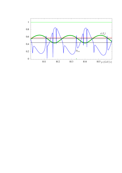
Figure 2: $P_{\mathrm{l}im}$ (blue) and $\nu(J_{y})$ (green) for particles with a $4.2\sigma$ vertical amplitude of $70\pi$ mm mrad in HERA-p with and $Q_{y}=0.289\;$. Three resonance lines cross $\nu$ and at each crossing $P_{\mathrm{l}im}$ exhibits a large variation and there are jumps in $\nu$, bottom: $\nu=5Q_{y}-1$, middle: $\nu=2-5Q_{y}$, and top $\nu=2Q_{y}$

When a parameter $\tau$ is being varied, the spin motion is described in the coordinate system $[\vec{u}_{1},\vec{u}_{2},\vec{n}]$ by Eq. (41). In the following we will demonstrate that this equation has some characteristics of the equation of spin motion (42) of the SRM. If the spin tune $\nu$ has a discontinuity from $\nu_{-}$ to $\nu_{+}$ at some energy, then we define the center frequency $\kappa^{*}=\frac{1}{2}(\nu_{-}+\nu_{+})$. To take the jump of $\nu$ into account, we introduce $\Lambda^{*}=|\nu-\kappa^{*}|$, which does not have a discontinuity and we express the spin tune as $\nu={\rm sig}(\nu-\kappa^{*})\Lambda^{*}+\kappa^{*}$.

Since $\vec{\eta}$ is related to the basis vectors by (35), it is a $2\pi$-periodic function of $\vec{\Phi}$ and $\theta$. The jump of $\nu$ across $\kappa^{*}$ can be produced by a Fourier component of $\eta$ if there is a set of integers so that $\vec{j}\cdot\vec{Q}+j_{0}=\kappa^{*}$. This is the case in all instances of spin tune jumps presented here. Accordingly, one can analyze what happens when the Fourier component $\eta_{\kappa^{*}}\text{e}^{\text{i}(\kappa^{*}\theta+\Phi_{0})}$ of $\eta$ dominates the motion of $\hat{s}$. For that analysis, all other Fourier components of $\eta$ are ignored. When $\alpha$ is small, spins which are initially almost parallel to the $\vec{n}$-axis remain close to $\vec{n}$ so that $\hat{s}$ is small and $\alpha\eta_{3}\hat{s}$ can therefore be ignored. This leads to

$$\frac{\text{d}}{\text{d}\theta}\hat{s}=i(\mathrm{sig}(\nu-\kappa^{*})\Lambda^{*}+\kappa^{*})\hat{s}+I\alpha\eta_{\kappa^{*}}\text{e}^{\text{i}\kappa^{*}\theta+\Phi_{0}}\sqrt{1-|\hat{s}|^{2}}\;.$$ (44)

Due to its similarity with (42), this equation will produce the observed spin tune jump by $2\epsilon_{\kappa^{*}}=|\nu_{+}-\nu_{-}|$ if $\eta_{\kappa^{*}}=\frac{\epsilon_{\kappa^{*}}}{\Lambda^{*2}}=\frac{\epsilon_{\kappa^{*}}}{(\nu-\kappa^{*})^{2}}$ in the vicinity of the energy where the jump occurs. Otherwise (44) would not reproduce this jump. One is then left with a relation which has exactly the structure of the equation of motion (42) for the SRM. Therefore, the Froissart-Stora formula can be applied to estimate how much polarization is lost when a polarized beam is accelerated through the energy region where the spin tune jumps by $2\epsilon_{\kappa}$. In the following we will check whether, for some higher-order resonances in HERA-p, all assumptions leading to the approximation (44) are satisfied to the extent that the Froissart-Stora formula describes the reduction of polarization well.

The basis vectors $\vec{n}$, $\vec{u}_{1}$, and $\vec{u}_{2}$, and the amplitude-dependent spin tune $\nu$ can in general only be computed by computationally intensive methods. The perturbing function $\eta$ is then obtained from

$$\eta = \vec{\eta}\cdot(\vec{u}_{1}+\text{i}\vec{u}_{2})=\vec{\eta}\cdot(-\vec{n}\times\vec{u}_{2}+\text{i}\vec{n}\times\vec{u}_{1})$$ (45)

$$= (\vec{\eta}\times\vec{n})\cdot(-\vec{u}_{2}+\text{i}\vec{u}_{1})=i(\vec{u}_{1}+\text{i}\vec{u}_{2})\cdot(\partial_{\tau}\vec{n})\;,$$

but the required differentiation is prone to numerical inaccuracies. However, when $\vec{n}$ is computed by perturbative normal form theory using differential algebra (DA) balandin92 , the differentiation with respect to $\tau$ can be performed automatically. After $\eta$ is computed, the Fourier integral over the complete ring would finally be required in order to compute $\epsilon_{\kappa}$.

If (41) can be approximated well by a SRM, there is however a different and much less cumbersome method for determining the relevant resonance strength and the resonant frequency. Observation of the amplitude-dependent spin tune $\nu(\vec{J})$ allows the determination of all parameters which are required to evaluate the Froissart-Stora formula for higher-order resonances: The spin tune jumps by $2\epsilon_{\kappa}$, the center of the jump is located at the frequency $\kappa$ itself, and the rate of change of $\nu$ with changing energy is used to determine the parameter $\alpha$ for (43). In the SRM this parameter is $\frac{\nu_{0}-\kappa}{\theta}$ where $\nu_{0}$ is the frequency of spin rotations when the resonance strength vanishes. Here the corresponding frequency, which would be observed if no perturbation $\eta$ were present, is not directly computed. But it can be approximately inferred from the slope $\partial_{\tau}\nu$ at some distance from the resonance.

According to (33), $\langle\vec{n}\rangle$ is given by $P_{\mathrm{l}im}^{SRM}=\sqrt{1-(\frac{\epsilon_{\kappa}}{\nu-\kappa})^{2}}$ in the SRM. To check whether the observed drop of $P_{\mathrm{l}im}$ indeed shows the characteristics of the SRM, the width of the resonance dip in $P_{\mathrm{l}im}^{SRM}$ was obtained from the amplitude-dependent spin tune alone and then compared to the width of the dip in the actual $P_{\mathrm{l}im}$ of the system. This analysis was done for HERA-p’s resonance at approximately 812.4 GeV/c and the results are shown in Fig. 3. The top left plot shows the dependence of $P_{\mathrm{l}im}$ and $\nu$ on the reference momentum for a vertical amplitude of $70\pi$ mm mrad which, with HERA-p’s current one sigma emittance of 4$\pi$ mm mrad, corresponds to the amplitude of a $4.2\sigma$ vertical emittance. The momentum range is as in Fig. 2. The low $P_{\mathrm{l}im}$ shows that many perturbing effects interfere in this region. In units of $\pi$ mm mrad, the vertical amplitude of the particles in the top left graph is 70, in the middle graphs it is 40 and 60, and in the bottom graphs 80 and 100. The horizontal scale displays the distance $\Delta p$ in $GeV/c$ from the momentum at the resonance.

In the 4 bottom graphs, $P_{\mathrm{l}im}$ and $P_{\mathrm{l}im}^{SRM}$ are plotted for different orbital amplitudes, and the different resonance strengths are obtained from the jump in $\nu(J_{y})$. Only information about $\nu$ was used to compute $P_{\mathrm{l}im}^{SRM}$. To allow better comparison, a linear change of $P_{\mathrm{l}im}^{SRM}$ with momentum was added as a background curve and the height of the dip was scaled to fit the actual $P_{\mathrm{l}im}$. The width however was not changed. The distance between spin tune and resonance has been magnified by 10, $\nu^{*}=\kappa+10(\kappa-\nu)$ in these graphs. The tune jump is symmetric around the resonance line $\nu=2Q_{y}$, showing that a second-order resonance is excited.

As shown in Fig. 3 (top right) the tune jump scales approximately linearly with the orbital action variable $J_{y}$. This is consistent with the crossing of a second-order resonance, since a frequency of $2Q_{y}$ can be produced by monomials of $\sqrt{J_{y}}\text{e}^{\pm\text{i}Q_{y}\theta}$ with order larger or equal to 2. This linear scaling is not exact for two reasons: (1) The jump does not reduce to 0 at $J_{y}=0$ but already at some finite amplitude at which $\nu(J_{y})$ does not cross the resonance line. (2) When the amplitude is changed, the momentum at which the resonance occurs changes, and the resonance strength is in general different at different energies. Deviations from a linear dependence should therefore be expected. $P_{\mathrm{l}im}$ is already very low away from the resonance at $\nu=2Q_{y}$, indicating that other strong perturbations distort the invariant spin field and can interfere with the resonance harmonic.

Thus we conclude that the resonance width computed in terms of the tune jump $2\epsilon_{\kappa}$ agrees surprisingly well with the actual drop in $P_{\mathrm{l}im}$.

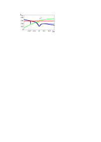
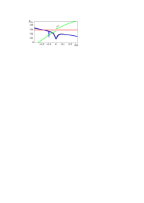
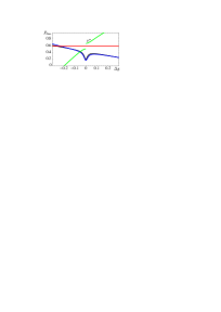
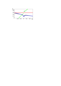
Figure 3: Top left: $P_{\mathrm{l}im}$ and $\nu$ in the vicinity of the resonance at approximately 812.4 GeV/c for HERA-p. The distance between $\nu$ and resonance has been magnified by 10, $\nu^{*}=\kappa+10(\kappa-\nu)$. Top right: Proportionality between tune jump $2\epsilon_{k}$ and the amplitude $2J_{y}$ of a vertical emittance. Middle and bottom: Correlation between the width of the actual drop of $P_{\mathrm{l}im}$ and the predictions of the single resonance approximation using only the amplitude-dependent spin tune. Vertical amplitudes of particles in HERA-p in units of $\pi$ mm mrad from top left to bottom right: 70, 40, 60. 80, and 100. $\Delta p$: distance from the momentum at resonance in GeV/c

Since the higher-order resonances analyzed here show the established and characteristic relation between tune jump and reduction of $P_{\mathrm{l}im}$, the applicability of the Froissart-Stora formula will now be tested.

In Fig. 4 (top) $P_{\mathrm{l}im}$ and $\nu$ are shown for HERA-p. $P_{\mathrm{l}im}$ is reduced at two resonances with $\nu=2Q_{y}$. The vertical tune had been chosen as $Q_{y}=0.2725$ so that these resonances are crossed already for the small $0.75\sigma$ vertical amplitude of $2.25\pi$ mm mrad. At this small amplitude $P_{\mathrm{l}im}$ is reasonably large.

The spins of a set of particles were set parallel to the invariant spin field $\vec{n}(\vec{z})$ so that all had $J_{S}=1$ at the momentum of 801 GeV/c. The $\vec{n}$-axis had been computed by stroboscopic averaging hoffstaetter96d . Due to the rather large $P_{\mathrm{l}im}$ at that energy the initial polarization was approximately 97%. Starting with this spin configuration, the beam was accelerated to 804 GeV/c at various rates. The average $\langle J_{S}\rangle_{N}$ over the tracked particles is plotted versus acceleration rate in Fig. 4 (bottom) together with the prediction of the Froissart-Stora formula. The average $\langle J_{S}\rangle_{N}$ describes the degree of beam polarization which could be recovered due to the adiabatic invariance of $J_{S}$ when moving into an energy regime where $\vec{n}(\vec{z})$ is close to parallel to the vertical.

The resonance strength $\epsilon_{2Q_{y}}$ has been determined from the tune jump. The parameter $\alpha$ is proportional to the energy increase per turn $d_{E}$ and is determined from the tune slope $\frac{\Delta\nu}{\Delta E}$ in Fig. 4 (top right) by the relation $\alpha=\frac{1}{2\pi}\frac{\Delta\nu}{\Delta E}d_{E}$.

The polarization obtained by accelerating particles through the second-order resonance agrees remarkably well with the Froissart-Stora formula. For the slow acceleration of about $50$ keV per turn in HERA-p, the polarization would be completely reversed on the $0.75$ sigma invariant torus. This would lead to a net reduction of beam polarization, since the spins in the center of the beam are not reversed.

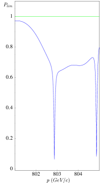
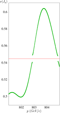
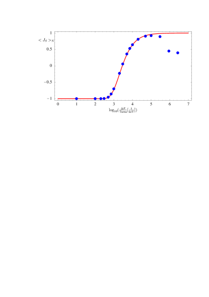
Figure 4: Top: $P_{\mathrm{l}im}$ and $\nu$ for a second-order resonance of HERA-p with $Q_{y}=0.2725$ and a $0.75\sigma$ vertical amplitude of $2.25\pi$ mm mrad. Bottom: $\langle J_{S}\rangle_{N}$ after acceleration from 801 GeV/c to 804 GeV/c with different acceleration rates (blue points) and the prediction of the Froissart-Stora formula (red curve) using parameters $\epsilon_{2Q_{y}}$ and $\alpha$ obtained from $\nu$

This result on the applicability of (43) for the resonance strength and $\alpha$ obtained from the amplitude dependent spin tune is so important for detailed analysis of the acceleration process that it will be checked in another case. In the next example, the same lattice is used, the tune was adjusted to a realistic value of $Q_{y}=0.289$ and a $4.2\sigma$ vertical amplitude of $70\pi$ mm mrad was chosen. At this large amplitude, the second and fifth-order resonances already shown in Fig. 2 are observed. Particles were then accelerated from 812.2 GeV/c to 812.6 GeV/c with different acceleration rates. Note that the initial condition has a vertical polarization of only 60%. Nevertheless this state of polarization corresponds to a completely polarized beam, and 100% polarization can potentially be recovered by changing the energy adiabatically into a region where $\vec{n}(\vec{z})$ is tightly bundled. These studies emphasize again the importance of choosing $\vec{n}(\vec{z})$ as the initial spin direction. For example if the spins were initially polarized vertically, they would rotate around $\vec{n}(\vec{z})$ and that would lead to a fluctuating polarization, even without a resonance and it would not be possible to establish a Froissart-Stora formula for higher-order resonances.

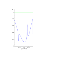
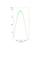
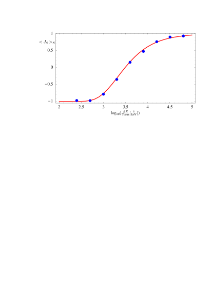
Figure 5: Top: $P_{\mathrm{l}im}$ and $\nu$ for a second-order resonance of HERA-p with realistic tune of $Q_{y}=0.289$ and a large $4.2\sigma$ vertical amplitude of $70\pi$ mm mrad. Bottom: $\langle J_{S}\rangle_{N}$ after acceleration from 812.2 GeV/c to 812.6 GeV/c with different acceleration rates (blue points) and the prediction of the Froissart-Stora formula (red curve) using parameters $\epsilon_{2Q_{y}}$ and $\alpha$ obtained from $\nu$

As shown in Fig. 5, $P_{\mathrm{l}im}$ is as low as 0.11 in the center of the displayed region. Obviously other strong effects beyond the second-order resonance are present and overlap with it. The bottom figure shows $\langle J_{S}\rangle_{N}$ after the acceleration. The fact that $\langle J_{S}\rangle_{N}$ is again described very well by the Froissart-Stora formula (43) is an impressive confirmation of the conjecture.

The two data points at largest acceleration speed in Fig. 4 (bottom) are lower than predicted by the Froissart-Stora formula. A possible explanation is the following: at very large acceleration speeds the resonance region is crossed so quickly that the spin motion is hardly disturbed. But when the $\vec{n}$-axis $\vec{n}_{-}$ before the resonance region is not parallel to the $\vec{n}$-axis $\vec{n}_{+}$ after the resonance region, then the spins which initially had $J_{S}=1$ will approximately have $J_{S}=\vec{n}_{-}\cdot\vec{n}_{+}$ after the resonance region is crossed, which is smaller than the Froissart-Stora prediction, which approaches 1 for large acceleration speeds.

Here the parameter $\tau$ was the slowly changing momentum. This generalized way of using the Froissart-Stora formula can however also be used when other system parameters change. An example can be found in hoffstaetter98d , where the particle’s phase space amplitude is changed artificially slowly in order to compute the invariant spin field at various orbital amplitudes. In vogt00 an example is displayed where the Froissart-Stora formula is successfully applied to a resonance which is encountered because of a slow variation of $Q_{y}$.

V The Choice of Orbital Tunes

When the amplitude-dependent spin tune $\nu(\vec{J})$ of particles with the amplitude $\vec{J}$ crosses a resonance, for example during acceleration, the beam polarization is usually reduced.

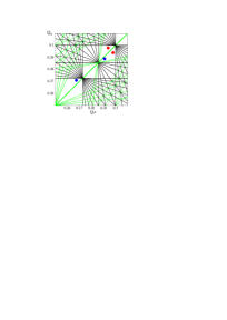
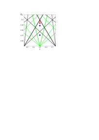
Figure 6: Left: the current orbit tunes ($Q_{x}=0.294$,$Q_{y}=0.298$) or ($Q_{x}=0.298$,$Q_{y}=0.294$) (red) and the new orbit tunes for polarized proton operation ($Q_{x}=0.291$,$Q_{y}=0.289$) or ($Q_{x}=0.2675$, $Q_{y}=0.271$) (blue) in the $x$-$y$ resonance diagram. All resonances up to order 11 are shown. Difference resonances are indicated in green. Right: The current vertical tunes (red) and the new vertical tunes (blue) in the spin-orbit resonance diagram. The odd spin-orbit resonances (black) and the even spin-orbit resonances (green) are shown up to order 10 in the vicinity of closed-orbit spin tune $\nu_{0}=\frac{1}{2}$. For HERA-p, the resonances of second order (fat green) and of fifth order (fat black) are most destructive

It is therefore important to find suitable orbital tunes so that low-order spin-orbit resonances are far away from the operating point. In particular, when Siberian Snakes are used to maintain a closed orbit spin tune of $\frac{1}{2}$, it is important that these Snakes are optimized so that higher-order resonances do not lead to large deviations of the amplitude dependent spin tune from this value. Such optimal choices of snakes are discussed in hoffstaetter04a . The dominant effects are due to radial fields on vertical betatron trajectories. Thus Fig. 6 (right) shows the resonance lines $\nu=j_{0}+jQ_{y}$ up to order 10 in the $\nu$-$Q_{y}$ plane. If the spin tune on the closed orbit is fixed to $\nu_{0}=\frac{1}{2}$ by Siberian Snakes the orbital tune can be chosen to avoid resonance lines. However, the dynamic aperture of proton motion should not be reduced and the tunes have to be far away from low order orbital resonances. Figure (6) (left) shows the $Q_{x}$-$Q_{y}$ tune diagram with resonance lines up to order 11. The operating point has to stay away from these resonance lines.

The established tunes of HERA-p operation $Q_{x}=0.294$, $Q_{y}=0.298$ or $Q_{x}=0.298$, $Q_{y}=0.294$ (red points) would be unfortunate choices due to their closeness to the resonance $\nu=j_{0}\pm 5Q_{y}$. For HERA-p with Siberian Snakes, several simulations have shown that the resonances of second order and of fifth order are most destructive. This is supported by Fig. 2. Therefore two new tunes (blue points) are suggested which have an optimal distance from low-order spin-orbit resonances. It has been tested experimentally that HERA-p could operate at these tunes.

References

- (1) E. D. Courant and R. D. Ruth: The acceleration of polarized protons in circular accelerators. BNL–51270 and UC–28 and ISA–80–5 (1980)
- (2) G.H. Hoffstaetter: Polarized protons in HERA. In Proceedings of NUCLEON99, Nucl. Phys. A (1999)
- (3) Ya. S. Derbenev and A. M. Kondratenko: Diffusion of particle spin in storage rings. Sov. Phys. JETP, 35:230 (1972)
- (4) K. Yokoya: The action–angle variables of classical spin motion in circular accelerators. DESY–86–057 (1986)
- (5) L. H. Thomas: The kinematics of an electron with an axis. Phil. Mag. 3(13):1–20 (1927)
- (6) V. Bargmann, L. Michel, and V. L. Telegdi: Precession of the polarization of particles moving in a homogeneous electro–magnetic field. Phys. Rev. Lett. 2(10):435–436 (1959)
- (7) G.H. Hoffstaetter: Aspects of the Invariant Spin Field for High Energy Polarized Proton Beams. Habilitation, Darmstadt University of Technology, (January 2000)
- (8) G. H. Hoffstaetter, H. S. Dumas and J. A. Ellison: Adiabatic invariants for spin-orbit motion. In Proceedings to EPAC02, Paris and DESY-M-02–01 (2002)
- (9) A. I. Neistadt: Passage through resonance in a two-frequency problem. Soviet Phys. Doklady, 20(3):189–191, 1975. English translation of Doklady Akad. Nauk. SSSR Mechanics 221 (2), 301–304 (1975)
- (10) M. Vogt: Bounds on the maximum attainable equilibrium spin polarization of protons in HERA. Dissertation, Universität Hamburg, DESY-THESIS-2000-054 (December 2000)
- (11) D. P. Barber, J. A. Ellison, K. Heinemann: Phys. Rev. ST-AB, submitted (2004)
- (12) A. I. Neistadt: Averaging in multi-frequency systems. Soviet Phys. Doklady, 20(7):492–494, 1976. English translation of Doklady Akad. Nauk. SSSR Mechanics 223 (2), 314–317 (1976)
- (13) K. Abragam: The principles of nuclear magnetism. Clarendon (1961)
- (14) S. R. Mane: Exact solution of the Derbenev–Kondratenko –axis for a model with one resonance. FERMILAB–TM–1515 (1988)
- (15) K. Heinemann and G. H. Hoffstaetter: A tracking algorithm for the stable spin polarization field in storage rings using stroboscopic averaging. Phys. Rev. E 54:4240–4255 (1996)
- (16) M. Froissart and R. Stora: Depolarisation d’un faisceau de protons polarises dans un synchrotron. Nucl. Instr. Meth. 7:297–305 (1960)
- (17) M. F. Schlesinger: The wonderful world of stochastics. Studies in statistical mechanics 12. North-Holland, p. 382 (1985)
- (18) S. R. Mane: Electron-spin polarization in high–energy storage rings. II. Evaluation of the equilibrium polarization. Phys. Rev. A(36):120–130 (1987)
- (19) S. Y. Lee and S. Tepikian: Resonance due to a local spin rotator in high–energy accelerators. Phys. Rev. Lett. 56(16):1635–1638 (1986)
- (20) S. Y Lee: Spin–depolarization mechanisms due to overlapping spin resonances in synchrotrons. Phys. Rev. E 47(5):3631–3644 (1993)
- (21) S. Y. Lee: Spin dynamics and Snakes in synchrotrons. World Scientific (1997)
- (22) Ya. S. Derbenev and A. M. Kondratenko: Acceleration of polarized particles. Sov. Phys. Doklady, 20:562, 1976. also in russ.: Dokl.Akad.Nauk Ser.Fiz.223:830-833 (1975)
- (23) Ya. S. Derbenev, A. M. Kondratenko, S. I. Serednyakov, et al: Radiative polarization: obtaining, control, using. Particle Accelerators, 8:115–126 (1978)
- (24) Ya. S. Derbenev and A. M. Kondratenko: On the possibilities to obtain high-energy polarized particles in accelerators and storage rings. In G. H. Thomas, editor, High–energy Physics with Polarized Beams and Polarized Targets, AIP Conference Proceedings 51, p. 292 (1978)
- (25) A. D. Krisch, S. R. Mane, R. S. Raymond, T. Roser, et al: First test of the Siberian Snake magnet arrangement to overcome depolarizing resonances in a circular accelerator. Phys. Rev. Lett. 63(11):1137–1140 (1989)
- (26) A. Luccio and T. Roser, editors: Third workshop on Siberian Snakes and spin rotators. BNL–52453, Brookhaven (1994)
- (27) D. P. Barber, G. H. Hoffstaetter and M. Vogt: Polarized protons in HERA. In Proceedings to EPAC02, Paris and DESY-M-02–01 (2002)
- (28) G.H. Hoffstaetter: Matching of Siberian Snakes. AIP Conf.Proc.667:93-102 (2003)
- (29) G.H. Hoffstaetter: Optimal Axes of Siberian Snakes for Polarized Proton Acceleration submitted to Phys. Rev. ST-AB (2004)
- (30) G. H. Hoffstaetter, Future possibilities for HERA, In Proceedings EPAC00, Vienna (2000)
- (31) K. Yokoya: An algorithm for calculating the spin tune in circular accelerators. DESY-99-006 (1999)
- (32) G. H. Hoffstaetter and M. Vogt: Sprint users guide and reference manual. DESY (2002)
- (33) C. Ohmori, H. Sato, L. V. Alexeeva, V. A. Anferov, D. D. Caussyn, C. M. Chu, D. A. Crandell, S. E. Gladycheva, S-Q. Hu, A. D. Krisch, R. A. Phelps, S. M. Varzar, and V. K. Wong, S. Y. Lee, T. Rinckel, P. Schwandt, F. Sperisen, E. J. Stephenson, and B. von Przewoski, R. Baiod and A. D. Russell: Observation of a second–order spin–depolarizing resonance. Phys. Rev. Lett. 75(10):1931–1933 (1995)
- (34) V. Balandin and N. Golubeva: Nonlinear spin dynamics. Proceedings of the XV International Conference on High–energy Particle Accelerators, Hamburg, p. 998–1000 (1992)
- (35) D. P. Barber, M. Vogt, and G. H. Hoffstaetter: The amplitude–dependent spin tune and the invariant spin field in high–energy proton accelerators. In Proceedings EPAC98, Stockholm (1998)