Beam-Breakup Instability Theory for Energy Recovery Linacs

Abstract

Here we will derive the general theory of the beam-breakup instability in recirculating linear accelerators, in which the bunches do not have to be at the same RF phase during each recirculation turn. This is important for the description of energy recovery linacs (ERLs) where bunches are recirculated at a decelerating phase of the RF wave and for other recirculator arrangements where different RF phases are of an advantage. Furthermore it can be used for the analysis of phase errors of recirculated bunches. It is shown how the threshold current for a given linac can be computed and a remarkable agreement with tracking data is demonstrated. The general formulas are then analyzed for several analytically solvable cases, which show: (a) Why different higher order modes (HOM) in one cavity do not couple so that the most dangerous modes can be considered individually. (b) How different HOM frequencies have to be in order to consider them separately. (c) That no optics can cause the HOMs of two cavities to cancel. (d) How an optics can avoid the addition of the instabilities of two cavities. (e) How a HOM in a multiple-turn recirculator interferes with itself. Furthermore, a simple method to compute the orbit deviations produced by cavity misalignments has also been introduced. It is shown that the BBU instability always occurs before the orbit excursion becomes very large.

I Introduction

Synchrotron light sources based on Energy Recovery Linacs (ERLs) show promise to deliver X-ray beams with both brilliance and X-ray pulse duration far superior to the values that can be achieved with storage ring technology. This is due to the fact that the emittances in an ERL are largely determined by a laser-driven source, technology which has been improving steadily over the years, and will undoubtedly improve further. To generate high brilliance high flux X-rays it is necessary to accelerate beams to the energies (several GeV) and with the currents (several $100$ mA) that are typical in these storage rings. This would require that the linac delivers a power of order $1$ GW to the beam. Without somehow recovering this energy after the beam has been used, such a device would be practically unfeasible. Energy recovery Tigner65_01 can be achieved by decelerating high energy electrons to generate cavity fields which in turn accelerate new electrons to high energy. With this, large beam powers that are not accessible in a conventional linac, can be produced.

Several laboratories have proposed high power ERLs for different purposes. Designs for light production with different parameter sets and various applications are being worked on by Cornell University CHESS01_03 ; ERL03_12 , BNL Benzvi01_02 , Daresbury Pool03_01 , TJNAF Benson01_01 , JAERI Sawamura03_02 , the University of Erlangen Berkaev02_01 , Novosibirsk Kulipanov98_01 , and KEK Suwada02_01 . TJNAF has incorporated an ERL in its design of an electron–ion collider (EIC) Merminga02_01 for medium energy physics, while BNL is working on an ERL–based electron cooler Benzvi03_01 for the ions in the relativistic ion collider (RHIC). The work at TJNAF, JAERI and Novosibirsk is based on existing ERLs of relatively small scale.

One important limitation to the current that can be accelerated in such an ERL is given by the beam-breakup (BBU) instability. The size and cost of all these new accelerators certainly requires a very detailed understanding of this limitation.

A theory of BBU instability in recirculating linacs, where the energy is not recovered in the linac, but where energy is added to the beam when it returns after each recirculation turn, was presented in Bisognano87_01 . Such a linac can consists of many cavities and several recirculation turns can be used. This original theory was additionally restricted to scenarios where the bunches of the different turns are in the linac at about the same accelerating RF phase, such as in the so-called continuous wave (CW) operation where every bucket is filled. Tracking simulations Krafft87_01 compared well with this theory. In the following we therefore refer to it as the CW recirculator BBU theory. It determines above what threshold current $I_{\rm th}$ the transverse bunch position $x$ displays undamped oscillations in the presence of a higher order mode (HOM) with frequency $\omega_{\lambda}$. If there is only one higher order mode and one recirculation turn with a recirculation time $t_{r}$ in the linac, the following formula is obtained for $T_{12}\sin\omega_{\lambda}t_{r}<0$:

$$I_{\rm th}=-\frac{2c^{2}}{e(\frac{R}{Q})_{\lambda}Q_{\lambda}\omega_{\lambda}}\frac{1}{T_{12}\sin\omega_{\lambda}t_{r}}\ ,$$ (1)

where $c$ is the speed of light, $T_{12}$ is the element of the transport matrix that relates initial transverse momentum $p_{x}$ before and $x$ after the recirculation loop, $e$ is the elementary charge, $(R/Q)_{\lambda}Q_{\lambda}$ is the impedance (in units of $\Omega$) of the higher order mode driving the instability, $Q_{\lambda}$ is its quality factor. A corresponding formula had already been presented in randbook . Occasionally, additional factors are found when this equation is stated Sereno94 ; Beard03_01 ; Merminga01_01 . We give a concise derivation which shows that no such additional factors are required.

In the past efforts have been made to derive threshold currents from the analysis of experimental data obtained at the TJNAF FEL-ERL Sereno94 ; Merminga01_01 using the CW recirculator BBU theory. The data has not been interpreted satisfactorily, and at least part of the reason could be that the underlying theory had not been derived for ERL operation. The theory presented in this paper should therefore be used to extend and improve these previous analysis results, as it is directly applicable to ERL operation.

Here we will derive the general theory of the beam-breakup instability in recirculating linear accelerators, in which the bunches do not have to be at the same RF phase during each recirculation turn, similar to what has first been presented in Yunn91_01 . First we treat the simplest case of one dipole HOM and one recirculation turn. Then we allow many HOMs and many recirculations, and finally we analyze several analytically solvable cases.

II One Dipole HOM and One Recirculation

For recirculating linacs, the simplest case of one HOM and one recirculation loop has long been described Bisognano86_01 . Previous theories which assume that the recirculation time is an integral number of RF periods should not be used when investigating ERLs. Next we derive more general formulas that may be applied for arbitrary recirculation times.

II.1 The Dispersion Relation

In the simplest model of multi-pass beam breakup, bunches are injected into a cavity, which is assumed to have one dipole HOM (e.g. $TM_{11}$-like mode), accelerated in the cavity and then recirculated to pass the cavity a second time before they are ejected. In the case of a two-turn recirculating linac, each bunch would be accelerated on both passes through the linac and ejected to a user area. The RF phase of the bunch would therefore be approximately the same on both passes. In an ERL, the RF phase on the second pass through the cavity is shifted by $\pi$ with respect to the first pass so that the energy that the bunch gains in the first pass is returned to the cavity during the second pass and the bunch is ejected with reduced energy into a beam dump.

If a dipole HOM is excited in the cavity, then a bunch that enters the cavity on axis experiences a transverse kick and starts to oscillate around the design orbit of the recirculation loop and returns to the cavity with a transverse offset. This offset leads to a change in the energy of the HOM. If it increases the HOM energy, transverse kicks experienced by subsequent bunches will be larger, which will in turn lead to a further growth of the HOM energy once the kicked bunch returns to the linac: an instability develops.

To describe this effect, we use the ideas and nomenclature from krafft89 . When a current $I(t^{\prime})$ passes the cavity during its recovery loop at a time $t^{\prime}$, the charge $I(t^{\prime})dt^{\prime}$ with the transverse offset $x(t^{\prime})$ excites the dipole HOM, creating a transverse momentum for particles traveling through the cavity subsequently at time $t$,

$$\Delta p_{x}(t)=\frac{e}{c}W(t-t^{\prime})x(t^{\prime})I(t^{\prime})dt^{\prime}\ ,$$ (2)

where the wake function $W(\tau)$ describes the transverse force at time $\tau$ after the HOM was excited. The momentum transfer is described by an effective transverse voltage of the HOM, $V(t)=\frac{c}{e}\Delta p_{x}(t)$.

Assuming that all bunches are injected on the cavity’s central axis, they do not excite dipole HOMs on their first path through the cavity. However, the effective transverse voltage of the HOM determines what kick $\Delta p_{x}(t)$ the bunch sees and what position it will have when it returns to the cavity after the recirculation time $t_{r}$. The transfer matrix element $T_{12}$ maps the transverse momentum $p_{x}(t)$ to $x(t+t_{r})=T_{12}p_{x}(t)$. Inserting this into Eq. (2) leads to an integral equation for the HOM’s effective voltage,

$$V(t)=\int_{-\infty}^{t}W(t-t^{\prime})I(t^{\prime})T_{12}\frac{e}{c}V(t^{\prime}-t_{r})dt^{\prime}\ .$$ (3)

To solve this integral equation, one assumes that the current is a continuous stream of short pulses being injected at multiples of an interval between bunches $t_{b}$, so that the current on the second turn is given by

$$I(t)=I_{0}t_{b}\sum_{m=-\infty}^{\infty}\delta_{D}(t-t_{r}-mt_{b})\ ,$$ (4)

$\delta_{D}$ being the Dirac-delta function. Note that $t_{b}$ is an integer multiple of the RF circulation time $t_{0}=2\pi/\omega_{0}$ for the RF frequency $\omega_{0}$. We write the recirculation time in terms of the time $t_{b}$ between bunches as

$$t_{r}=(n_{r}-\delta)t_{b}\ ,$$ (5)

with an integer $n_{r}$ and $\delta\in[0,1)$. For a recirculating linac one has

$$\delta t_{b}\approx nt_{0}\ ,$$ (6)

and for an ERL one has $\delta t_{b}\approx(n+\frac{1}{2})t_{0}$ for some integer $n$. A “$+$” sign in Eq. 5 that defines $\delta$ may seem more natural but our choice leads to simplified equations.

The HOM voltage at a time $t\in[nt_{b}+t_{r},nt_{b}+t_{r}+t_{b})$ is given by

$$V(t)=I_{0}t_{b}T_{12}\frac{e}{c}\sum_{m=-\infty}^{n}W(t-t_{r}-mt_{b})V(mt_{b})\ .$$ (7)

Evaluating this at the time $t=nt_{b}+t_{r}$ when the recirculated bunches pass through the cavity leads to

$$V(nt_{b}+t_{r})=I_{0}t_{b}T_{12}\frac{e}{c}\sum_{m=0}^{\infty}W(mt_{b})V([n-m]t_{b})\ .$$ (8)

In the CW recirculator BBU theory this difference equation was dealt with by assuming that the voltage can be written as $V(t)=V_{0}e^{-i\omega t}$ for $t=nt_{b}$ where a positive imaginary part of $\omega$ indicates instability. Note that this does not require $V(t)$ to be a harmonic function, but that it can be a linear combination of harmonic functions with frequencies $\omega+m\frac{2\pi}{t_{b}}$ for integers $m$. This distinction has not been always made clear and is a potential source of confusion Sereno94 . One obtains the equation

$$\frac{1}{I_{0}}=t_{b}T_{12}\frac{e}{c}e^{i\omega t_{r}}\sum_{m=0}^{\infty}W(mt_{b})e^{i\omega mt_{b}}\ .$$ (9)

The smallest value of the current $I_{0}$ for which there is a real $\omega$ is the threshold current $I_{\rm th}$ of the instability.

We proceed by writing $V(t)$ in terms of its Laplace transform, retaining all possible frequencies in HOM voltage, which automatically enables proper description of arbitrary recirculating configuration:

$$V(t)=\frac{1}{2\pi}\int_{-\infty-ic_{0}}^{\infty-ic_{0}}\tilde{V}(\omega^{\prime})e^{-i\omega^{\prime}t}d\omega^{\prime}\ .$$ (10)

Note that this is not the conventional way of writing a Laplace transform. We have chosen this notation in order to make it appear more similar to a Fourier Transform. It also makes the subsequent notation more similar to the CW recirculator BBU theory. The Laplace transform is used rather than the Fourier transform since we want to analyze the onset of instability where the frequencies $\omega$ become complex. With the following definition

$$\tilde{V}^{\Sigma}(\omega)=\sum_{n=-\infty}^{\infty}\tilde{V}(\omega+\frac{2\pi}{t_{b}}n)$$ (11)

we obtain

$$\tilde{V}^{\Sigma}(\omega)=t_{b}\sum_{n=-\infty}^{\infty}V(nt_{b})e^{i\omega nt_{b}}\ .$$ (12)

Since $\tilde{V}^{\Sigma}(\omega)$ is periodic with $2\pi/t_{b}$, it has a Fourier series, and its Fourier coefficients are $V(nt_{b})$. This shows that $\tilde{V}^{\Sigma}(\omega)$ does not vanish. We can therefore choose $t=(n+n_{r})t_{b}$ in Eq. (7) and sum over $n$,

$$\tilde{V}^{\Sigma}(\omega)=t_{b}\sum_{n=-\infty}^{\infty}V([n+n_{r}]t_{b})e^{i\omega[n+n_{r}]t_{b}}$$

$$= I_{0}t_{b}^{2}T_{12}\frac{e}{c}$$

$$\times \sum_{n=-\infty}^{\infty}\sum_{m=0}^{\infty}W([m+\delta]t_{b})V([n-m]t_{b})e^{i\omega[n+n_{r}]t_{b}}$$

$$= I_{0}t_{b}T_{12}\frac{e}{c}e^{i\omega n_{r}t_{b}}\sum_{m=0}^{\infty}W([m+\delta]t_{b})e^{i\omega mt_{b}}\tilde{V}^{\Sigma}(\omega)\ .$$

This finally yields the dispersion relation between $I_{0}$ and $\omega$ which can be used for all $\delta$. A corresponding derivation, which has treated the beam recirculation in a way that can be applied to ERLs, has been presented in Yunn91_01 . We believe that this paper should be referenced more often, since it is hardly referenced, whereas the earlier papers with CW recirculator BBU theory, which was not derived for ERLs, are often referenced in the context of ERLs, where they are not strictly applicable.

II.2 The Far-Field Wake

The sum in the dispersion relation

$$\frac{1}{I_{0}} = t_{b}T_{12}\frac{e}{c}e^{i\omega n_{r}t_{b}}w(\delta)\ ,$$ (14)

$$w(\delta) = \sum_{n=0}^{\infty}W([n+\delta]t_{b})e^{i\omega nt_{b}}\ ,$$ (15)

can be computed when the far-field approximation for the wake function is used,

$$W(\tau)=\left(\frac{R}{Q}\right)_{\lambda}\frac{\omega_{\lambda}^{2}}{2c}e^{-\frac{\omega_{\lambda}}{2Q_{\lambda}}\tau}\sin\omega_{\lambda}\tau\ .$$ (16)

With $\omega_{\lambda}^{\pm}=\omega_{\lambda}\pm i\frac{\omega_{\lambda}}{2Q_{\lambda}}$ and $\omega^{+}=\omega+i\frac{\omega_{\lambda}}{2Q_{\lambda}}$ the required sum can be evaluated if ${\rm Im}(\omega)>-\frac{\omega_{\lambda}}{2Q_{\lambda}}$ and becomes

$$w(\delta) = \sum_{n=0}^{\infty}W([n+\delta]t_{b})e^{i\omega nt_{b}}$$

$$= \left(\frac{R}{Q}\right)_{\lambda}\frac{\omega_{\lambda}^{2}}{4ic}\left[\frac{e^{i\omega_{\lambda}^{+}\delta t_{b}}}{1-e^{i(\omega_{\lambda}^{+}+\omega)t_{b}}}-\frac{e^{-i\omega_{\lambda}^{-}\delta t_{b}}}{1-e^{-i(\omega_{\lambda}^{-}-\omega)t_{b}}}\right]$$

$$= \left(\frac{R}{Q}\right)_{\lambda}\frac{\omega_{\lambda}^{2}}{4c}e^{-i\omega\delta t_{b}}$$

$$\times \frac{e^{i\omega^{+}(\delta-1)t_{b}}\sin(\omega_{\lambda}\delta t_{b})-e^{i\delta\omega^{+}t_{b}}\sin(\omega_{\lambda}[\delta-1]t_{b})}{\cos\omega^{+}t_{b}-\cos\omega_{\lambda}t_{b}}\ .$$

The dispersion relation thus becomes

$$I_{0}=\frac{2}{\mathcal{K}T_{12}}e^{-i\omega n_{r}t_{b}}\frac{e^{\frac{\omega_{\lambda}}{2Q_{\lambda}}\delta t_{b}}[\cos(\omega^{+}t_{b})-\cos(\omega_{\lambda}t_{b})]}{e^{-i\omega^{+}t_{b}}\sin(\delta\omega_{\lambda}t_{b})-\sin([\delta-1]\omega_{\lambda}t_{b})}\ ,$$ (18)

with $\mathcal{K}=t_{b}\frac{e}{c^{2}}(\frac{R}{Q})_{\lambda}\frac{\omega_{\lambda}^{2}}{2}$. For $\delta=0$ this becomes the dispersion relation of the CW recirculator BBU theory:

$$I_{0}=\frac{2}{\mathcal{K}T_{12}}e^{-i\omega t_{r}}\frac{\cos(\omega^{+}t_{b})-\cos(\omega_{\lambda}t_{b})}{\sin(\omega_{\lambda}t_{b})}\ .$$ (19)

This describes the case when the recirculated bunches are in the same buckets as the accelerated bunches. When the recirculated bunches are just between accelerated bunches, then $\delta=\frac{1}{2}$,

$$I_{0}=\frac{1}{\mathcal{K}T_{12}}e^{-i\omega t_{r}}\frac{\cos(\omega^{+}t_{b})-\cos(\omega_{\lambda}t_{b})}{\cos(\omega^{+}t_{b}/2)\sin(\omega_{\lambda}t_{b}/2)}\ .$$ (20)

For the case that every bucket is filled, this would be an ERL with $t_{b}=t_{0}$. The dispersion relation for ERLs for other $\delta$ is less simple than Eq. (20) and has $\delta t_{b}=(n+\frac{1}{2})t_{0}$ in Eq. (18). This occurs when the decelerating and accelerating bunches are not perfectly centered between each other.

II.3 The Threshold Current

For a given positive current $I_{0}$, the values of $\omega$ that satisfy the dispersion relation Eq. (18) will in general be complex. If they all have negative imaginary parts, the beam motion is stable. If one of them has positive imaginary part it will be unstable.

For small currents the beam motion is stable. When the current is increased, at some point, one of these $\omega$ will become real. At this point the threshold current is reached. The threshold current $I_{\rm th}$ is therefore the smallest current $I_{0}$ for which there is a real $\omega$ that satisfies the dispersion relation. To find this current, we note that

$$I_{0}(\omega+\frac{2\pi}{t_{b}})=I_{0}(\omega)\ ,\ \ I_{0}(-\omega^{*})=I_{0}^{*}(\omega)\ .$$ (21)

It is therefore sufficient to investigate $\omega\in[0,\pi/t_{b}]$.

Figure 1 shows $I_{0}(\omega)$ in the complex plain for $\omega\in[0,\pi/t_{b}]$. The intersection with the real axis that has the smallest positive value yields the threshold current.

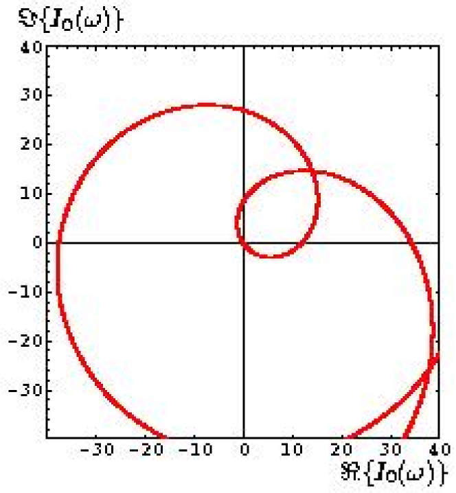
Figure 1: $I_{0}(\omega)$ in the complex plain for $\omega\in[0,\pi/t_{b}]$. The scale is arbitrary.

III Approximate Threshold Current

It can often be justified to linearize in $\epsilon=\frac{\omega_{\lambda}}{2Q_{\lambda}}t_{b}$, $\epsilon\ll 1$, which describes a situation when HOM decay is negligible on the time scale of the bunch spacing $t_{b}$. This applies to linacs when nearly every RF bucket is filled. The smallest $|I_{0}|$ in Eq. (18) is obtained when $\cos\omega t_{b}$ is close to $\cos\omega_{\lambda}t_{b}$, which occurs whenever $\omega$ is close to $\omega_{\lambda,n_{\pm}}=\pm\omega_{\lambda}+n\frac{2\pi}{t_{b}}$ for any integer $n$. Due to Eq. (21), all these frequencies lead to the same threshold current. We therefore additionally linearize in $\Delta\omega=\omega-\omega_{\lambda,n_{\pm}}$, assuming $\Delta\omega t_{b}\ll 1$. This leads to

$$I_{0}=\mp\frac{2}{\mathcal{K}T_{12}}e^{-i\omega n_{r}t_{b}}e^{i\omega_{\lambda,0\pm}\delta t_{b}}(\Delta\omega t_{b}+i\epsilon)\ .$$ (22)

Within the linearization, the phase factors could be combined to $e^{i\omega t_{r}}$. This is not done in order to retain the symmetries of Eq. (21) for $\omega\to\omega+2\pi/t_{b}$ and for $\omega\to-\omega^{*}$, i.e. $\Delta\omega\to-\Delta\omega^{*}$ and $\omega_{\lambda,n\pm}\to\omega_{\lambda,-n\mp}$.

Due to these symmetries, the real current close to $\omega_{\lambda,n\pm}$ is the same for each of these frequencies. Without loss of generality we therefore use $\omega_{\lambda,n\pm}=\omega_{\lambda}$ and no longer require the symmetries,

$$I_{0}=-\frac{2}{\mathcal{K}T_{12}}e^{-i\omega t_{r}}(\Delta\omega t_{b}+i\epsilon)\ .$$ (23)

Since $I_{0}$ must be real, $\Delta\omega t_{b}\sin\omega t_{r}=\epsilon\cos\omega t_{r}$ leading to the following two equivalent equations,

$$I_{0} = -\frac{\epsilon}{\mathcal{K}}\frac{2}{T_{12}\sin\omega t_{r}}\ ,$$ (24)

$$I_{0} = -{\rm sign}(\sin\omega t_{r})\frac{2}{\mathcal{K}T_{12}}\sqrt{\epsilon^{2}+(\Delta\omega t_{b})^{2}}\ .$$ (25)

For this formula to describe the threshold current, it is required that $I_{0}>0$ and therefore $T_{12}\sin\omega t_{r}<0$.

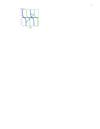
Figure 2: $\Delta\omega t_{b}$ (blue dots) and $\epsilon\cot\omega t_{r}$ (blue and green curves). The curve is dark blue in the region where $T_{12}\sin\omega t_{r}<0$ and light green otherwise. The $\omega$ of the instability is given by the intersection of the dotted line with a dark blue solid curve for which $\Delta\omega$ is smallest. Left: A case of $T_{12}\sin\omega_{\lambda}t_{r}<0$. Right: A case of $T_{12}\sin\omega_{\lambda}t_{r}>0$.

Figure 2 shows $\Delta\omega t_{b}$ and $\epsilon\cot\omega t_{r}$ versus $\omega t_{b}\in[0,\pi]$ for $t_{r}=6.88t_{b}$. The dotted line and the curve have to meet at a region where $T_{12}\sin\omega t_{t}<0$, which is indicated by a dark blue curve.

When $n_{r}\epsilon\ll 1$, i.e. HOM decay is negligible on the time scale of recirculation time, then $\omega\approx\omega_{\lambda}$ in the region where $T_{12}\sin\omega_{\lambda}t_{r}<0$ and one obtains

$$I_{0}=-\frac{\epsilon}{\mathcal{K}}\frac{2}{T_{12}\sin\omega_{\lambda}t_{r}}\ ,$$ (26)

which is the traditional and commonly used approximation in Eq. (1) which had been derived for $\delta=0$.

In the region with $T_{12}\sin\omega_{\lambda}t_{r}>0$ one obtains $\omega n_{r}\approx n\pi$, which can be used in Eq. (25),

$$I_{0}=\frac{2}{\mathcal{K}|T_{12}|}\sqrt{\epsilon^{2}+\frac{1}{n_{r}^{2}}{\rm Mod}(\omega_{\lambda}t_{r},\pi)^{2}}\ .$$ (27)

For $n_{r}\epsilon\gg 1$, i.e. when HOM damping is substantial on the recirculation time scale, one again uses Eq. (25) with $\omega t_{r}\approx(2n\mp\frac{1}{2})\pi$, where the $+$ or $-$ sign is determined by the sign of $T_{12}\sin\omega_{\lambda}t_{r}$,

$$I_{0}=\frac{2}{\mathcal{K}|T_{12}|}\sqrt{\epsilon^{2}+\frac{1}{n_{r}^{2}}{\rm Mod}(\omega_{\lambda}t_{r}\pm\frac{\pi}{2},2\pi)^{2}}\ .$$ (28)

Note that in this case the threshold current weakly depends on $t_{r}$ and can be estimated simply by $I_{0}=2\epsilon/\mathcal{K}|T_{12}|$.

One can perform these approximations more accurately, for example, by approximating $\cot\omega t_{r}$ by a line or second order curve. However, in regions where $n_{r}\epsilon$ is not much larger or much smaller than $1$, simple formulas cannot be found.

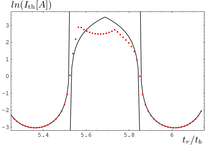
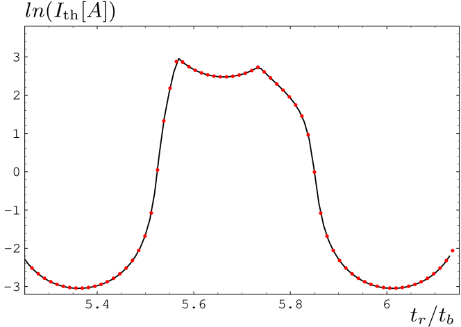
Figure 3: Threshold current obtained by tracking (red dots) and approximate analytical solution (top) and by a numerical solution (bottom) of the dispersion relation Eq. (18). Parameters: $n_{r}-\delta\in[6.135,7.234]$, $(R/Q)_{\lambda}=100\,\Omega$, $Q_{\lambda}=10^{4}$, $T_{12}=-10^{-6}$ eV/c, $\omega_{\lambda}t_{b}=9.67$.

Figure 3 (top) shows the threshold current obtained with the approximate analytic solution compared with the threshold current that is found by tracking particles for the simple case of one cavity with one HOM and one recirculation loop.

Figure 3 (bottom) compares the same tracking results with a numerical solution of the dispersion relation Eq. (18). The data agrees remarkably well with the approximate formula in the region where $\Delta\omega$ is small, i.e. where $I_{0}$ is relatively small. In the region where the threshold current is relatively large, the agreement with the approximate expression is not satisfactory, however.

To find the threshold current with Eq. (18), the smallest positive real value of $I_{0}$ for $\omega\in[0,\pi/t_{b}]$ was found by linearly interpolating 100 points in the region $\omega\in[\omega_{\lambda}-\frac{1}{n_{r}}\frac{\pi}{t_{b}},\omega_{\lambda}+\frac{1}{n_{r}}\frac{\pi}{t_{b}}]$.

III.1 Instability Growth Rate

We denote the threshold current by $\hat{I}_{0}$ and the real frequency $\hat{\omega}\in[0,\pi/t_{b}]$ satisfies Eq. (18) for this current. When the current $I_{0}$ is slightly larger than $\hat{I}_{0}$, there is one frequency $\omega(I_{0})$ that satisfies Eq. (18) and is close to $\hat{\omega}$. It has a positive imaginary part. All other frequencies $\omega$ at which Eq. (18) holds and for which therefore $\tilde{V}^{\Sigma}(\omega)$ might not vanish have an imaginary part that is not positive. In Eq. (10) there are therefore exponentially growing terms. For currents that are only slightly larger than the threshold current, the complex frequency $\omega(I_{0})$ can be expanded with respect to $\Delta I=I_{0}-\hat{I}_{0}$,

$$e^{-i\omega t}=e^{-i[\hat{\omega}+{\rm\Re}\{\frac{d\omega}{dI_{0}}\Delta I\}]t}e^{{\rm\Im}\{\frac{d\omega}{dI_{0}}\Delta I\}t}\ .$$ (29)

The rise time per current of the instability is thus given by $\alpha={\rm\Im}\{\frac{d\omega}{dI_{0}}\}|_{\hat{I}_{0}}$. The dispersion relation Eq. (18) leads to a long formula. However, using the simplified Eq. (22) leads to

$$\alpha = \left.\Im\big{\{}\frac{1}{dI_{0}/d\omega}\big{\}}\right|_{\hat{I}_{0}}$$

$$= \frac{1}{\hat{I}_{0}}\Im\big{\{}\big{(}-in_{r}t_{b}+\frac{t_{b}}{(\hat{\omega}-\omega_{\lambda})t_{b}+i\epsilon}\big{)}^{-1}\big{\}}\$$

$$= \frac{1}{\hat{I}_{0}t_{b}}\frac{4\epsilon+(\hat{I}_{0}\mathcal{K}T_{12})^{2}n_{r}}{4+8n_{r}\epsilon+(\hat{I}_{0}\mathcal{K}T_{12}n_{r})^{2}}\ .$$

Provided parameters are not in the region where the curves diverge in Fig. 3 (top), i.e. $\sin\omega_{\lambda}t_{r}$ is not close to zero, the following approximate formulas hold for the growth rate: For $n_{r}\epsilon\ll 1$ one obtains $\alpha=\frac{1}{\hat{I}_{0}t_{b}}\epsilon$ and for $n_{r}\epsilon\gg 1$ one obtains $\alpha=\frac{1}{\hat{I}_{0}t_{b}}\frac{1}{n_{r}}$.

IV Multiple Dipole HOMs and Multiple Recirculations

Recirculating linacs with many cavities and several recirculation loops have been considered early on Bisognano87_01 ; krafft89 . Here we use the same nomenclature as much as possible. The $N$ higher order modes, which can be associated with different cavities, are numbered by an index $i$. The $N_{p}$ passes through the linac are numbered by an index $I$. The horizontal position and momentum that the beam has at time $t$ in the HOM $i$ during turn $I$ is denoted $\vec{z}_{i}^{I}(t)=(x_{i}^{I}(t),p_{i}^{I}(t))$. The transport matrix that transports the phase space vector $\vec{z}_{j}^{J}$ at HOM $j$ during turn $J$ to $\vec{z}_{i}^{I}$ is denoted ${\bf T}_{ij}^{I\!J}$ and the time it takes to transport a particle from the beginning of the first turn to HOM $i$ during turn $I$ is denoted $t_{i}^{I}$. The beam is propagated from after HOM $i-1$ to after HOM $i$ by

$$\vec{z}_{i}^{I}(t)={\bf T}_{ii-1}^{II}\cdot\vec{z}_{i-1}^{I}(t-[t_{i}^{I}-t_{i-1}^{I}])+\left(\begin{array}[]{c}0\\ \frac{e}{c}V_{i}(t)\end{array}\right)\ .$$ (31)

This equation can be iterated to obtain the phase space coordinates as a function of the HOM strength that creates the orbit oscillations. With the matrix element $T_{ij}^{I\!J}=({\bf T}_{ij}^{I\!J})_{12}$ one obtains

$$x_{i}^{I}(t) = \sum_{J=1}^{I-1}\sum_{j=1}^{N}T_{ij}^{I\!J}\frac{e}{c}V_{j}(t-[t_{i}^{I}-t_{j}^{J}])$$

$$+ \phantom{\sum_{J=1}^{I-1}}\sum_{j=1}^{i-1}T_{ij}^{II}\frac{e}{c}V_{j}(t-[t_{i}^{I}-t_{j}^{I}])\ .$$

The strength $V_{i}(t)$ of the HOM $i$ is created by all particles that have traveled through that HOM via the integral

$$V_{i}(t)=\int_{-\infty}^{t}\sum_{I=1}^{N_{p}}W_{i}(t-t^{\prime})I_{i}^{I}(t^{\prime})x_{i}^{I}(t^{\prime})dt^{\prime}\ ,$$ (33)

where $I_{i}^{I}(t)$ is the current at time $t$ that the fraction of the beam has which passes the HOM $i$ on turn $I$. Combining this with Eq. (IV) leads to the following integral-difference equation:

$$V_{i}(t) = \int_{-\infty}^{t}\sum_{I=1}^{N_{p}}W_{i}(t-t^{\prime})I_{i}^{I}(t^{\prime})$$

$$\times \frac{e}{c}\sum_{J=1}^{I}\sum_{j=1}^{N_{I\!J}(i-1)}T_{ij}^{I\!J}V_{j}(t^{\prime}-[t_{i}^{I}-t_{j}^{J}])dt^{\prime}\ ,$$

$$N_{I\!J}(i-1) = \begin{cases}N,&\text{if $I\neq J$;}\\ i-1,&\text{if $I=J$.}\end{cases}$$ (35)

Now the approximation of short bunches is used. The current is given at time $t$ by pulses that are equally spaced with the distance $t_{b}$,

$$I_{i}^{I}(t)=\sum_{m=-\infty}^{\infty}I_{0}t_{b}\delta(t-t_{i}^{I}-mt_{b})\ .$$ (36)

This reduces the integral to a sum,

$$V_{i}(t) = \frac{e}{c}I_{0}t_{b}\sum_{m=-\infty}^{n(t,t_{i}^{I})}\sum_{I=1}^{N_{p}}W_{i}(t-t_{i}^{I}-mt_{b})$$

$$\times \sum_{J=1}^{I}\sum_{j=1}^{N_{I\!J}(i-1)}T_{ij}^{I\!J}V_{j}(mt_{b}+t_{j}^{J})\ ,$$

where $n(t,t_{i}^{I})={\rm Max}_{m}(t\geq mt_{b}+t_{i}^{I})$. Computing

$$V_{i}^{L}=\sum_{n=-\infty}^{\infty}V_{i}(nt_{b}+t_{i}^{L})e^{i\omega nt_{b}}$$ (38)

leads to

$$V_{i}^{L} = \frac{e}{c}I_{0}t_{b}\sum_{n=-\infty}^{\infty}\sum_{m=m^{*}}^{\infty}\sum_{I=1}^{N_{p}}W_{i}(mt_{b}+t_{i}^{L}-t_{i}^{I})$$

$$\times \sum_{J=1}^{I}\sum_{j=1}^{N_{I\!J}(i-1)}T_{ij}^{I\!J}V_{j}([n-m]t_{b}+t_{j}^{J})e^{i\omega nt_{b}}\ .$$

The second summation starts at $m^{*}=n-n(nt_{b}+t_{i}^{L},t_{i}^{I})$ which can be simplified by writing $t_{i}^{I}=(n_{i}^{I}-\delta_{i}^{I})t_{b}$,

$$m^{*} = n-n([n+n_{i}^{L}-n_{i}^{I}]t_{b},[\delta_{i}^{-}\delta_{i}^{I}]t_{b})$$

$$= -{\rm Max}_{m}([n_{i}^{L}-n_{i}^{I}]t_{b}\geq[m+\delta_{i}^{L}-\delta_{i}^{I}]t_{b})$$

$$= n_{i}^{I}-n_{i}^{L}+\gamma_{i}(I,L)\ ,$$

where $\gamma_{i}(I,L)=1$ if $\delta_{i}^{L}>\delta_{i}^{I}$ and $0$ otherwise. Shifting the summation index $m$ now leads to

$$V_{i}^{L} = \frac{e}{c}I_{0}t_{b}\sum_{n=-\infty}^{\infty}\sum_{m=0}^{\infty}\;\>\sum_{I=1}^{N_{p}}$$

$$W_{i}([m+\gamma_{i}(I,L)+\delta_{i}^{I}-\delta_{i}^{L}]t_{b})\sum_{J=1}^{I}\sum_{j=1}^{N_{I\!J}(i-1)}T_{ij}^{I\!J}$$

$$\times V_{j}([n-m-n_{i}^{I}+n_{i}^{L}-\gamma_{i}(I,L)]t_{b}+t_{j}^{J})e^{i\omega nt_{b}}\ .$$

and with $\delta_{i}(I,L)=\gamma_{i}(I,L)+\delta_{i}^{I}-\delta_{i}^{L}$, which is between $0$ and $1$, shifting the index $n$ finally leads to the relation

$$V_{i}^{L} = \frac{e}{c}I_{0}t_{b}\sum_{m=0}^{\infty}\sum_{I=1}^{N_{p}}W_{i}([m+\delta_{i}(I,L)]t_{b})$$

$$\times \sum_{J=1}^{I}\sum_{j=1}^{N_{I\!J}(i-1)}T_{ij}^{I\!J}e^{i\omega[m+n_{i}^{I}-n_{i}^{L}+\gamma_{i}(I,L)]t_{b}}V_{j}^{J}\ .$$

The following sum is equivalent to that in Eq. (II.2),

$$w_{i}(\delta)=\sum_{m=0}^{\infty}W_{i}([m+\delta]t_{b})e^{i\omega mt_{b}}\ .$$ (43)

Equation (IV) reduces to

$$\frac{1}{I_{0}}V_{i}^{L} = \frac{e}{c}t_{b}\sum_{I=1}^{N_{p}}w_{i}(\delta_{i}(I,L))e^{i\omega(t_{i}^{I}-t_{i}^{L}+\delta_{i}(I,L)t_{b})}$$ (44)

$$\times \sum_{J=1}^{I}\sum_{j=1}^{N_{I\!J}(i-1)}T_{ij}^{I\!J}V_{j}^{J}\ .$$

If a vector $\vec{V}$ is introduced that has the coefficients $V_{i}^{I}$, this equation can be written in matrix form,

$$\frac{1}{I_{0}}\vec{V}={\bf W}(\omega){\bf U}\vec{V}\ ,$$ (45)

where the matrix ${\bf M}={\bf W}(\omega){\bf U}$ is determined by Eq. (44). When all electrons are considered to have the speed of light, $t_{i}^{I}-t_{i}^{L}$ does not depend on the HOM number $i$ and we therefore drop this index and obtain the following matrix coefficients:

$$M_{ij}^{LJ} = \frac{e}{c}t_{b}\sum_{I=J+\Theta_{j,i}}^{N_{p}}w_{i}(\delta(I,L))e^{i\omega{\rm Top}(\frac{t^{I}-t^{L}}{t_{b}})t_{b}}T_{ij}^{I\!J}$$

$$\Theta_{j,i} = \begin{cases}1,&\text{if $j\geq i$;}\\ 0,&\text{otherwise,}\end{cases}$$ (46)

where ${\rm Top}(x)$ is the smallest integer that is equal to or larger than $x$. With Kronecker $\hat{\delta}_{ik}$ this determines the matrices ${\bf W}$ and ${\bf U}$ to be

$$W_{ik}^{LI} = \frac{e}{c}t_{b}w_{i}(\delta(I,L))e^{i\omega{\rm Top}(\frac{t^{I}-t^{L}}{t_{b}})t_{b}}\delta_{ik}\ ,$$ (47)

$$U_{kj}^{I\!J} = T_{kj}^{I\!J}\Theta_{I,J+\Theta_{j,k}}\ .$$ (48)

For each frequency $\omega$, $I_{0}^{-1}$ is an eigenvalue of ${\bf M}(\omega)$. Since the eigenvalues are in general complex, but $I_{0}$ has to be real, the threshold current is determined by the largest real eigenvalue of ${\bf M}(\omega)$. The matrix has the properties

$${\bf M}(\omega+\frac{2\pi}{t_{b}})={\bf M}(\omega)\ ,\ \ {\bf M}(-\omega^{*})={\bf M}^{*}(\omega)\ ,$$ (49)

and it is therefore again sufficient to investigate $\omega\in[0,\pi/t_{b}]$ to find the threshold current.

Note that $V_{N}^{N_{p}}$ never appears on the right hand side of Eq. (IV) so that the dimension of ${\bf M}$ can be reduced by one to $N\times N_{p}-1$. Furthermore the dimension can be reduced when two fractional parts $\delta_{i}^{I}$ and $\delta_{j}^{J}$ are equal since then $V_{i}^{I}$ and $V_{j}^{J}$ are identical. Note also that for $N=1$ and $N_{p}=2$ Eq. (IV) reduces to the dispersion relation for one HOM in Eq. (18).

IV.1 Instability Growth Rate

The growth rate of the instability is again computed by first obtaining the threshold current $\hat{I}_{0}$ and the real frequency $\hat{\omega}$ for which $\hat{I}_{0}^{-1}$ is an eigenvalue of ${\bf M}(\hat{\omega})$. If this is the $k$th eigenvalue $\lambda_{k}(\omega)$ of the matrix ${\bf M}(\omega)$, then the growth rate of the instability is given by

$$\alpha=-{\hat{I}}_{0}^{-2}\left.\Im\big{\{}\big{(}\frac{d\lambda_{k}}{d\omega}\big{)}^{-1}\big{\}}\right|_{I_{0}=\hat{I}_{0}}\ .$$ (50)

V Multiple HOMs in one Cavity

The presented theory for multiple HOMs and multiple recirculation turns can in general only be evaluated with computers. However, for some simple situation an analytical understanding is possible.

One such case is an accelerator with one recirculation loop and one cavity in which many HOMs can be excited. The $(1,2)$ matrix elements that refer to transport between HOMs for the same pass are zero, $T^{J\!J}_{ij}=0$. All matrix elements that describe the recirculation loop are identical, $T^{I\!J}_{ij}=T_{12}$ if $I\neq J$. The matrix elements in Eq. (46) are then given by

$$M^{L2}_{ij}=0\ ,\\ M^{L1}_{ij}=\frac{e}{c}t_{b}w_{i}(\delta(2,L))e^{i\omega{\rm Top}(\frac{t^{2}-t^{L}}{t_{b}}t_{b})}T_{12}\ .$$ (51)

Equation (45) becomes with $\delta=\delta(2,1)$,

$$\frac{1}{I_{0}}V^{1}_{i}=\frac{e}{c}t_{b}\sum_{j}w_{i}(\delta)e^{i\omega n_{r}t_{b}}T_{12}V^{1}_{j}\ .$$ (52)

A summation over the index $i$ shows that $\sum_{j}V^{1}_{j}$ can only be nonzero when

$$\frac{1}{I_{0}}=t_{b}T_{12}\frac{e}{c}e^{i\omega n_{r}t_{b}}\sum_{i}w_{i}(\delta)\ .$$ (53)

Comparing this with Eq. (14) shows that one only has to replace $w(\delta)$ of the single HOM by $\sum_{i}w_{i}(\delta)$ to arrive at the threshold formula for the multi-HOM case. To find the smallest real $I_{0}$ that Eq. (53) can produce for real $\omega$, $\sum_{i}w_{i}(\delta)$ has to be maximized. The sum is especially large when the denominator of one of the terms is very small, i.e. when $\cos\omega t_{b}\approx\cos\omega_{\lambda}t_{b}$.

When the HOM frequencies modulo $2\pi/t_{b}$ are sufficiently different for the different HOMs, the maximal absolute value of $\sum_{i}w_{i}(\delta)$ will be close to the largest absolute value that any of the $w_{i}(\delta)$ could have individually. This is due to the fact that all the $w_{j}(\delta)$ for $j\neq i$ are relatively small for frequencies $\omega$ for which the denominator of $w_{i}(\delta)$ is small.

For HOM frequencies that are sufficiently different in the above sense, the threshold current for several HOMs therefore does not differ significantly from the threshold current of the worst individual HOM.

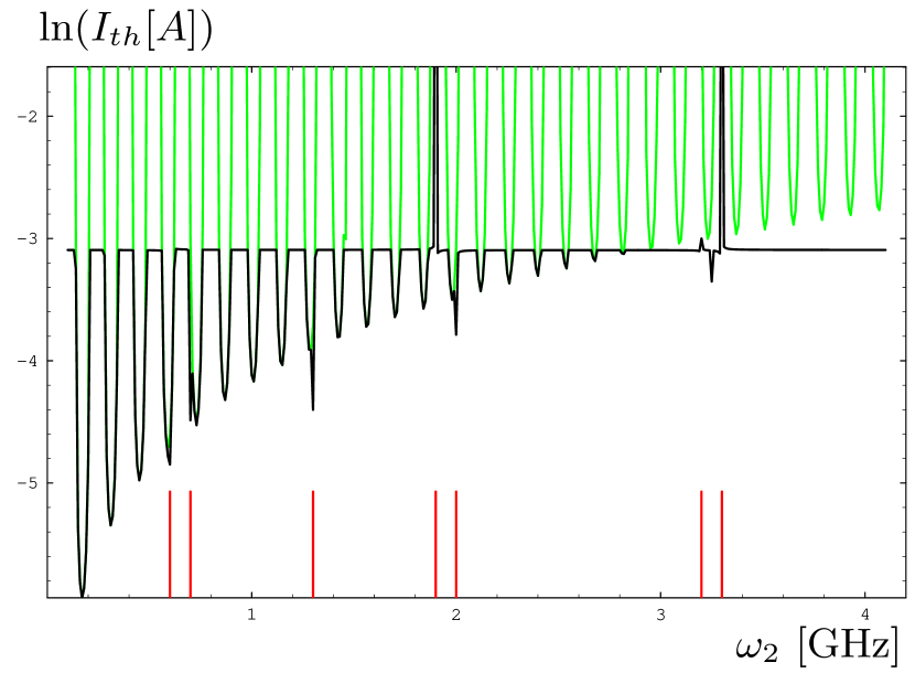
Figure 4: Dark black curve: the threshold current $\ln(I_{th}{\rm[A]})$ for one HOM at $\omega_{1}/2\pi=2\,$GHz as a function of a second HOM with frequency $\omega_{2}$. Light green curve: threshold current when only the second HOM is present. Light red lines: frequencies for which $\cos\omega_{2}t_{b}\approx\cos\omega_{1}t_{b}$ where the threshold current is not simply the minimum of the threshold currents produced by the individual HOMs.

Figure 4 shows how the threshold current changes when the frequency of one HOM is fixed at a small threshold current with $|\sin\omega_{1}t_{r}|=1$ and a second HOM frequency is varied. Superimposed is $I_{th}$ if only the second HOM is present. It is apparent that the HOM that would produce the larger threshold-current if it was solely present only influences the threshold current of the pair when the frequencies $\pm\omega_{1}\,{\rm mod}\,2\pi/t_{b}$ and $\pm\omega_{2}\,{\rm mod}\,2\pi/t_{b}$ are closer together than about $\Delta\omega_{\lambda}=\epsilon/t_{b}=\omega_{\lambda}/2Q_{\lambda}$.

One can draw the conclusion that in the case of many HOMs they do not interact destructively when the frequencies $\pm\omega_{\lambda}\,{\rm mod}\,2\pi/t_{b}$ are not very close together. Tracking simulations also demonstrate this effect.

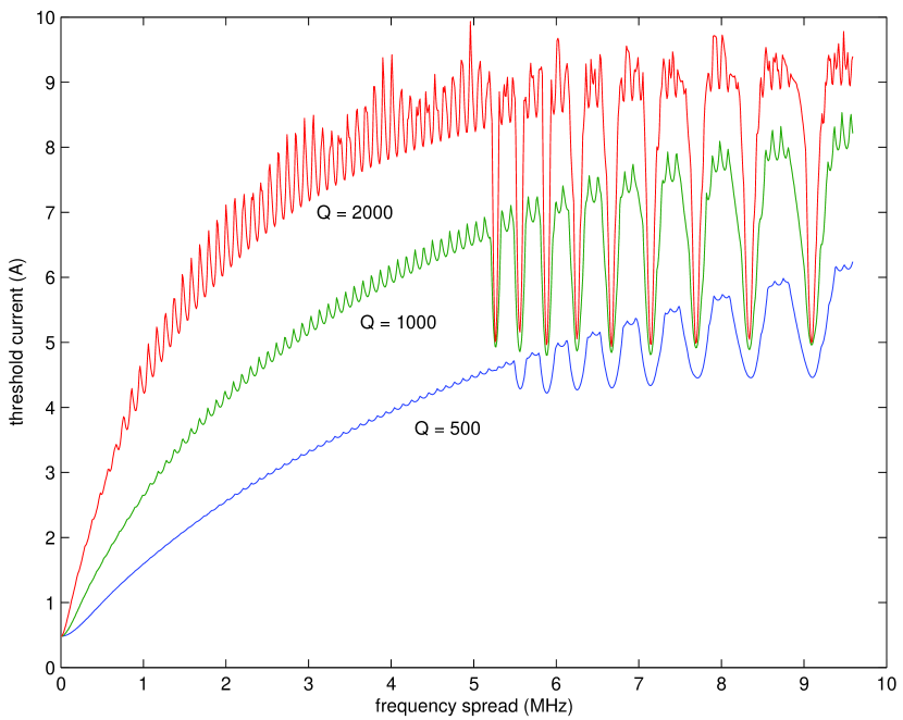
Figure 5: The threshold current $I_{th}$ as a function of uniform equidistant frequency spread for 20 HOMs in a single cavity. Abscissa displays frequency difference between the two HOMs adjacent in frequency. Parameters: $\bar{\omega}_{\lambda}/2\pi=2\,$GHz, $(R/Q)_{\lambda}Q_{\lambda}=5000\,\Omega$, $T_{12}=-10^{-6}\,$eV/c, $t_{r}=1.000125\cdot 10^{-6}\,$s, $\omega_{0}/2\pi=1.3\,$GHz. Threshold is determined by tracking with accuracy $0.1\%$.

One strategy to increase the BBU threshold current is the introduction of HOM frequency spreads between cavities. As an example, Fig. 5 shows the threshold current found by tracking as a function of uniform frequency spread of 20 HOMs in a single cavity. For all three curves $(R/Q)_{\lambda}Q_{\lambda}$ is the same. It is seen that for lower $Q_{\lambda}$, the curve begins to saturate for larger frequency spread than for the high $Q_{\lambda}$ case. It is also seen that the threshold for frequency spread $\omega_{\lambda}/2Q_{\lambda}$ is similar in all three cases. Both observations are consistent with the above assertion that HOMs do not interfere when they are further apart than $\omega_{\lambda}/2Q_{\lambda}$. The fact that oscillations in the Fig. 5 are smaller for low $Q_{\lambda}$ is consistent with the conclusion that a broader HOM resonance peak should lead to more overlaps and as a result to less pronounced differences in the threshold for different HOM frequencies.

VI One Dipole HOM in Two Cavities

In order to see how two dipole HOMs interact, we will now analyze a set of two HOMs with one recirculation loop, i.e. $N_{p}=2$. We abbreviate $\delta=\delta(2,1)$ and $\alpha_{r}=e^{i\omega n_{r}t_{b}}$. The dispersion relation is then given by

$$\frac{1}{I_{0}}\left(\begin{array}[]{c}V_{1}^{1}\\ V_{2}^{1}\\ V_{1}^{2}\end{array}\right)=\frac{e}{c}t_{b}{\bf N}\left(\begin{array}[]{c}V_{1}^{1}\\ V_{2}^{1}\\ V_{1}^{2}\end{array}\right)$$ (54)

where the matrix ${\bf N}$ is given by

$$\left(\begin{array}[]{ccc}w_{1}(\delta)\alpha_{r}T_{11}^{21}&w_{1}(\delta)\alpha_{r}T_{12}^{21}&0\\ w_{2}(0)T_{21}^{11}+w_{2}(\delta)\alpha_{r}T_{21}^{21}&w_{2}(\delta)\alpha_{r}T_{22}^{21}&w_{2}(\delta)\alpha_{r}T_{21}^{22}\\ w_{1}(0)T_{11}^{21}&w_{1}(0)T_{12}^{21}&0\end{array}\right)\ .$$ (55)

The third row is similar to the first row and eliminating it by similarity transformations leads to the $2\times 2$ matrix

$$\left(\begin{array}[]{cc}w_{1}(\delta)\alpha_{r}&0\\ 0&w_{2}(\delta)\alpha_{r}\end{array}\right)\times$$ (58)

$$\left(\begin{array}[]{ccc}T_{11}^{21}&T_{12}^{21}\\ \frac{w_{2}(0)}{w_{2}(\delta)\alpha_{r}}T_{21}^{11}+T_{21}^{21}+\frac{w_{1}(0)}{w_{1}(\delta)\alpha_{r}}T_{21}^{22}&T_{22}^{21}\\ \end{array}\right)\ .$$ (61)

Even though $\omega_{1}(\delta)$ appears in the denominator, the formula for the eigenvalues of this matrix does not contain such a denominator. Therefore the largest real eigenvalue will again occur at a frequency $\omega$ for which one of the HOM frequencies satisfies $\cos(\omega t_{b})\approx\cos(\omega_{\lambda}t_{b})$. The term $w_{i}(\delta)$ and $w_{i}(0)$ of the other HOM can then again be neglected, so that for sufficiently different HOM frequencies ${\rm mod}\>2\pi/t_{b}$ the threshold current is again approximately determined by the HOM which would have the smallest $I_{th}$ if there were no other HOMs present.

We therefore now assume that the two HOMs are equal, $w_{1}=w_{2}$. Now one can perform an approximation analogous to Eq. (23) leading to

$${\bf N}=-\frac{\mathcal{K}}{2}e^{i\omega t_{r}}\frac{1}{\Delta\omega t_{b}+i\epsilon}\times$$ (62)

$$\left(\begin{array}[]{cc}T_{11}^{21}&T_{12}^{21}\\ T_{21}^{21}+e^{-i\omega t_{r}}(T_{21}^{11}+T_{21}^{22})&T_{22}^{21}\end{array}\right)\ .$$ (65)

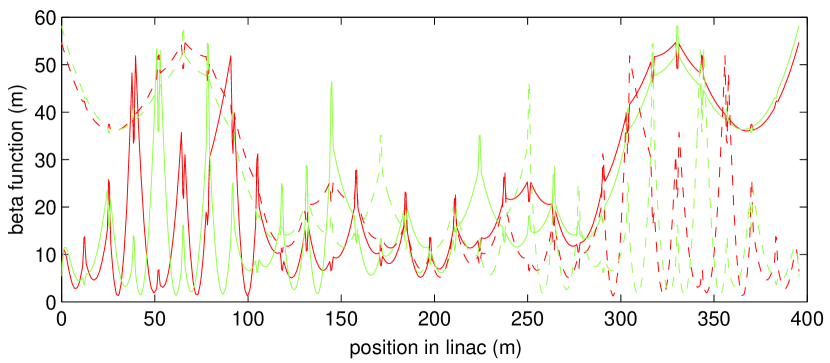
Figure 6: Example of a mirror-symmetric linac optics. Dark red curve (light green curve) is horizontal (vertical) beta function in the linac for accelerating beam. Dashed lines show lattice function for decelerating beam.

It is interesting to analyze whether the effect of the two HOMs can cancel. A cancellation could occur most naturally when the linac and the recovery loop are mirror symmetric. A mirror symmetry of the linac means that the beta functions of the first pass, going from low to high energy, are the mirror image of those of the second pass, going from high to low energy. An example of such an optics is shown in Fig. 6.

Since the $(1,2)$ element of the transport matrix between a region with momentum $p_{0}$ and a region with momentum $p$ can be written with Twiss parameters as

$$T_{12}=\sqrt{\frac{\beta\beta_{0}}{pp_{0}}}\sin\Delta\Psi\ ,$$ (66)

this symmetry leads to $T_{21}^{22}=T_{21}^{11}$. An additional mirror symmetry of the return arc leads to $T_{22}^{21}=T_{11}^{21}$. The eigenvalues of the matrix in Eq. (62) then become,

$$\frac{1}{I_{0}} = -\frac{\mathcal{K}}{2}e^{i\omega t_{r}}\frac{1}{\Delta\omega t_{b}+i\epsilon}\times$$

$$\left[T_{11}^{21}\pm\sqrt{T_{12}^{21}(T_{21}^{21}+2e^{-i\omega t_{r}}T_{21}^{11})}\right]\ .$$

Since there are two solutions to the quadratic eigenvalue equation, to every eigenvalue that is smaller than $1/I_{\rm th}$ of a single cavity, there exists in general the one that is larger. Therefore two cavities do not compensate their instabilities, but it is possible to decouple the cavities to the extent that the combined threshold current is just as large as that for a single cavity. For this, one has to choose $T_{12}^{21}=0$, i.e. the phase advance of the return arc has to be a multiple of $\pi$.

Since the kick of a HOM disturbs the beam most at low energy, the first and the last cavity of an ERL are the strongest contributors to BBU. It seems therefore advisable to adjust the phase advance of the arc to a multiple of $\pi$ also when the linac has more than two cavities.

VI.1 Multiple Recirculation Turns

One could envision a multi-turn recirculating linac as ERL. The beam would pass the same linac $N_{r}$ times to reach its top energy, and subsequently it would be decelerated in just as many turns through the linac. The current in the cavities would be $2N_{r}$ times higher than the current that is available at high energy. One could therefore conjecture that the BBU threshold current is $N_{r}$ times smaller than for a one-turn ERL. Here we will show that the threshold current can be significantly smaller than that conjecture and in general can be expected to decrease quadratically with $N_{r}$.

Each bunch passes the linac $N_{p}=2N_{r}$ times and the matrix in Eq. (46) becomes

$$M^{LJ}=\frac{e}{c}t_{b}\sum_{I=J+1}^{N_{p}}w(\delta(I,L))e^{i\omega{\rm Top}(\frac{t^{I}-t^{L}}{t_{b}})t_{b}}T^{I\!J}\ ,$$ (68)

where the lower indexes have been suppressed since only one HOM is considered. The eigenvalue equation thus becomes

$$\frac{1}{I_{0}}V^{L}=\frac{e}{c}t_{b}\sum_{J=1}^{N_{p}}\sum_{I=J+1}^{N_{p}}w(\delta(I,L))e^{i\omega{\rm Top}(\frac{t^{I}-t^{L}}{t_{b}})t_{b}}T^{I\!J}V^{J}\ ,$$ (69)

An approximation equivalent to that leading to Eqs. (23) and (62) results in

$$\frac{1}{I_{0}}V^{L}=-\frac{\mathcal{K}}{2}\frac{1}{\Delta\omega t_{b}+i\epsilon}\times$$ (70)

$$\sum_{J=1}^{N_{p}}\sum_{I=J+1}^{N_{p}}e^{i\omega[{\rm Top}(\frac{t^{I}-t^{L}}{t_{b}})-\delta(I,L)]t_{b}}T^{I\!J}V^{J}\ .$$

Comparing the exponent on the right hand side to those in Eqs. (44) and (46) shows that this can be written as

$$\frac{1}{I_{0}}V^{L}e^{i\omega t^{L}}=-\frac{\mathcal{K}}{2}\frac{1}{\Delta\omega t_{b}+i\epsilon}\times$$ (71)

$$\sum_{J=1}^{N_{p}}\sum_{I=J+1}^{N_{p}}e^{i\omega(t^{I}-t^{J})}T^{I\!J}V^{J}e^{i\omega t^{J}}\ .$$

Since the right hand side does not depend on $L$, all the terms $V^{J}e^{i\omega t^{J}}$ are equivalent and the condition that they do not vanish is

$$\frac{1}{I_{0}}=-\frac{\mathcal{K}}{2}\frac{1}{\Delta\omega t_{b}+i\epsilon}\sum\!\!\!\!\!\!\!\!\sum\limits_{I>J}e^{i\omega(t^{I}-t^{J})}T^{I\!J}\ ,$$ (72)

where the double sum goes over all pairs of $I$ and $J$ for which $I>J$. Similar to the condition obtained from Eq. (23) which is analyzed with Fig. 2, the fact that $I_{0}$ has to be real entails the condition

$$\frac{\sum\!\!\!\!\!\!\!\!\sum\limits_{I>J}\cos(\omega[t^{I}-t^{J}])T^{I\!J}}{\sum\!\!\!\!\!\!\!\!\sum\limits_{I>J}\sin(\omega[t^{I}-t^{J}])T^{I\!J}}=\frac{\Delta\omega}{\epsilon}\ .$$ (73)

In regions where $\sum\!\!\!\!\!\!\!\!\sum_{I>J}\sin(\omega[t^{I}-t^{J}])T^{I\!J}>0$, we again obtain the approximation that $\omega\approx\omega_{\lambda}$. The equation for the threshold current of an $N_{r}$ times recirculating ERL $I_{\rm th}^{N_{r}}$ corresponds therefore to that of the case without recirculation in Eq. (1),

$$I_{th}^{N_{r}}=-\frac{2c^{2}}{e(\frac{R}{Q})_{\lambda}Q_{\lambda}\omega_{\lambda}}\frac{1}{\sum\!\!\!\!\!\!\!\!\sum\limits_{I>J}\sin(\omega[t^{I}-t^{J}])T^{I\!J}}\ .$$ (74)

A comparison with Eq. (1) shows that this current is smaller than the one-turn ERL by a factor of up to $\sum\!\!\!\!\!\!\!\!\sum_{I>J}|T^{I\!J}|/|T_{12}|$. This is in agreement with earlier result presented in randbook . Assuming that all matrix elements are of about equal magnitude, the threshold current in an $N_{r}$ times recirculating ERL is therefore in general smaller by about a factor of $N_{r}(2N_{r}-1)$. This conclusion is consistent with tracking results for microtrons microtron and for two-turn ERL twopassmemo . The scaling in a particular case, however, can be quite different depending on details of the lattice design, e.g. approximate scaling with $N_{r}$ was reported in hermin .

VII Cavity Misalignments

In the derivation above, it was assumed that the bunches travel along the cavities’ symmetry axes when the current is below the threshold for BBU instability. When the cavities are misaligned, the beam will excite dipole higher order modes even below the threshold and the trajectory will be disturbed by these modes.

Let us assume that the $i$th cavity is misaligned with respect to the path adjustment of the $I$th turn by $x_{0i}^{I}$, leading to the misalignment vector $\vec{x}_{0}$. The dipole HOMs that are excited by the beam are now not only due to the beam position fluctuation that is produced by the HOMs themselves, but additionally due to the cavity misalignments. The HOM voltages in Eq. (33) are therefore given by

$$V_{i}(t)=\int_{-\infty}^{t}\sum_{I=1}^{N_{p}}W_{i}(t-t^{\prime})I_{i}^{I}(t^{\prime})[x_{i}^{I}(t^{\prime})-x_{0i}^{I}]dt^{\prime}\ .$$ (75)

With the manipulations that led to Eq. (IV) this leads to

$$V_{i}(t) = I_{0}t_{b}\sum_{m=-\infty}^{n(t,t_{i}^{I})}\sum_{I=1}^{N_{p}}W_{i}(t-t_{i}^{I}-mt_{b})$$

$$\times \left[\sum_{J=1}^{I}\sum_{j=1}^{N_{I\!J}(i-1)}T_{ij}^{I\!J}\frac{e}{c}V_{j}(mt_{b}+t_{j}^{J})-x_{0i}^{I}\right]\ .$$

Following the derivation to Eq. (44) leads to

$$V_{i}^{L} = I_{0}t_{b}\sum_{I=1}^{N_{p}}w_{i}(\delta_{i}(I,L))e^{i\omega(t_{i}^{I}-t_{i}^{L}+\delta_{i}(I,L)t_{b})}$$ (77)

$$\times \left[\sum_{J=1}^{I}\sum_{j=1}^{N_{I\!J}(i-1)}T_{ij}^{I\!J}\frac{e}{c}V_{j}^{J}-x_{0i}^{I}\sum_{n=-\infty}^{\infty}e^{i\omega nt_{b}}\right]\ .$$

For all oscillation frequencies that are not multiples of the bunch repetition frequency, $\omega=2\pi l/t_{b}$, $l$ is an integer, the term $x_{0i}^{I}\sum_{n=-\infty}^{\infty}e^{i\omega nt_{b}}$ vanishes so that the condition for $V_{i}^{L}(\omega)$ to be non-zero is the same as for the BBU instability without misalignments $x_{0i}^{I}$. Below threshold, the HOM voltage therefore has the following form:

$$V_{i}(t)=\sum_{l=-\infty}^{\infty}V_{l}e^{i\frac{2\pi}{t_{b}}lt}\ .$$ (78)

The voltage seen by bunch $i$ on turn $L$ is therefore given by $\bar{V}_{i}^{L}=\sum_{l=-\infty}^{\infty}V_{l}e^{i\frac{2\pi}{t_{b}}lt_{i}^{L}}$ so that for the time $t_{i}^{L}$, Eq. (VII) can be written as

$$\bar{V}_{i}^{L} = I_{0}t_{b}\sum_{m=-\infty}^{n(t_{i}^{L},t_{i}^{I})}\sum_{I=1}^{N_{p}}W_{i}(t_{i}^{L}-t_{i}^{I}-mt_{b})$$

$$\times \left[\sum_{J=1}^{I}\sum_{j=1}^{N_{I\!J}(i-1)}T_{ij}^{I\!J}\frac{e}{c}\bar{V}_{j}^{J}-x_{0i}^{I}\right]\ .$$

After performing the summation over $m$ one obtains

$$\bar{V}_{i}^{L} = I_{0}t_{b}\sum_{I=1}^{N_{p}}w_{i}^{\omega=0}(\delta(I,L))$$

$$\times \left[\sum_{J=1}^{I}\sum_{j=1}^{N_{I\!J}(i-1)}T_{ij}^{I\!J}\frac{e}{c}\bar{V}_{j}^{J}-x_{0i}^{I}\right]\ ,$$

where the superscript $\omega=0$ means that $w(\delta)$ is computed with Eq. (II.2) for $\omega=0$.

Comparing with Eqs. (44) and (45) shows that this can be written as

$$\vec{\bar{V}}=I_{0}{\bf W}(0){\bf U}\vec{\bar{V}}-I_{0}{\bf W}(0)\vec{x}_{0}\ ,$$ (81)

with ${\bf W}={\bf W}(0)$ and ${\bf U}$ from Eqs. (47) and (48). The vector of voltages is therefore given by $\vec{\bar{V}}=[I_{0}{\bf WU}-{\bf I}]^{-1}I_{0}{\bf W}\vec{x}_{0}$. Equation (IV) can now be used to compute the beams distance from the cavity center at each turn and each cavity. One obtains

$$x_{i}^{I}(t_{i}^{I})-x_{0i}^{I} = \sum_{J=1}^{I}\sum_{j=1}^{N_{I\!J}(i-1)}T_{ij}^{I\!J}\frac{e}{c}\bar{V}_{j}^{J}-x_{0i}^{I}\ ,$$ (82)

$$\vec{x}-\vec{x}_{0} = {\bf U}[I_{0}{\bf WU}-{\bf I}]^{-1}I_{0}{\bf W}\vec{x}_{0}-\vec{x}_{0}$$

$$= [I_{0}{\bf UW}-{\bf I}]^{-1}\vec{x}_{0}\ .$$

Evaluating this for a single cavity with a single HOM leads to

$$x-x_{0}=\frac{x_{0}}{\frac{e}{c}I_{0}t_{b}T_{12}w^{\omega=0}(\delta)-1}\ .$$ (84)

For $\delta=\frac{1}{2}$ and with $\epsilon=\frac{\omega_{\lambda}}{2Q_{\lambda}}t_{b}$ one obtains

$$x-x_{0}=x_{0}\left[I_{0}\mathcal{K}T_{12}\frac{\cosh\frac{\epsilon}{2}\sin\frac{\omega_{\lambda}t_{b}}{2}}{\cosh\epsilon-\cos\omega_{\lambda}t_{b}}-1\right]^{-1}\ .$$ (85)

There is a current $I_{0}$ at which the denominator becomes $0$ and the orbit deviation would become very large. The question arises whether this current is larger than the BBU threshold $I_{\rm th}$ or smaller, so that large orbit excursions would present a new kind of instability.

This problem does not only arise for the single HOM case of Eq. (VII) but also for the general case of Eq. (85). Very large orbit excursions $x$ occur for currents for which the matrix inverse does not exist.

The inverse matrix to be inverted is $(I_{0}{\bf WU}-{\bf 1})^{-1}=I_{0}{\bf A}\,{\rm Diag}[(\lambda_{i}-1/I_{0})^{-1}]\,{\bf A}^{-1}$, where ${\bf A}$ is the matrix that diagonalizes ${\bf W}(0){\bf U}$. We therefore see that $1/I_{0}$ for which the orbit gets very large is given by the eigenvalues of ${\bf W}(0){\bf U}$. These values are naturally smaller than $1/I_{\rm th}$, which is the largest eigenvalue of ${\bf W}(\omega){\bf U}$ that is produced for any frequency $\omega$.

This proves that the BBU instability always occurs before the orbit excursion becomes very large.

VIII Tracking Results

The tracking code BI (stands for beam instability) was developed to perform studies of beam breakup in recirculating linacs bbucode . The algorithm models point charge bunch interactions with HOMs in linacs, taking into account proper time delays between the cavities, transfer maps, etc., allowing BBU simulations due to longitudinal, transverse and other higher order modes in a general linac configuration.

The basic algorithm can be summarized as following. The string of HOMs that a bunch sees in its lifetime between injection and ejection points is represented by a list of pointers to the actual cavities. The proper time delays between cavities is also stored for each pointer. E.g. for $N$ HOMs and $N_{p}$ passes, the list of pointers would be $NN_{p}$ long pointing to $N$ HOMs. This approach allows one to represent any recirculation configuration without limitations. As the train of bunches is injected into the structure, the next instance when any bunch sees any pointer is determined, and the HOM voltage in the corresponding cavity is updated. Then, this bunch is pushed to the next pointer where its coordinates are stored, waiting for its turn in time to be the next bunch going through a pointer. This way no bunches end up ahead of time precluding a situation when a bunch sees a cavity with incorrectly updated HOM fields, i.e. causality is properly realized. Furthermore, the algorithm is general enough to allow modeling of the longitudinal instability where timing between different bunches is no longer kept fixed. The practical realization of this algorithm is relatively fast, allowing the tracking of a complete $5\,$GeV ERL with $300$ HOMs for $0.1\,$ms in less than a minute on an average personal computer. This duration is sufficient to determine the onset of transverse BBU instability in most practical cases.

The output of the code contains amplitudes of HOM voltages as a function of time, which is used to determine the growth rate of the instability by fitting an exponential. Several successive calls are made to the tracking unit to determine the threshold. The length of the tracking time is estimated from Eq. (III.1) based on the desired accuracy in threshold determination.

IX Conclusion

For dipole HOMs we have derived the BBU theory for arbitrary recirculation times, so that the theory can be applied to ERLs. The resulting equations have been used to find analytical results for (1) multiple HOMs in one cavity, (2) two equal HOMs for a one-turn ERL, and (3) one HOM for a multiple times recirculating ERL. For (1) the numerical observation that it often suffices to include only the strongest of several different HOM was explained and the distance in frequency was derived for which one can consider two HOMs as different, for (2) it was shown that two cavities do not cancel each others instability but that they can be arranged so that they do not add dangerously, and for (3) was shown that the BBU threshold current for an $N_{r}$ times recirculating ERL is roughly up to $N_{r}(2N_{r}-1)$ times smaller than that in a corresponding one-turn ERL.

Furthermore, a simple method to compute the orbit deviations produced by cavity misalignments has also been introduced. And it is shown that the BBU instability always occurs before the orbit excursion becomes very large.

Several comparisons with tracking data verify the applicability of the theory and of the tracking program. The conclusions should be useful in determining and optimizing the maximum current for the many ERLs that are currently in design and pre-proposal stages worldwide.

X Acknowledgments

We thank Joseph Bisognano and Geoffrey Krafft for careful reading of the manuscript and for their useful comments.

References

- (1) M. Tigner, Nuovo Cimento 37, 1228 (1965).
- (2) S.M. Gruner, M. Tigner (eds.), Report No. CHESS 01-003, 2001.
- (3) G.H. Hoffstaetter et al., in Proceedings of the 2003 Particle Accelerator Conference, Portland, OR (IEEE, Piscataway, NJ, 2003), pp. 192-194.
- (4) I. Ben-Zvi et al., in Proceedings of the 2001 Particle Accelerator Conference, Chicago, IL (IEEE, Piscataway, NJ, 2001), pp. 350-352.
- (5) M.W. Poole et al., in Proceedings of the 2003 Particle Accelerator Conference, Portland, OR (IEEE, Piscataway, NJ, 2003), pp. 189-191.
- (6) S.V. Benson et al., in Proceedings of the 2001 Particle Accelerator Conference, Chicago, IL (IEEE, Piscataway, NJ, 2001), pp. 249-252.
- (7) M. Sawamura et al., in Proceedings of the 2003 Particle Accelerator Conference, Portland, OR (IEEE, Piscataway, NJ, 2003), pp. 3446-3448.
- (8) D.E. Berkaev et al., in Proceedings of the 2002 European Particle Accelerator Conference, Paris, France (CERN, Geneva, 2002), pp. 724-726.
- (9) G.N. Kulipanov, A.N. Skrinsky, N.A. Vinokurov, J. Synchrotron Rad. 5, 176 (1998).
- (10) T. Suwada et al., in Proceedings of the 2002 ICFA Beam Dynamics Workshop on Future Light Sources, Japan.
- (11) L. Merminga et al., in Proceedings of the 2002 European Particle Accelerator Conference, Paris, France, (CERN, Geneva, 2002), pp. 203-205.
- (12) I. Ben-Zvi et al., in Proceedings of the 2003 Particle Accelerator Conference, Portland, OR (IEEE, Piscataway, NJ, 2003), pp. 39-41.
- (13) J.J. Bisognano, R.L. Gluckstern, in Proceedings of the 1987 Particle Accelerator Conference, Washington, DC (IEEE Catalog No. 87CH2387-9), pp. 1078-1080.
- (14) G.A. Krafft, J.J. Bisognano, in Proceedings of the 1987 Particle Accelerator Conference, Washington, DC (IEEE Catalog No. 87CH2387-9), pp. 1356-1358.
- (15) K. Beard, L. Merminga, B.C. Yunn, in Proceedings of the 2003 Particle Accelerator Conference, Portland, OR (IEEE, Piscataway, NJ, 2003), pp. 332-334.
- (16) L. Merminga, I.E. Campisi, D.R. Douglas, G.A. Krafft, J. Preble, B.C. Yunn, in Proceedings of the 2001 Particle Accelerator Conference, Chicago, IL (IEEE, Piscataway, NJ, 2001), pp. 173-175.
- (17) J.J. Bisognano, G.A. Krafft, in Proceedings of the 1986 Linear Accelerator Conference, Stanford, CA (SLAC-303), pp. 452-454.
- (18) G.A. Krafft, J.J. Bisognano, S. Laubach, unpublished, 1987.
- (19) N.S.R. Sereno, Ph.D. Dissertation, University of Illinois, 1994
- (20) B.C. Yunn, in Proceedings of the 1991 Particle Accelerator Conference, San Francisco, CA (IEEE Catalog No. 91CH3038-7), pp. 1785-1787.
- (21) R.E. Rand, Recirculating electron accelerators (Harwood Academic Publishers, New York, 1984), Section 9.5.
- (22) L. Merminga, B.C. Yunn, JLAB Technical Report No. TN-97-032, 1997
-
(23)
I.V. Bazarov, LEPP Technical Report No. ERL 02-4, 2002,
http://lepp.cornell.edu/public/ERL/ - (24) H. Herminghaus, H. Euteneuer, Nuclear Instruments and Methods 163, 299 (1979).
-
(25)
Available at
http://lepp.cornell.edu/~ib38/