Strongly localised molecular orbitals for $\alpha$-quartz

Abstract

A previously proposed computational procedure for constructing a set of nonorthogonal strongly localised one-electron molecular orbitals (O. Danyliv, L. Kantorovich - Phys. Rev. B, 2004, to be published) is applied to a perfect $\alpha$-quartz crystal characterised by an intermediate type of chemical bonding. The orbitals are constructed by applying various localisation methods to canonical Hartree-Fock orbitals calculated for a succession of finite molecular clusters of increased size with appropriate boundary conditions. The calculated orbitals span the same occupied Fock space as the canonical HF solutions, but have an advantage of reflecting the true chemical nature of the bonding in the system. The applicability of several localisation techniques as well as of a number of possible choices of localisation regions (structure elements) are discussed for this system in detail.

1 Introduction

A quantum cluster embedding [1, 2, 3, 4, 5, 6] has become a powerful computational tool in electronic structure theory of extended systems, such as large biological molecules [7, 1, 8, 9, 2], surface defects and adsorption on crystal surfaces [10, 11, 12] or points defects in the bulk of crystalline [13, 14] or amorphous [15] systems. The embedding methods originate from a model in which a single local perturbation is considered in the direct space of the entire system inside of a finite quantum molecular cluster in great detail, whereas a more approximate method is used to account for the rest of the system surrounding the cluster.

A rather general embedding method is presently being developed in our laboratory. The central idea of our method is based on the exact partitioning of the entire system electron density into two components, one localised within the cluster and the other - outside it, i.e in the environment. Construction of overlapping (not orthogonal) strongly localised molecular orbitals (LMO’s) as building blocks of the entire system is crucial for this technique. The LMO’s are designed to represent the true electronic density of reference systems (such as e.g. 3D ideal perfect crystals or 2D periodic crystal surfaces) and are constructed to have transparent chemical meaning, e.g. to represent ions in the case of ionic systems and covalent bonds in covalently bound systems. Although we are not yet concerned in this study with biological systems which do not possess periodicity, we note that most of the ideas of our method can also be applied to these systems as well.

A convenient and simple method for calculating the LMO’s for 3D periodic systems (e.g. perfect crystals) was recently suggested in [16]. This method is based on finding appropriate linear combinations of the canonical Hartree-Fock (HF) solutions for a sequence of finite molecular clusters of increased size. The linear combinations are chosen in such a way as to optimise special localising functionals constructed to obtain orbitals localised within certain regions (e.g. bonds, atoms, ions, etc.). There may be several different regions in every unit cell of the crystal.

The method was successfully applied in [16] to two cases of extreme ionic (MgO crystal) and covalent (Si crystal) bonding. In both cases four LMO’s were found in every unit cell. In the former case every unit cell is composed of a single region which is associated with an oxygen ion; the region contains eight electrons and is described by four mutually orthogonal LMO’s. In the latter case (the Si crystal) every unit cell is represented by four neighbouring regions. Each region is associated with a pair of nearest Si atoms, contains 2 electrons and is described by a single double occupied LMO. The four regions belonging to the same unit cell have one common Si atom at the centre of a tetrahedron and other four Si atoms form its vertices. The four LMO’s within the same cell do overlap and thus are not orthogonal.

The main purpose of this paper is to check if our method [16] can be extended to systems which have more complicated types of chemical bonding. This is invaluable for the future development of our embedding method towards describing insulating crystals with arbitrary type of bonding. Therefore, we here consider in detail the $\alpha$-quartz (SiO₂) crystal, which may be thought of as a prototype system with an intermediate (ionic-covalent) type of chemical bonding. Essentially two main questions are addressed here with respect to the localisation of the calculated LMO’s: (i) the choice of regions and (ii) the choice of localisation methods (i.e. the localisation functionals).

The plan of the paper is the following. In the next section the main ideas of our method are briefly described (for the full discussion, see [16]). Three localisation methods are introduced (one of them was not used in our previous study [16]) alongside with a choice of three localisation criteria. Application of our method to the $\alpha$-quartz crystal is considered in Section 3. Brief conclusions are given in Section 4.

2 Localisation procedure

2.1 General approach

Let us assume that we know an occupied canonical set of one-electron molecular orbitals, $\left\{\varphi_{i}^{c}(\mathbf{r)}\right\}$, for a perfect 3D periodic crystal. These orbitals may be obtained as eigenvectors of the appropriate Hartree-Fock (HF) problem using e.g. the CRYSTAL code [17] which employs directly the periodic symmetry. In our method, however, we consider instead a specially designed set of finite clusters of increased size and find the HF solutions for them using one of the available quantum chemistry packages. It was demonstrated in [16] that this approach is equivalent to using a periodic-crystal electronic structure approach as far as the LMO’s are concerned, provided that large enough molecular clusters are used.

The canonical molecular orbitals (CMO’s) are orthogonal and span the entire occupied Fock space. They are not localised in space, and have a non-zero contribution on atoms of every unit cell in the crystal. In practice, when the cluster method is employed, they span the entire cluster. In other words, the CMO’s are assumed to be given as a linear combination of the atomic orbitals, $\chi_{\mu}(\mathbf{r})$, centred on all atoms of the cluster in question:

$$\varphi_{i}^{c}(\mathbf{r})=\sum_{\mu}C_{\mu i}^{c}\chi_{\mu}(\mathbf{r})$$ (1)

In order to describe the crystal as a set of overlapping (non-orthogonal) localised functions, $\left\{\widetilde{\varphi}_{a}(\mathbf{r)}\right\}$, which span the same occupied Fock space, one has to obtain appropriate linear combinations of the original canonical set $\left\{\varphi_{i}^{c}(\mathbf{r)}\right\}$. In order to do this, it is first necessary to identify regions of space where each of the functions $\widetilde{\varphi}_{a}(\mathbf{r)}$ has to be localised. Although any (non-singular) linear combination of the canonical set will give the same electron density $\rho(\mathbf{r})$, we adopt here a strategy based on the chemistry of the system in question. Namely, the choice of the localisation regions in the first instance is based on the expected type of the chemical bonding in the system, e.g. atoms/ions in the cases of atomic/ionic systems, two nearest atoms in the case of covalent bonding, etc. A more complicated choice is anticipated in the cases of intermediate bonding as will be demonstrated in Section 3. Several different nonequivalent regions may be necessary to represent a crystal unit cell which can then be periodically translated to reproduce the whole infinite crystal. Note that several localised orbitals may be associated with each region. For instance, in the case of the Si crystal one needs four localised regions associated with four bonds; each bond is represented by a single double occupied localised orbital and all four bonds have one common Si atom in the centre of the tetrahedron.

Once the localised regions are identified, it is necessary to find linear combination of the CMO’s which are localised in each of the regions,

$$\widetilde{\varphi}_{a}(\mathbf{r})=\sum_{j}^{occ}U_{aj}\varphi_{j}^{c}(\mathbf{r})\equiv\sum_{\mu}\widetilde{C}_{\mu a}\chi_{\mu}(\mathbf{r})$$ (2)

The transformation $\mathbf{U=\parallel}U_{aj}\mathbf{\parallel}$ of the CMO’s within the occupied subspace is arbitrary and, in general, non-unitary. In the latter case the expression for the density via the new set of orbitals should contain the inverse of the overlap matrix $\mathbf{\widetilde{S}=\parallel}\widetilde{S}_{ab}\mathbf{\parallel}$ [18]:

$$\rho(\mathbf{r})=2\sum_{ab}^{occ}\widetilde{\varphi}_{a}(\mathbf{r})\left(\widetilde{\mathbf{S}}\right)_{ab}^{-1}\widetilde{\varphi}_{b}^{*}(\mathbf{r})$$ (3)

where $\widetilde{S}_{ab}=\left\langle\widetilde{\varphi}_{a}(\mathbf{r})\right|\left.\widetilde{\varphi}_{b}(\mathbf{r})\right\rangle$ is the overlap integral. The double summation here is performed over all localised orbitals of the whole infinite crystal. If the transformation is unitary, then both the overlap matrix and its inverse are unity matrices and the density takes on its usual “diagonal“ form.

In general, any localisation procedure is equivalent to some transformation $\mathbf{U}$ of the CMO’s. To find the necessary transformation for, say, region $A$, an optimisation (minimisation or maximisation) problem is formulated for some specific localising functional $\widetilde{\Omega}_{A}\left[\left\{\widetilde{\varphi}_{a}\right\}\right]$ with the constraint that the LMO’s associated with region $A$ are orthonormal. This leads to a standard eigenvalue-eigenvector problem:

$$\sum_{j}^{occ}\Omega_{ij}^{A}U_{aj}=\lambda_{a}U_{ai}$$ (4)

for the elements of the transformation matrix $\mathbf{U}$. Here $\Omega_{ij}^{A}$ is a matrix element of an operator $\widehat{\Omega}_{A}$ calculated using canonical orbitals $\varphi_{i}^{c}(\mathbf{r)}$. The operator $\widehat{\Omega}_{A}$ is uniquely defined from the functional $\widetilde{\Omega}_{A}\left[\left\{\widetilde{\varphi}_{a}\right\}\right]$. Although for some localising functionals (see, e.g. [16]) the matrix elements $\Omega_{ij}^{A}$ may depend on the LMO’s themselves so that the problem (4) is to be solved self-consistently, we do not consider those functionals in this paper.

Note, that LMO’s associated with different regions will not be orthogonal in this method. This is because they are obtained from different localising functionals which strongly depend on the region in question, so that LMO’s from different regions are determined by solving different secular problems. For instance, if LMO’s $\left\{\widetilde{\varphi}_{a}(\mathbf{r)}\right\}$ correspond to region $A$, then the LMO’s $\left\{\widetilde{\varphi}_{b}(\mathbf{r)}\equiv\widetilde{\varphi}_{a}(\mathbf{r-L}\mathbf{)}\right\}$ are obtained for a physically equivalent region $B$ separated from $A$ by a lattice translation $\mathbf{L}$.

Using a physical argument, each region is associated with a certain even number of electrons $2n$. Therefore, if $\Omega_{A}$ is minimised, we choose the first $n$ eigenvectors of the problem (4); if, however, $\Omega_{A}$ is maximised, the last $n$ solutions are adopted. By collecting LMO’s from all regions in the unit cell and then translating those over the whole crystal it should be possible to span the whole occupied Fock space and thus construct the total electron density (3). The larger the finite cluster used while calculating the canonical orbitals, the closer the Fock space will be reproduced by the LMO’s.

To summarise, we first suggest a possible set of localisation regions in the unit cell and then consider a set of finite molecular clusters (with appropriate boundary conditions) which have all these regions in their central part. Then, we obtain the occupied canonical HF orbitals for each of the clusters using a standard quantum-chemistry package. Out of all the clusters considered, a cluster is chosen for which the electron density is well converged in its central part. Next, using a localisation functional, canonical occupied HF orbitals of the chosen cluster are transformed into LMO’s. The procedure is repeated for several localisation functionals and in each case localisation criteria are applied. Then, if necessary, a different choice of localisation regions is made, and the whole procedure is repeated. As will be seen in Section 3, in the case of the SiO₂ crystal, three different sets of regions can be suggested; however, the same set of clusters will be used to calculate the LMO’s in each case.

2.2 Localising functionals

In a number of methods [19] the localising functionals are proportional to the non-diagonal electron “density” associated with region A,

$$\sigma_{A}(\mathbf{r},\mathbf{r}^{\prime})=\sum_{a=1}^{n}\widetilde{\varphi}_{a}(\mathbf{r})\widetilde{\varphi}_{a}^{*}(\mathbf{r}^{\prime})$$ (5)

where the summation is performed over all $n$ LMO’s of region $A$. Note that for convenience of the final equations we have omitted a factor of two above as it is unimportant for the eigenproblem (4) to be solved. Therefore, the functionals can be represented in the following general form:

$$\Omega_{A}=\int\left[\widehat{\Omega}_{A}\sigma_{A}(\mathbf{r},\mathbf{r}^{\prime})\right]_{\mathbf{r^{\prime}\rightarrow r}}d\mathbf{r}=\sum_{a=1}^{n}\int\widetilde{\varphi}_{a}^{*}(\mathbf{r})\widehat{\Omega}_{A}\widetilde{\varphi}_{a}(\mathbf{r})d\mathbf{r}\equiv\sum_{a=1}^{n}\sum_{jk}^{occ}U_{aj}^{*}\Omega_{jk}^{A}U_{ak}$$ (6)

where $\widehat{\Omega}_{A}$ is the localisation operator and the Hermitian matrix $\mathbf{\Omega}^{A}=\parallel\Omega_{jk}^{A}\parallel$ can easily be written in terms of the canonical MO’s using the definition (1):

$$\Omega_{jk}^{A}=\left\langle\varphi_{j}^{c}\right|\widehat{\Omega}_{A}\left|\varphi_{k}^{c}\right\rangle=\sum_{\mu,\nu}C_{\mu j}^{c*}C_{\nu k}^{c}\left\langle\chi_{\mu}\right|\widehat{\Omega}_{A}\left|\chi_{\nu}\right\rangle$$ (7)

For all methods to be considered below both the operator $\widehat{\Omega}_{A}$ and the matrix $\mathbf{\Omega}^{A}$ do not depend on the LMO’s sought for, so that in order to obtain the localised orbitals one has simply to find the eigenvectors of the matrix $\mathbf{\Omega}^{A}$ using Eq. (4). Three particular localisation methods implemented in this work are considered in the following in more detail. Note that one of the methods (method G) was not considered in [16].

2.2.1 Mulliken’s net population (method M)

In this method the localisation region A is specified by a selection of AO’s (e.g. on one or two particular atoms in the unit cell). Then, the net atomic Mulliken’s [20] population produced by the LMO’s in the selected region is maximised [21, 19, 16]. In this case

$$\Omega_{jk}^{A}=\sum_{\mu,\nu\in A}C_{\mu j}^{c*}S_{\mu\nu}C_{\nu k}^{c}$$ (8)

where $S_{\mu\nu}$ is the overlap integral between two AO’s $\chi_{\mu}$ and $\chi_{\nu}$. The summation here is performed over AO’s which are centred in the chosen region $A$. This way one can make the LMO’s to have a maximum contribution from the specified AO’s in region $A$. Sometimes a different choice of AO’s centred on the same atoms may lead to physically identical localisation; however, this is not the case in general [16]. This method will be referred to as method M.

2.2.2 Mulliken’s gross population (method G)

If, instead, the Mulliken’s gross population on the atoms belonging to region A is maximised, one arrives into the Pipek-Mezey localisation scheme [22, 19]. In this case the expression for $\Omega_{jk}^{A}$ is very similar to that given by Eq. (8):

$$\Omega_{jk}^{A}=\frac{1}{2}\sum_{\mu\in A}\sum_{\nu}\left\{C_{\mu j}^{c*}S_{\mu\nu}C_{\nu k}^{c}+C_{\nu j}^{c*}S_{\nu\mu}C_{\mu k}^{c}\right\}$$ (9)

The first summation here is performed over AO’s which are centred in the chosen region $A$ and another summation is performed over all AO’s. This method will be referred to as method G.

2.2.3 The projection on the atomic subspace (method P)

The Roby’s population maximisation [23] gives LMO’s for which the projection on the subspace spanned by the basis orbitals centred within the selected region A is a maximum, or is at least stationary [19, 16]. In this method the localisation operator $\widehat{\Omega}_{A}$ in Eq. (6) is chosen in the form of a projection operator, so that:

$$\Omega_{jk}^{A}=\sum_{\lambda,\tau}C_{\lambda j}^{c*}C_{\tau k}^{c}\left[\sum_{\mu,\nu\in A}S_{\lambda\mu}(\mathbf{S}_{A}^{-1})_{\mu\nu}S_{\nu\tau}\right]$$ (10)

where $\mathbf{S}_{A}^{-1}$ stands for the inverse of the overlap matrix $\mathbf{S}_{A}$ defined on all AO’s $\mu,\nu\in A$. Here the first double summation is performed over all AO’s of the system. Note that the idempotent operator $\widehat{\Omega}_{A}$ projects any orbital into a subspace spanned by the AO’s associated with region $A$ only. Therefore, by choosing particular AO’s (and thus the region) one ensures the maximum overlap of the LMO’s with them. It is seen that this method, which will be referred to as method P, although different in implementation, is very similar in spirit to the previous two methods.

2.3 Localisation criteria

An application of the various schemes described above results in LMO’s which are localised in the 3D space differently. It is therefore useful to have simple criteria which can identify the degree of their localisation. Note that each of the localisation methods of the previous subsection corresponds to a particular linear combination of the canonical orbitals and thus will result in exactly the same electron density (3) provided, of course, that a sufficiently large cluster has been used in the LMO’s calculation. We assume in this section that this is always the case.

Three methods will be used to assess the localisation of calculated LMO’s [16].

2.3.1 Localisation index

The first method was proposed by Pipek and Mezey [22] and is based on the calculation of the so-called localisation index:

$$d_{a}=\left\{\sum_{B}\left[\sum_{\mu\in B}\sum_{\nu}\left(\widetilde{C}_{\mu a}S_{\mu\nu}\widetilde{C}_{\nu a}\right)\right]\right\}^{-1}$$ (11)

where the first summation is run over all atoms B of the entire system. Here the quantity in the square brackets is similar to the diagonal part of the localisation operator matrix (9) calculated on real localised orbitals. Qualitatively, the localisation index gives the number of atoms on which the orbital $\widetilde{\varphi}_{a}(\mathbf{r})$ is predominantly localised. Therefore for the ionic type of bonding one would expect $d_{a}\sim 1$ and for a valence LMO describing a covalent bonding $d_{a}\sim 2$.

2.3.2 Eigenvalues of the overlap matrix

Alternatively, the overlap between LMO’s also gives an important information about their localisation. That is why as the second criterion we shall consider the maximum eigenvalue of the overlap matrix. Note that for periodic structures it is more convenient to use the Fourier transformation of the overlap matrix [24]:

$$S_{ab}(\mathbf{k})=\sum_{\mathbf{L}}\left\langle\widetilde{\varphi}_{a}(\mathbf{r})\left|\widetilde{\varphi}_{b}(\mathbf{r-L})\right.\right\rangle\mathrm{e}^{i\mathbf{kL}}$$ (12)

where $\mathbf{k}$ is a point in the Brillouin zone, $\widetilde{\varphi}_{a}(\mathbf{r})$ and $\widetilde{\varphi}_{b}(\mathbf{r})$ are LMO’s in the zero (central) elementary unit cell and $\mathbf{L}$ is the lattice translation vector. Note, that if any of the eigenvalues, $\lambda(\mathbf{k)}$, of the overlap matrix $\mathbf{S}=\left\|S_{ab}(\mathbf{k})\right\|$ is found to be larger than 2, it is impossible to obtain the total crystal density in this basis by expanding the inverse of the overlap matrix in Eq. (3) in powers of the overlap (the Löwdin’s method, see [24] for a detailed discussion). Therefore, the existence of large eigenvalues of the matrix $\mathbf{S}$ corresponds to a weak localisation of the LMO’s.

2.3.3 Gap in eigenvalues of the localisation problem

The eigenvalues $\lambda_{a}$ of the secular problem (4) can also be used to indicate the degree of localisation [16]. Indeed, if the localisation functional $\Omega_{A}$ used is appropriate, then (i) the chosen $n$ solutions would have close eigenvalues $\lambda_{a}$ which correspond to their similar localisation in region $A$, and (ii) the gap $\Delta\lambda$ in the eigenvalues $\lambda_{a}$ between the chosen $n$ and other solutions is considerable, i.e. the other solutions will correspond to much worse localisation in region $A$ (cf. [25]). Therefore, in order to check the localisation of the LMO’s, we shall also use the parameter $\Delta\lambda$.

One may assume that better localisation will give larger gap value $\Delta\lambda$. In principle, if the given region and the right number of LMO’s $n$, associated with it, were chosen correctly, one should expect some gap $\Delta\lambda$ in the eigenvalues $\lambda_{a}$.

3 SiO₂ bulk

$\alpha$-quartz (SiO₂) crystal has a hexagonal Bravais lattice and corresponds to the $D_{3}^{4}$ ($P3_{1}21$, No. 152) space group symmetry [26, 27]. The equilibrium crystal structure has been found using the Density Functional Theory, plane wave basis set, periodic boundary conditions and the method of ultrasoft pseudopotentials as implemented in the VASP code [28, 29, 30]. The calculation was carefully converged with respect to the $\mathbf{k}$ point sampling and the plane wave cut-off. The lattice found is specified by elementary translations $\mathbf{a}_{1}=a(0,-1,0)$, $\mathbf{a}_{2}=a(\frac{1}{2},\frac{\sqrt{3}}{2},0)$ and $\mathbf{a}_{3}=c(0,0,1)$ with $a$=4.913 Å  and $c$=5.4046 Å. Each cell contains nine atoms distributed over three SiO₂ molecules. Three $3a$ positions (the local symmetry $C_{2}$) are occupied by Si atoms, the position of the first Si atom is given by the fractional coordinates $(-u,-u,\frac{1}{3})$ with $u$=0.4697; six oxygen atoms occupy a general position $6c$ which can be generated from the fractional coordinates $(x,y,z)$ using $x$=0.4135, $y$=0.2669 and $z$=0.1191. The tetrahedron of oxygen atoms with a silicon atom in its centre is almost regular with slightly different Si-O distances of $R$(Si1-O)=1.613 Å  and $R$(Si2-O)=1.604 Å. The whole 3D crystal structure can be constructed from Si${}_{\frac{1}{4}}$OSi${}_{\frac{1}{4}}$ units connected together at the Si atoms as shown schematically in Fig. 1(a). Four such units have a common Si atom at the centre of a tetrahedron, six complete inequivalent units (positioned differently in space) form an elementary cell. Note that this is similar to the Si crystal structure where the whole crystal can be composed of Si${}_{\frac{1}{4}}$Si${}_{\frac{1}{4}}$ units [16].

Because of such an arrangement of atoms in the $\alpha$-quartz crystal, it is reasonable to assume that every unit Si${}_{\frac{1}{4}}$OSi${}_{\frac{1}{4}}$ forms one independent region. However, as will be shown in the following, one can alternatively consider two or three regions made out of each unit as well. Therefore, in choosing a set of finite clusters, we ensured that the whole Si${}_{\frac{1}{4}}$OSi${}_{\frac{1}{4}}$ unit was in the centre of each of the quantum clusters. Three clusters were considered: Si₂O₇, Si₈O₂₅ and Si₄₀O₁₀₃, containing 9, 33 and 143 atoms, respectively. The smallest and middle size clusters used are shown in Fig. 1. To create proper termination of the clusters at their boundary, we implemented special boundary conditions suggested in [15]. In particular, we surrounded clusters by pseudoatoms Si* which are directly connected to the cluster O atoms. Each Si* pseudoatom is made of “classical (3/4-th) and “quantum” (1/4-th) parts. The “classical” part is represented by the electrostatic potential due to a +1.8$e$ point charge (which is a 3/4-th of the effective charge on a Si atom in the lattice), $e$ being the elementary charge. The “quantum” part of the Si* pseudoatom consists of a central repulsive electronic potential $V(r)$ (added to mimic the screening of the Si core by the valence electrons) and a single valence electron. The parameters of the potential and the basis set for the pseudoatoms were optimised to get proper effective charges on Si and O atoms and to eliminate the contribution of the Si* electron at the top of the valence and the bottom of the conduction bands. Note that the described boundary conditions were found to be crucial only for the smallest cluster; for other two clusters simpler boundary conditions (e.g. termination by hydrogen atoms) were also tried and found to give practically identical results for the LMO’s and thus will not be discussed further. To simulate the Madelung field, clusters were surrounded by an array of nearly $2.5\times 10^{4}$ point charges, containing +2.4$e$ charges to mimic Si atoms and -1.2$e$ charges for oxygens.

To simplify the initial HF calculations required to check the convergence of the electron density with the cluster size and generate all occupied canonical molecular orbitals, only valence ($3s^{2}3p^{2}$ on Si and $2s^{2}2p^{4}$ on O) electrons were considered explicitly by using for both species the coreless HF pseudopotentials (CHF) with LP-31G basis set from Ref. [31]. The calculations were made with the use of the Gamess-UK package [32].

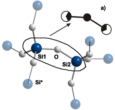
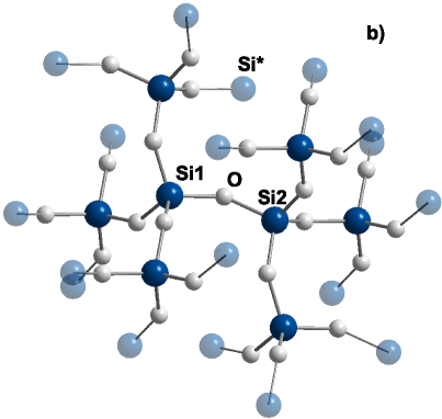
Figure 1: The first two quantum clusters, Si₂O₇ (a) and Si₈O₂₅ (b), used in our HF calculations. Point charges surrounding the clusters are not shown. Both silicon atoms (Si1 and Si2) and the oxygen atom of the central unit Si${}_{\frac{1}{4}}$OSi${}_{\frac{1}{4}}$ are indicated in each case. The elementary “brick” the whole system can be composed from is shown schematically in (a).

Fig. 2 shows the convergence of the HF electron density with the size of the cluster along the Si1-O direction. We carefully checked, by plotting the densities along other directions and by making 2D plots, that this direction is representative for assessing the convergence in this system. The deep minimum in the density at the oxygen atom is due to the pseudopotential method used. One can see that the difference between curves for the middle sized and the largest clusters is negligible. This suggests that the middle sized cluster Si₈O₂₅ is perfectly sufficient for our purposes and thus was used in all the calculations described below.

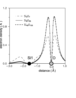
Figure 2: The HF electron densities for the three clusters are plotted along the Si1-O direction. The convergence is obvious: the curves for the middle sized and the largest clusters are indistinguishable.

As has been mentioned above, the elementary “brick” we can build the system from is the unit Si${}_{\frac{1}{4}}$OSi${}_{\frac{1}{4}}$ shown in the centre of each of the clusters in Fig.1 as a Si1-O-Si2 molecule. Each such unit should be assigned 8 electrons in total: 6 electrons come from the O atom and by 1 electron from each of the two Si atoms. Note that each Si atom contributes to four different units which contain this Si atom. This simple analysis allows us to suggest at least three possible choices (models) for the localisation regions:

1. Each unit Si${}_{\frac{1}{4}}$OSi${}_{\frac{1}{4}}$containing 8 electrons is considered as a single region; therefore, to obtain the corresponding four (double occupied) LMO’s, one has to choose all AO’s centred on the atoms Si1, Si2 and O in the centre of the cluster when applying any of the localising functionals discussed above. Note that all four LMO’s obtained using this partition method will be orthonormal as eigenvectors of the same secular problem (4).

2. Each pair of atoms Si1-O and Si2-O can be considered as a separate region, i.e. there will be two regions in total to describe every unit Si${}_{\frac{1}{4}}$OSi${}_{\frac{1}{4}}$; four electrons distributed over two (double occupied) LMO’s will be associated in this case with each of the two regions. Two LMO’s associated with either of the two regions will be mutually orthogonal; however, the LMO’s belonging to different regions will have a non-zero overlap.

3. Finally, each unit can be split into three different regions: (i) the first region, containing two electrons and described by a single LMO, is constructed to describe a covalent bond Si1-O; this can be achieved by enforcing localisation on $2p$ AO’s of the O atom and all AO’s of the Si1 atom; (ii) the second region is formed similarly to describe the Si2-O bond; (iii) finally, the remaining four electrons are attached to the third region which is localised predominantly on the O atom giving rise to two more (double occupied) LMO’s; in this case the $2s$ AO’s centred on the O atom can be used to inforce localisation. Thus, in this case there will be three sets of the LMO’s: two orthogonal LMO’s belonging to the O region and other two LMO’s belonging to the “bond” regions; the latter two LMO’s have a non-zero overlap with any other LMO.

For each choice of the localisation regions described above (which will be referred to as regions models hereafter), we can apply either of the three localisation methods of Section 2 to calculate the LMO’s using the obtained occupied canonical orbitals of the middle cluster. When solving the secular problem (4), the contributions of the boundary pseudoatoms Si* were removed from the canonical orbitals which then were renormalised. Using the obtained LMO’s, one should appropriately translate and rotate them in order to obtain all LMO’s comprising the whole primitive cell. (For instance, there will be six sets with four LMO’s in each in the primitive cell for model 1.) By applying lattice translations to all the LMO’s associated with the primitive cell, the whole infinite crystal is reproduced. It is then possible to calculate the total electron density $\rho(\mathbf{r)}$ of the whole crystal using Eq. (3). The necessary lattice summations are handled exactly by converting into the $\mathbf{k}$ space [24]. These calculations have been done for all nine cases (three localisation methods versus three choices of the localisation regions). The calculated $\rho(\mathbf{r)}$ matched exactly the original HF density in the central part of the cluster in all cases indicating that a very good degree of localisation was achieved in each case. As an example, a 2D contour plot of the total valence electron density in the plane of the molecule Si1-O-Si2 calculated using LMO’s obtained by method M in model 1 is shown in Fig. 3.

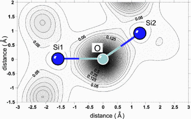
Figure 3: The total electron valence density $\rho(\mathbf{r})$ in the Si1-O-Si2 plane by combining the contributions of LMO’s (method M, model 1) across the infinite crystal. The density was calculated using the method [24] based on Eq. (3).

The cross-section of this plot corresponds to a solid line (the middle cluster) in Fig. 2. One can see that a considerable amount of the charge is concentrated around oxygen atoms.

The partial region densities, $\rho_{A}(\mathbf{r})=\sigma_{A}(\mathbf{r},\mathbf{r})$ (see Eq. (5)), corresponding to each of the regions and generated from the LMO’s calculated using method M, are shown in Fig. 4 as closed 3D surfaces of constant density. The value of the density is chosen in such a way so that 90% of the region electron charge be contained inside every surface. In the case of model 1 (the upper panel) only one density is shown; in the case of model 2 (the middle panel) two densities are shown simultaneously, while in the third case (model 3, the bottom panel), all three partial densities are presented. One can see that in the cases of models 2 and 3 the LMO’s belonging to neighbouring regions strongly overlap. As was mentioned before, the LMO’s belonging to different regions for these two models are not orthogonal. At the same time, the overall shapes of the density for each of the region models are very similar demonstrating a clear aggregation around the O atom in the middle of the Si${}_{\frac{1}{4}}$OSi${}_{\frac{1}{4}}$ unit in agreement with the total density shown in Fig. 3.

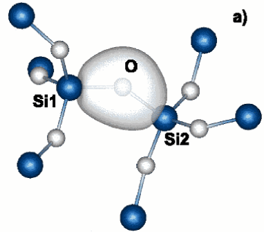
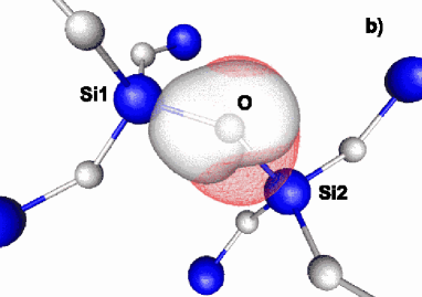
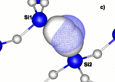
Figure 4: Constant partial density plots for three choices of localisation regions: (a) model 1, when the whole unit Si${}_{\frac{1}{4}}$OSi${}_{\frac{1}{4}}$ is associated with a single region; (b) model 2, when two regions Si1-O and Si2-O are identified and (c) model 3, when three regions, Si1-O, Si2-O and O, are identified. In every case the value of the density shown is chosen to enclose 90% of the total electron charge associated with the region. The localisation method M was used in each case.

A comparison of the LMO’s calculated using three localisation methods is presented in Fig. 5 for region model 1. In this figure, the partial densities $\rho_{A}(r)$ are shown in each case along the Si1-O direction through the Si${}_{\frac{1}{4}}$OSi${}_{\frac{1}{4}}$ unit. It is clear that the partial density obtained from LMO’s calculated using method M are found slightly more localised, whereas the localisation obtained using method P is slightly worse than given by the two others. Still, the difference between the densities is extremely small so that we can conclude at this point that all three techniques perform practically equally well (at least for the system under discussion).

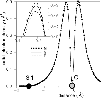
Figure 5: The partial electron density for region model 1 calculated using different localisation methods and plotted along the Si1-O direction.

The picture becomes more complicated, however, at least at the first sight, when the localisation criteria of Section 2.3 are applied in each of the nine cases as shown in Table 1. Three rows in this table correspond to the three different region models; in each case there are four LMO’s in total which are occupied by eight electrons of the elementary Si${}_{\frac{1}{4}}$OSi${}_{\frac{1}{4}}$ unit. The three columns in the Table correspond to the three different localisation methods used, and each of the localisation criteria is shown for every method.

The fist criterion (the localisation index $d_{a}$) is slightly above one in most cases, and is smaller than two in all nine cases. This means that the LMO’s are mostly localised on a single atom with some contribution coming from the nearest atoms. However, the maximum eigenvalues of the overlap matrix were found to be below two only for the region model 1 and localisation methods M and G; in the cases of models 2 and 3 eigenvalues around three were found indicating worse localisation. Finally, the gap between the eigenvalues of the secular problem of Eq. (4), $\Delta\lambda$, was found to be too small for the region models 2 and 3, whereas in the case of model 1 and for all three localisation methods the gap is considerable, especially for methods M and G. This means that the choice of the regions in models 2 and 3 is somewhat artificial which is not surprising because of a very strong overlap between LMO’s corresponding to the neighbouring regions in these two models.

It follows from this analysis that the model 1, in which the whole elementary unit Si${}_{\frac{1}{4}}$OSi${}_{\frac{1}{4}}$ is considered as one region, results in the best localisation of the LMO’s, especially if methods M and G are used.

		LMO	Method M			Method G			Method P
Model	Regions		$d_{a}$	$\max(\lambda(\mathbf{k}))$	$\Delta\lambda$	$d_{a}$	$\max(\lambda(\mathbf{k}))$	$\Delta\lambda$	$d_{a}$	$\max(\lambda(\mathbf{k}))$	$\Delta\lambda$
		1	1.18573			1.20741			1.22195
1	Si1-O-Si2	2	1.13868	1.71955	0.92527	1.15423	1.76597	0.77451	1.54019	2.08836	0.30218
		3	1.41971			1.44083			1.17747
		4	1.12914			1.13788			1.18254
	Si1-O	1	1.21753		0.00508	1.20624		0.00223	1.24733		0.00045
2		2	1.15569	2.97523		1.17676	2.92854		1.24529	3.07121
	Si2-O	1	1.20410		0.01659	1.18245		0.00736	1.24529		0.00108
		2	1.16580			1.19308			1.18726
	O	1	1.07793		0.06952	1.06777		0.04513	1.11378		0.00112
3		2	1.12734	3.43867		1.11958	3.43770		1.12776	3.98629
	Si1-O	1	1.21753		0.02072	1.20624		0.01363	1.24733		0.00433
	Si2-O	1	1.20410		0.00921	1.18245		0.00868	1.24529		0.00409

Table 1: Localisation criteria calculated for all region models and localisation methods.

In spite of subtle differences in the applied localisation criteria which seem to favour the model 1 and the methods M and G, we stress that very good localisation of the LMO’s was obtained in all cases. This conclusion is also supported by an observation that LMO’s generated within different models (choices of the regions) span the same Fock space. To make such a conclusion, we calculated the projection of the LMO’s of models 2 and 3 on the space spanned by the four orthogonal LMO’s obtained in model 1 and then subtracted the projection from the original orbitals. The calculated residual parts were found negligible in all cases. Note, that this conclusion is not obvious because each LMO depends on all AO’s of the entire cluster.

4 Conclusions

In this paper we have calculated strongly localised molecular orbitals (LMO’s) for the SiO₂ crystal ($\alpha$-quartz) using the method developed earlier [16]. The starting point for the choice of the localisation regions was an observation that the whole crystal can be reproduced by rotating and translating a single elementary unit Si${}_{\frac{1}{4}}$OSi${}_{\frac{1}{4}}$, containing an O atom and quarters of the two Si atoms which the O atom is directly connected to. Three localisation methods were applied and three models for choosing the localisation regions were tried in each case: (1) the whole unit was considered as one region; (2) the unit was split into two and (3) three regions. Although in all cases well localised orbitals were obtained, we find that the first choice of the localisation region in which the whole unit was chosen as a single region, is preferable.

The LMO’s produced in models 2 and 3 were found very close to a linear combination of the orthonormal LMO’s obtained within model 1. If taken from the nearest regions belonging to the same elementary unit, they appeared to have a significant overlap with each other. On the other hand, the LMO’s belonging to different units (in either of the models) do not overlap strongly which is confirmed by various localisation criteria applied in this work and by the corresponding plots of the partial densities.

Since our previous calculations reported in [16] were done for the extreme cases of ionic (MgO) and covalent (Si) bonding, it follows from the results of the present study that our method is also applicable to the crystals with intermediate types of chemical bonding.

Note that we did not consider in this study localisation method E [16] based on the energy minimisation of the structure element corresponding to the chosen region. This is because it was found in [16] that the orbitals obtained by this method for the Si crystal were not sufficiently localised.

Although the LMO’s reported in this work may be useful to characterise the chemical bonding in the given crystal, they are needed for the embedding method which is under development. Different possibilities in choosing localisation regions open up various ways in terminating the quantum cluster when considering, e.g. a point defect in the crystal bulk or an adsorbed species on the crystal surface. This variety of options may be extremely useful in applications to keep the size of the cluster as small as possible. If, for instance, one would like to terminate the cluster with Si atoms, then either of the region models can be used (model 1 would probably be more convenient as the orbitals within each region are orthonormal). However, if a termination with oxygens is required, then region models 2 or 3 may prove to be more useful. In practice, a combination of terminations may be preferable, when both Si and O atoms are used at the boundary. In those cases all three models for choosing localisation regions may be employed.

Acknowledgements

O.D. would like to acknowledge the financial support from the Leverhulme Trust (grant F/07134/S) which has made this work possible. We would also like to thank S. Hao for help in the VASP calculations.

References

- [1] J. Sauer and M. Sierka, J. Comp. Chem. 21, 1470 (2000).
- [2] R. B. Murphy, D. M. Philipp, and R. A. Freisner, J. Comp. Chem. 21, 1442 (2000).
- [3] L. N. Kantorovich, J. Phys. C: Solid State Phys. 21, 5041 (1988).
- [4] L. N. Kantorovich, J. Phys. C: Solid State Phys. 21, 5057 (1988).
- [5] T. Vreven and K. Morokuma, J. Comp. Chem. 21, 1419 (2000).
- [6] I. V. Abarenkov et al., Phys. Rev. B 56, 1743 (1997).
- [7] D. Bakowies and W. Thiel, J. Phys. Chem. 100, 10580 (1996).
- [8] R. J. Hall, S. A. Hinde, N. A. Burton, and I. H. Hillier, J. Comp. Chem. 21, 1433 (2000).
- [9] X. Assfeld and J.-L. Rivail, Chem. Phys. Letters 263, 100 (1996).
- [10] T. Bredow, Int. J. Quant. Chem. 75, 127 (1999).
- [11] P. V. Sushko, A. L. Shluger, and C. R. A. Catlow, Surf. Science 450, 153 (2000).
- [12] V. Nasluzov et al., J.Chem.Phys. 115, 8157 (2001).
- [13] L. S. Seijo and Z. Barandiaran, Intern. J. Quant. Chem. 60, 617 (1996).
- [14] D. Erbetta, D. Ricci, and G. Pacchioni, J. Chem. Phys. 113, 10744 (2000).
- [15] V. Sulimov, P. Sushko, A. Edwards, A. Shluger, and A. Stoneham, Phys. Rev. B 66, 024108 (2002).
- [16] O. Danyliv and L. Kantorovich, Phys. Rev. B (2004), submitted (physics/040110).
- [17] R. Dovesi et al., CRYSTAL98 User’s Manual (University of Torino, Torino, 1998).
- [18] R. McWeeny, Methods of Molecular Quantum Mechanics (Academic Press, London, 1992).
- [19] I. Mayer, J. Phys.: Chem. 100, 6249 (1996).
- [20] R. S. Mulliken, J. Chem. Phys. 49, 497 (1949).
- [21] V. Magnasco and A. Perico, J. Chem. Phys. 47, 971 (1967).
- [22] J. Pipek and P. G. Mezey, J. Chem. Phys. 90, 4916 (1989).
- [23] K. Roby, Mol. Phys. 27, 81 (1974).
- [24] O. Danyliv and L. Kantorovich, J. Phys.: Condens. Matter 16, 2575 (2004).
- [25] J. L. Whitten and T. A. Pakkanen, Phys. Rev. B 21, 4357 (1980).
- [26] R. W. G. Wyckoff, Crystal structures, 2nd ed. (Wiley, New York, 1963).
- [27] L. Kantorovich, Quantum theory of the solid state: an introduction.Fundamental Theories of Physics (Kluwer Academic Publishers, Dordrecht, 2004).
- [28] G. Kresse and J. Furthmüller, Comp. Mat. Sci. 6, 15 (1996).
- [29] G. Kresse and J. Furthmüller, Phys. Rev. B 54, 11169 (1996).
- [30] G. Kresse and J. Hafner, J. Phys.: Condens. Matter 6, 8245 (1994).
- [31] C. Melius and W. Goddard III, Phys. Rev. A 10, 1528 (1974).
- [32] M. F. Guest et al., GAMESS-UK, a package of ab initio programs, , nrcc software catalog, vol. 1, program no. qg01 ed., 1980.