Possibility of an ultra-precise optical clock using the $6\,^{1}\!S_{0}\rightarrow 6\,^{3}\!P^{o}_{0}$ transition in ^171,173Yb atoms held in an optical lattice

Abstract

We report calculations designed to assess the ultimate precision of an atomic clock based on the 578 nm $6\,^{1}\!S_{0}\rightarrow 6\,^{3}\!P^{o}_{0}$ transition in Yb atoms confined in an optical lattice trap. We find that this transition has a natural linewidth less than 10 mHz in the odd Yb isotopes, caused by hyperfine coupling. The shift in this transition due to the trapping light acting through the lowest order AC polarizability is found to become zero at the magic trap wavelength of about 752 nm. The effects of Rayleigh scattering, higher-order polarizabilities, vector polarizability, and hyperfine induced electronic magnetic moments can all be held below a mHz (about a part in $10^{18}$), except in the case of the hyperpolarizability larger shifts due to nearly resonant terms cannot be ruled out without an accurate measurement of the magic wavelength.

Optical atomic clocks offer new opportunities for creating improved time standards as well as looking for changes in fundamental constants over time, measuring gravitational red shifts, and timing pulsars. Compared with microwave atomic clocks, optical clocks have the intrinsic advantage that optical transitions have a much higher frequency and potentially much higher line-Q than microwave transitions. Moreover, optical frequency comb techniques Stenger et al. (2002) now permit different optical frequencies to be compared with each other at the $10^{-17}$ level or better, and to be linked to microwave clocks as well. Optical transitions in alkaline earth atoms offer remarkable possibilities for clocks. In addition to the relatively sharp ${}^{1}\!S_{0}\rightarrow\ ^{3}\!P_{1}^{o}$ intercombination line already in use Diddams et al. (2001), there occurs the much sharper ${}^{1}\!S_{0}\rightarrow\ ^{3}\!P_{0}^{o}$ line in odd isotopes. This one-photon transition is forbidden in even isotopes, but in odd isotopes acquires a weak E1 amplitude induced by the internal hyperfine coupling of the nuclear spin. Doppler and recoil shifts can be virtually eliminated by confining very cold atoms in an optical lattice trap. This lattice will be Stark-free if it is produced by laser beams tuned to the magic frequency where the ground and excited states undergo the same light shift, leaving the clock transition unshifted and relatively insensitive to the laser polarization.

Katori Katori (2002) has pointed out these advantages for ⁸⁷Sr, and the $5\,^{1}\!S_{0}\rightarrow 5\,^{3}\!P_{0}^{o}$ transition in this isotope has recently been observed Courtillot et al. (2003). Also, Sr atoms have been held in an optical lattice at the laser wavelength appropriate for a Stark-free $5\,^{1}\!S_{0}\rightarrow 5\,^{3}\!P_{1}^{o}$ transition, and this transition has been observed free of Doppler and recoil shifts Ido and Katori (2003). The magic frequency for the Sr clock has been evaluated recently in Ref. Katori et al. (2003) and it has been measured in Ref. Takamoto and Katori (2003). In Ref. Katori et al. (2003) an estimate of systematic uncertainties for Sr also has been carried out.

Ytterbium has two stable odd isotopes, ¹⁷¹Yb and ¹⁷³Yb, which also appear to be excellent candidates for an atomic standard, using the $6\,^{1}\!S_{0}\rightarrow 6\,^{3}\!P_{0}^{o}$ transition at the convenient wavelength 578 nm. The atoms are readily trapped into a MOT operating on either the strong $6\,^{1}\!S_{0}\rightarrow 6\,^{1}\!P_{1}^{o}$ line or the $6\,^{1}\!S_{0}\rightarrow 6\,^{3}\!P_{1}^{o}$ intercombination line and in the latter case have been cooled to $\mu$K temperatures by Sisyphus cooling Maruyama et al. (2003). Also, these isotopes have been successfully confined in an optical dipole trap Honda et al. (2002). In this paper we present a calculation of the natural linewidth of the clock transition, which turns out to be less than 10 mHz, and also a calculation of the Stark-free wavelength of an optical lattice trap for the clock transition. This wavelength turns out to be about 752 nm, reachable with adequate power by a tunable Ti:Sa laser. We also estimate the size of the polarizability due to higher magnetic dipole and electric quadrupole optical moments. In addition, we estimate the Rayleigh and Raman scattering rates in the optical lattice which can limit the coherence lifetime of the clock transition. Finally, we compute the small but important hyperfine-induced Zeeman shift in the excited state and the vector light shift which can cause a small Stark-shift dependence on the polarization of the trapping light.

Our results indicate that a light intensity of 10 kW/cm² would create a convenient trap depth of 15 $\mu$K at the magic wavelength, while perturbations to the clock frequency could be held below the mHz level ($10^{-18}$ relative shift) – with one possible exception. Larger shifts due to accidental near resonances in the hyperpolarizability cannot be ruled out without an accurate measurement of the magic wavelength.

All the calculations reported in this paper have been carried out using the relativistic many-body code described in Refs. Dzuba et al. (1996, 1998); Kozlov and Porsev (1999). The employed formalism is a combination of configuration-interaction method in the valence space with many-body perturbation theory for core-polarization effects. The effective core-polarization (self-energy) operator is adjusted so that the experimental energy levels are well reproduced. In addition, the dressing of the external electromagnetic field (so-called core shielding) is included in the framework of the random-phase approximation. In the following we refer to this many-body method as CI+MBPT. For Yb, the CI+MBPT method has an accuracy of a few per cent for electric dipole matrix elements and magnetic-dipole hyperfine constants Porsev et al. (1999a, b). Unless specified otherwise, we use atomic units ($|e|=\hbar=m_{e}\equiv 1$) throughout the paper.

In the proposed design, the Yb atoms are confined to sites of an optical lattice (formed by a standing-wave laser field of frequency $\omega$ and amplitude of electric field $\mathcal{E}_{0}$). To the leading order in intensity and the fine-structure constant, the laser field shifts the clock transition frequency $\omega_{0}$ by

$$\delta\omega_{0}(\omega)=-\left\{\alpha_{6\,^{3}\!P_{0}^{o}}^{E1}\left(\omega\right)-\alpha_{6\,^{1}\!S_{0}}^{E1}\left(\omega\right)\right\}\left(\mathcal{E}_{0}/2\right)^{2}\,,$$ (1)

where $\alpha_{X}^{E1}\left(\omega\right)$ is an a.c. electric-dipole polarizability of level $X$

$$\alpha_{X}^{{}_{E1}}\left(\omega\right)=2\,\sum_{Y}\frac{E_{Y}-E_{X}}{\left(E_{Y}-E_{X}\right)^{2}-\omega^{2}}\left|\langle X|D_{z}|Y\rangle\right|^{2}\,.$$ (2)

We have carried out the calculations of the E1 a.c. polarizability using the CI+MBPT method. We summed over the intermediate states in Eq. (2) using the Dalgarno-Lewis-Sternheimer method Dalgarno and Lewis (1955). The results of the calculations for both $6\,^{1}\!S_{0}$ and $6\,^{3}\!P_{0}^{o}$ states are shown in Fig. 1. The two dynamic polarizabilities intersect at $\omega^{\ast}=0.0606$ a.u. At this “magic” frequency the lowest-order differential light-shift, Eq. (1), vanishes. It is worth noting that at $\omega^{\ast}$ the sum (2) for the ground state is dominated by the $6s6p\,^{1}\!P_{1}^{o}$ state and for the $6\,^{3}\!P_{0}^{o}$ level by the $6s7s\,^{3}S_{1}$ state.

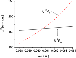
Figure 1: Electric dipole a.c. polarizabilities for $6\,^{1}\!S_{0}$ (solid line) and $6\,^{3}\!P_{0}$ (dashed line) states of Yb. The polarizabilities are shown as a function of laser frequency $\omega$.

In general, for a linear laser polarization the second-order light shift of level $X$ can be represented as a sum over $2^{J}$-pole polarizabilities $\alpha_{X}^{\left(J\lambda\right)}$ ($\lambda$ distinguishes between electric, $\lambda=1$, and magnetic, $\lambda=0$, multipoles)

$$\delta E_{X}=-\frac{\mathcal{E}_{0}^{2}}{4}\sum_{J\lambda}\alpha_{X}^{\left(J\lambda\right)}\left(\omega\right)\,.$$ (3)

When the total angular momentum of the level $X$ is equal to zero these a.c. polarizabilities are expressed as

$$\alpha_{X}^{\left(J\lambda\right)}\left(\omega\right) = \frac{J+1}{J}\frac{2J+1}{\left[\left(2J+1\right)!!\right]^{2}}\left(\alpha\omega\right)^{2J-2}\times$$

$$\sum_{Y}\left\{\frac{(E_{Y}-E_{X})\left|\langle Y||Q^{\left(J\lambda\right)}||X\rangle\right|^{2}}{\left(E_{Y}-E_{X}\right)^{2}-\omega^{2}}\right\}\,,$$

with $Q^{\left(J\lambda\right)}$ being relevant multipole operators Johnson et al. (1995). Typically, the E1 polarizability (2) overwhelms this sum. Compared to the E1 contribution, the higher-order multipole polarizabilities are suppressed by a factor of $(\alpha\omega)^{2J-2}$ for EJ and by a factor of $\alpha^{2}(\alpha\omega)^{2J-2}$ for MJ multipoles. We verified that at the magic frequency there are no resonant contributions for the next-order E2 and M1 polarizabilities and we expect $\alpha^{(E2,M1)}\lesssim 10^{-6}\alpha^{(E1)}$, similar to the case of Sr  Katori et al. (2003). At the same time we notice that a core-excited state $4f^{13}(^{2}\!F_{7/2}^{\circ})5d_{5/2}6s^{2}$ $J=5$ may become resonant with an excitation from the $6\,^{3}\!P_{0}^{o}$ level. The relevant $M5$ polarizability is highly suppressed, and we anticipate that the magic frequency will be only slightly shifted by the presence of this state.

Higher-order correction to the differential frequency shift, Eq.(1), arises due to terms quartic in the field strength $\mathcal{E}_{0}$. This fourth-order contribution is expressed in terms of a.c. hyperpolarizability $\gamma(\omega)$. The expression for $\gamma(\omega)$ Manakov et al. (1986) has a complicated energy denominator structure exhibiting both single– and two–photon resonances. While for the ground state there are no such resonances, for the $6\,^{3}\,P_{0}^{o}$ a two-photon resonance may occur for $6s8p\,^{1}\!P_{1}^{o}$ and $6s8p\,^{3}\!P_{J}^{o}$ intermediate states. Due to theoretical errors in calculations of the magic frequency we can not reliably predict if the two-photon resonances would occur. Since the resonance contributions may dominate $\gamma(\omega)$, we can not provide a reliable estimate of the fourth-order frequency shift. The estimate may be carried out as soon as the magic frequency is measured with sufficient resolution. As a possible indication of the effect on the clock frequency, we notice that for Sr Katori et al. (2003) the resulting correction to the energy levels was a few mHz at a trapping laser intensity of 10 kW/cm². This systematic uncertainty can be controlled by studying the dependence of the level shift on the laser intensity Ido and Katori (2003).

The $6\,^{3}\!P_{0}^{o}$ state decays due to an admixture from $J=1$ states caused by the hyperfine interaction. In this paper we restrict our attention to the hyperfine interaction due to the nuclear magnetic moment $\mathbf{\mu}$. We write this interaction as $H_{\mathrm{hfs}}=\left(\mathbf{\mu}/\mu_{N}\cdot\mathbf{T}_{e}^{\left(1\right)}\right)$, where tensor $\mathbf{T}_{e}^{\left(1\right)}$ acts on the electronic coordinates and $\mu_{N}$ is the nuclear magneton. We employ the following nuclear parameters: for ¹⁷¹Yb, the nuclear spin $I=1/2$ and magnetic moment $\mu=0.4919\,\mu_{N}$, and for ¹⁷³Yb, $I=5/2$ and $\mu=-0.6776\,\mu_{N}$. Using first-order perturbation theory, the HFS-induced transition rate is given by

$$A_{\mathrm{hfs}}\left(6\,^{3}\!P_{0}^{o}\right)=\frac{4\alpha^{3}}{27}\frac{\left(I+1\right)}{I}\left(\mu/\mu_{N}\right)^{2}~{}\omega_{0}^{3}~{}\left|S\right|^{2}\,,$$ (4)

where the sum $S$ is defined as

$$S=\sum_{\gamma^{\prime}}\frac{\langle 6\,^{1}\!S_{0}||D||\gamma^{\prime}\rangle\,\langle\gamma^{\prime}||\mathcal{T}_{e}^{\left(1\right)}||6\,^{3}\!P_{0}^{o}\rangle}{E\left(\gamma^{\prime}\right)-E\left(6\,^{3}\!P_{0}^{o}\right)}\,$$ (5)

and $\omega_{0}=E\left(6\,^{3}\!P_{0}^{o}\right)-E\left(6^{1}S_{0}\right)$.

To estimate the rate we restricted the summation over intermediate states to the nearest-energy $6\,^{1}\!P_{1}^{o}$ and $6\,^{3}\!P_{1}^{o}$ states. Using the CI+MBPT method we computed HFS couplings, $\langle 6^{3}\!P_{0}^{o}||\mathcal{T}_{e}^{\left(1\right)}||6\,^{3}\!P_{1}^{o}\rangle=-6685\,\mathrm{MHz}$ and $\langle 6\ ^{3}\!P_{0}^{o}||\mathcal{T}^{\left(1\right)}||6\,^{1}\!P_{1}^{o}\rangle=4019\,\mathrm{MHz}$ and we inferred the values of dipole matrix elements from lifetime measurements Bowers et al. (1996); Takahashi et al. (2003). The resulting HFS-induced lifetimes of the $6\,^{3}\!P_{0}^{o}$ level are 20 and 23 seconds for ¹⁷¹Yb and ¹⁷³Yb isotopes respectively.

A coherence of atomic states may be lost due to scattering of laser photons (Rayleigh and Raman processes Berestetskii et al. (1982)). These are second order processes. In particular, the Rayleigh (heating) rate for both $6\,^{3}\!P_{0}^{o}$ and the ground states may be expressed in terms of a.c. polarizability

$$\gamma_{h}=\alpha^{4}\,\frac{8\pi}{3}\,(\omega^{\ast})^{3}\,\left[\alpha^{E1}\left(\omega^{\ast}\right)\right]^{2}I_{L}\,,$$

where $I_{L}$ is the intensity of laser. At the magic frequency $\omega^{\ast}$ the values of a.c. polarizability for both states are equal to 160 a.u. (see Fig. 1). For a laser intensity of 10 kW/cm², the resulting rate is in the order of $10^{-3}$ sec^-1. As to the Raman rates, there are no Raman transitions originating from the ground state. The final states for transitions from the $6\,^{3}\!P_{0}^{o}$ are the $J=1,2$ sublevels of the same $6\,^{3}\!P_{J}^{o}$ fine-structure multiplet. We estimate this rate by approximating the relevant second-order sum with the dominant contribution from the $6s7s\,^{3}\!S_{1}$ intermediate state. The resulting Raman scattering rate is also in the order of $10^{-3}$ sec^-1 for 10 kW/cm² laser.

The total magnetic moment of the Yb atom is composed of the nuclear and electronic magnetic moments. Disregarding shielding of externally applied magnetic fields by atomic electrons, the $g$-factor due to the nuclear moment is given by $\delta g_{\mathrm{nuc}}=-(1/m_{p})(\mu/\mu_{N})/I$, where $m_{p}$ is the proton mass. The numerical values of $\delta g_{\mathrm{nuc}}$ are $-5.4\times 10^{-4}$ for ¹⁷¹Yb and $1.48\times 10^{-4}$ for ¹⁷³Yb. The electronic magnetic moment of the $6\,^{3}\!P_{0}^{o}$ state arises due to mixing of levels caused by the hyperfine interaction, i.e., the same mechanism that causes the $6\,^{3}\!P_{0}^{o}$ state to decay radiatively. This correction may be expressed as

$$\delta g_{\mathrm{hfs}}\approx\frac{\sqrt{8}}{3}\;\frac{1}{I}\frac{\mu}{\mu_{N}}\frac{\langle 6\,^{3}\!P_{1}^{o}||\mathcal{T}_{e}^{\left(1\right)}||6\,^{3}\!P_{0}^{o}\rangle}{E\left(6\,^{3}\!P_{1}^{o}\right)-E\left(6\,^{3}\!P_{0}^{o}\right)}\,.$$

The computed values of the $\delta g_{\mathrm{hfs}}$ correction are $2.9~{}\times 10^{-4}$ for ¹⁷¹Yb and $-8.1\times 10^{-5}$ for ¹⁷³Yb, which imply that mHz shifts would be produced by $\mu$G magnetic fields. Fields can readily be calibrated and stabilized to this level using magnetic shielding.

The hyperfine interaction also induces residual vector (axial) $\alpha_{\gamma F}^{A}\left(\omega\right)$ and tensor $\alpha_{\gamma F}^{T}\left(\omega\right)$ a.c. polarizabilities. For $J=0$ levels there is no tensor contribution for the ¹⁷¹Yb isotope ($I=1/2$) and it can be shown that for the ¹⁷³Yb ($I=5/2$) it vanishes when the HFS interaction is restricted to the dominant magnetic-dipole term. For a non-zero degree of circular polarization $\mathcal{A}$, the relevant correction to the light shift of level $\gamma F$ is

$$\delta E_{\gamma F}^{(A)}=-\frac{M}{2F}\mathcal{A}~{}\alpha_{\gamma F}^{A}\left(\omega\right)\left(\frac{1}{2}\mathcal{E}_{0}\right)^{2}\,,$$ (6)

where for $J=0$, $F=I$ and $M$ is the magnetic quantum number. Using third-order perturbation theory and a formalism of quasi-energy states Manakov et al. (1986) we arrived at an expression for $\alpha_{\gamma F}^{A}\left(\omega\right)$ which contains two dipole and one hyperfine operator in various orderings and double summations over intermediate states. Analyzing these expressions, we find that the vector polarizability of the $6^{3}\!P_{0}^{o}$ state is much larger than that for the ground state, as in the case of Sr  Katori et al. (2003). For Sr, Katori et al. (2003) estimated the vector polarizability by adding HFS correction to the energy levels of intermediate states in Eq. (2). Our analysis is more complete and we find that the dominant effect is not due to corrections to the energy levels, but it is rather due to perturbation of the $6^{3}\!P^{o}_{0}$ state by the HFS operator. The resulting values of $\alpha_{6^{3}\!P^{o}_{0}}^{A}\left(\omega^{\ast}\right)$ are $-0.10$ a.u. for ¹⁷¹Yb and $0.075$ a.u. for ¹⁷³Yb. Using these values in the above equation, we find that holding $\mathcal{A}$ to $<10^{-6}$ with fields of 10 kW/cm² would keep shifts in the clock frequency below the mHz level. This requirement on optical polarization is not an extreme one, and in the special case of a 1D optical lattice could be relaxed significantly by orienting the quantization axis (defined by the external magnetic field) perpendicular to the trap axis.

In conclusion, we have analyzed the possibility of creating a highly precise optical clock operating on the $6\,^{1}\!S_{0}\rightarrow 6\,^{3}\!P_{0}^{o}$ transition in odd isotopes of atomic Yb. According to our calculations, the natural linewidth is about 10 mHz, and the magic wavelength for producing zero Stark shift of this transition in an optical lattice trap is about 752 nm. We have examined possible sources of shifts and broadening due to both the optical trapping fields and any magnetic fields, and find they should not perturb the clock above the $10^{-18}$ level, except for possible larger near-resonant terms in the hyperpolarizability. An accurate measurement of the magic wavelength will be needed to settle this last question.

This work was partially supported by the National Science Foundation, grants PHY 0099535 and PHY 0099419. The work of S.G.P. was partially supported by the Russian Foundation for Basic Research under grant No 02-02-16837-a.

References

- Stenger et al. (2002) J. Stenger, H. Schnatz, C. Tamm, and H. R. Telle, Phys. Rev. Lett. 88, 073601/1 (2002).
- Diddams et al. (2001) S. A. Diddams, T. Udem, J. C. Bergquist, E. A. Curtis, R. E. Drullinger, L. Hollberg, W. M. Itano, W. D. Lee, C. W. Oates, K. R. Vogel, et al., Science 293, 825 (2001).
- Katori (2002) H. Katori, in Proc. 6th Symposium Frequency Standards and Metrology, edited by P. Gill (World Scientific, Singapore, 2002), pp. 323–330.
- Courtillot et al. (2003) I. Courtillot, A. Quessada, R. P. Kovacich, A. Brusch, D. Kolker, J.-J. Zondy, G. D. Rovera, and P. Lemonde (2003), http://arXiv.org/abs/physics/0303023.
- Ido and Katori (2003) T. Ido and H. Katori, Phys. Rev. Lett. 91, 053001/1 (2003).
- Katori et al. (2003) H. Katori, M. Takamoto, V. G. Pal’chikov, and V. D. Ovsiannikov, Phys. Rev. Lett. (in press) (2003), physics/0309043.
- Takamoto and Katori (2003) M. Takamoto and H. Katori, submitted to Phys. Rev. Lett. (2003), physics/0309044.
- Maruyama et al. (2003) R. Maruyama, R. Wynar, M. V. Romalis, A. Andalkar, M. D. Swallows, C. E. Pearson, and E. N. Fortson, Phys. Rev. A 68, 11403/1 (2003).
- Honda et al. (2002) K. Honda, Y. Takasu, T. Kuwamoto, M. Kumakura, Y. Takahashi, and T. Yabuzaki, Phys. Rev. A 66, 021401/1 (2002).
- Dzuba et al. (1996) V. A. Dzuba, V. V. Flambaum, and M. G. Kozlov, Phys. Rev. A 54, 3948 (1996).
- Dzuba et al. (1998) V. A. Dzuba, M. G. Kozlov, S. G. Porsev, and V. V. Flambaum, Zh. Eksp. Teor. Fiz. 114, 1636 (1998), [Sov. Phys.–JETP 87 885, (1998)].
- Kozlov and Porsev (1999) M. G. Kozlov and S. G. Porsev, Eur. Phys. J. D 5, 59 (1999).
- Porsev et al. (1999a) S. G. Porsev, Yu. G. Rakhlina, and M. G. Kozlov, Phys. Rev. A 60, 2781 (1999a).
- Porsev et al. (1999b) S. G. Porsev, Yu. G. Rakhlina, and M. G. Kozlov, J. Phys. B 32, 1113 (1999b).
- Dalgarno and Lewis (1955) A. Dalgarno and J. T. Lewis, Proc. Roy. Soc. 223, 70 (1955).
- Johnson et al. (1995) W. R. Johnson, D. R. Plante, and J. Sapirstein, Adv. At. Mol. Phys. 35, 255 (1995).
- Manakov et al. (1986) N. L. Manakov, V. D. Ovsiannikov, and L. P. Rapoport, Phys. Rep. 141, 319 (1986).
- Bowers et al. (1996) C. J. Bowers, D. Budker, E. D. Commins, D. DeMille, S. J. Freedman, A.-T. Nguyen, S.-Q. Shang, and M. Zolotorev, Phys. Rev. A 53, 3103 (1996), and references therein.
- Takahashi et al. (2003) Y. Takahashi, Y. Takasu, K. Komori, K. Honda, M. Kumakura, and T. Yabuzaki, in Proc. of XVIII International Conference on Atomic Physics, edited by H. R. Sadeghpour, D. E. Pritchard, and E. J. Heller (World Scientific, Singapore, 2003), p. 83.
- Berestetskii et al. (1982) V. B. Berestetskii, E. M. Lifshitz, and L. P. Pitaevskii, eds., Quantum Electrodynamics (Pergamon Press, Oxford, 1982), 2nd ed.