Experimental observation and characterization of the magnetorotational instability

Abstract

Differential rotation occurs in conducting flows in accretion disks and planetary cores. In such systems, the magnetorotational instability can arise from coupling Lorentz and centrifugal forces to cause large radial angular momentum fluxes. We present the first experimental observation of the magnetorotational instability. Our system consists of liquid sodium between differentially rotating spheres, with an imposed coaxial magnetic field. We characterize the observed patterns, dynamics and torque increases, and establish that this instability can occur from a hydrodynamic turbulent background.

Diverse astrophysical and planetary phenomena involve the close interplay of rotation and magnetic field generation. There is theoretical and computational evidence for a magnetorotational instability balbus 1991 ; balbus 1998 where magnetic fields destabilize differential rotation in electrically conducting flows velikhov ; chandra 1960 ; chandra 1961 . This instability is conceptually related to centrifugal instabilities such as the development of Taylor vortices, but the addition of Lorentz forces causes flows to be unstable even when centrifugally stable. An excellent description of the underlying process is given in two reviewsbalbus 1998 ; bal2003 . The instability leads to radial outflow of angular momentum, which in an astrophysical context implies the enhancement of the rate of inward matter flow pringle . It also leads to a type of magnetohydrodynamic turbulence, different from hydrodynamic turbulence by the forces in balance. The nature of and transition to magnetohydrodynamic turbulence is of much recent interest moresco ; krasnov ; ponty . The magnetorotational instability is thought to affect differentially rotating stars and planetary interiors balbus 1994 ; kitcha , and the dynamics of accretion disks in protostellar systems and around compact objects such as black holes begelman . In a geophysical or planetary context, the magnetorotational instability could serve as a mechanism for initial field growth leading to dynamo states requiring a finite amplitude initiation.

All our current understanding and appreciation of the magnetorotational instability derives from theory and numerical simulation balbus 1991 ; balbus 1998 ; hawley . Until now, there have been no direct observations of these phenomena in nature or the laboratory, although the suppression of centrifugal instabilities has been documented donnelly . In nature, the development of this instability occurs in contexts considerably more complicated than can be simulated, a primary problem being the possible presence of small scale hydrodynamic turbulence. A central issue we address is the growth of the magnetorotational instability within turbulent flows, which are unavoidable in experimental liquid metal flows in the proper parameter regime.

The experimental device (see Fig. 1) consists of sodium note1 flowing between a rotating inner sphere (radius $a=0.050$ m), and a stationary outer sphere. The inner sphere is made of high conductivity copper, mounted on a $0.0125$ m radius rotating non-magnetic stainless steel shaft which extends along the axis of rotation. The inner sphere rotates between $2.5$ to $50$ revolutions per second ($=\Omega_{o}/2\pi$). The $0.010$ m thick outer stationary vessel is a non-magnetic stainless steel shell (radius $b=0.15$ m). Due to its poor electrical conductivity, the outer vessel is relatively passive in the magnetic field dynamics peffley . An external magnetic field, from $B_{o}=0$ to $0.2$ T, is applied co-axially using a pair of electromagnets. We observe the induced fields using an array of $30$ external Hall probes note2 and the velocity using ultrasound Doppler velocimetry takeda ; note3 . The high electrical conductivity of sodium, the highest of any liquid davidson , allows significant interactions between the fluid flow and the currents causing induced magnetic fields, and allows an approach toward geophysically realistic parameters.

In addition to the radius ratio $a/b$, three important dimensionless numbers characterize our experiment. The magnetic Prandtl number, $P_{m}=\nu/\eta=8.8\times 10^{-6}$, is the ratio of kinematic viscosity $\nu$ to magnetic diffusivity $\eta$. A small value of $P_{m}$ is typical of liquid metals, planetary interiors and other natural systems, but distinguishes them from matter in accretion flows, for which $P_{m}\sim 1$. The Lundquist number, $S=B_{o}b/\eta(\rho\mu)^{1/2}$ (where $\rho$ is the density and $\mu$ the magnetic permeability), is the ratio of the Alfvén frequency to the resistive decay rate. For $S\sim 1$, system-size magnetic field oscillations within the sodium damp in about one period; shorter wavelengths are damped more strongly. The magnetic Reynolds number, $R_{m}=\Omega_{o}ab/\eta$, characterizes the ability of the fluid motions to create induced magnetic fields. Our experiments sisan access the relatively little-explored regime of parameter space $0<S<10$ and $0<R_{m}<25$. Another important (but dependent) parameter is the Reynolds number, $Re=R_{m}/P_{m}$. Because of the smallness of $P_{m}$, the Reynolds numbers for our experiments are large (varying between $1.7\times 10^{5}$ and $3.4\times 10^{6}$), implying well-developed hydrodynamic turbulence.

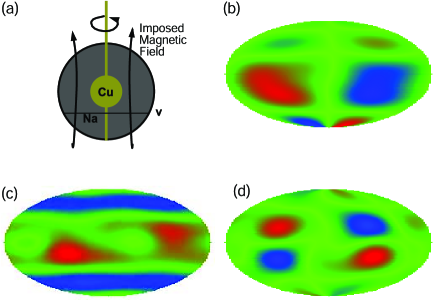
Figure 1: The spherical apparatus and characteristic induced magnetic field instability patterns. The device (a) consists of a thin stainless spherical outer vessel, a rotating inner copper sphere, and liquid sodium in between. The line adjacent to v indicates the location of the velocity measurements. The resulting dynamics change character under the influence of an externally applied magnetic field coaxial with the rotation. As the external field increases, one sees states dominated by (b) a rotating odd pattern with azimuthal wavenumber $m=1$ (O1) at $R_{m}=26$ ($50$ Hz), $S=4.19$ ($84.6$ mT), (c) an even $m=0$ pattern (E0) at $R_{m}=10.4$ ($20$ Hz), $S=4.37$ ($88.1$ mT), and (d) a rotating $m=1$ even pattern (E1) at $R_{m}=10.4$ ($20$ Hz), $S=7.08$ ($14.29$ mT). Red and blue indicate outward and inward radial (cylindrical) induced magnetic field, and green indicates the null values, in an equal area projection of the induced magnetic field just outside the outer sphere.

With no applied magnetic field (our base state), we have examined the mean flow along a chord perpendicular to the axis of rotation. It has a profile with a velocity exponent $\zeta=\partial\log\Omega(r)/\partial\log r$ in the range $\zeta\sim-1.4$ to $-1.6$ except in thin boundary layers near the walls (see Fig. 2). Here, $\Omega(r)$ is the rotation rate at a cylindrical radius $r$, and would satisfy $\Omega(r)\sim r^{\zeta}$ were $\zeta$ constant. For astrophysical rotation profiles governed by Kepler’s laws, $\zeta=-3/2$; that is, $\Omega^{2}r^{3}$ is constant. According to the hydrodynamic Rayleigh criterion, flows are linearly stable for $\zeta>-2$. Nevertheless, we observe $10-20\%$ turbulent velocity fluctuations in the base state, likely generated in the boundary layers, which will be fully described elsewhere. Smaller turbulent fluctuations are also observed in the magnetic field in the base state, due to interactions between the fluid turbulence and the Earth s relatively weak field, which is always present in the laboratory. Profiles with $\zeta<0$ are predicted to be magnetorotationally unstable, assuming a laminar base state. Precise stability boundaries have been calculated for liquid metals ($P_{m}\sim 10^{-6}$) in a cylindrical geometry ji ; goodman and for $P_{m}\sim 1$ flows in spherical geometry kitcha . Aside from a simple rescaling with $P_{m}$, the theoretical predictions are essentially identical: application of an axial magnetic field of strength sufficient to overcome resistivity will destabilize long-wavelength magnetorotationally driven oscillations.

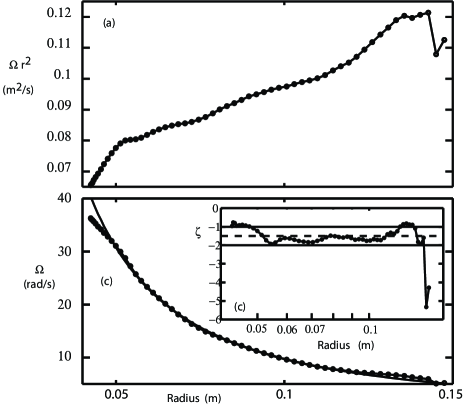
Figure 2: The zero field angular momentum and rotation rate profiles for $\Omega_{o}/2\pi=30$ Hz ($R_{m}=16$). From ultrasound velocimetry measurements, the rising mean angular momentum density (a) shows the system is stable to centrifugal instabilities except for thin boundary layers. The rotation curve (b) decreases with cylindrical radial distance from the center, a necessary condition for the base state to be unstable to the magnetorotational instability. The smooth curve is a Keplerian profile for comparison. The inset (c) shows the velocity exponent $\zeta$ with the Keplerian value $\zeta=-3/2$ indicated by a dashed line.

Our primary observation is that for fixed rotation rate of the inner sphere, above some threshold external magnetic field $B_{c}$, we observe spontaneous excitation of oscillating magnetic and velocity fields (Fig. 3). These take the form of a rotating pattern with azimuthal wavenumber $m=1$ (see Fig. 1b). At instability onset the applied torque increases (see Fig. 4), as increased amounts of angular momentum are carried from the inner sphere to the fixed outer sphere. These observations are evidence of the destabilization of the magnetorotational instability.

The fields and flows consist of toroidal and poloidal components bullard . The azimuthal mode numbers $m$ and the parity with respect to reflection through the origin characterize these components. The primary observed magnetic field instability (Fig. 4) is dominated by an $m=1$ poloidal perturbation that has odd parity. A toroidal magnetic field disturbance is also likely, but our Hall array, being outside the sodium, can only measure poloidal components. We denote the poloidal modes with the notation E$m$ (azimuthal wavenumber $m$ with even parity) and O$m$ (azimuthal wavenumber $m$ with odd parity). After our initial O1 instability, as the external magnetic field strength is further increased, a number of other modes appear. These include saturated states dominated by E0 (Fig. 1c), E1 (Fig. 1d), O2, and E2. For applied fields many times $B_{c}$, the modes often show aperiodic changes in pattern, rather than simple precession. By varying the rotation rate and external field independently, we have navigated the ($R_{m}$,$S$) parameter plane and determined the regions where these other modes dominate (Fig. 5).

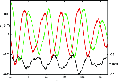
Figure 3: Coupled fluctuations in the velocity and magnetic fields. Here the amplitude of the induced field for the two Gauss modes O1 (top curves) and the amplitude of a velocity component (lower black curve) below the outer sphere substantiate that Lorentz forces are key to this instability. These data were taken at $\Omega_{o}/2\pi=7.5$ Hz ($R_{m}=4$); the velocity was measured $0.115$ m from the outer wall. Each mode with nonzero azimuthal wave number has two components: when they oscillate $\pi/2$ out of phase the pattern precesses. The precession rate depends (nonlinearly) on both applied field strength and rotation rate.

Our primary instability consists of an $m=1$ pattern, in contrast to the axisymmetric instabilities that dominate analogous cylindrical situations. Spherical calculations by Kitchatinov and Rüdiger have shown $m=1$ instabilities in addition to axisymmetric instabilities kitcha . These differences can be understood by contrasting the different symmetries of the base states. In the cylindrical case, the base state is unchanged by axial translations and rotations. Such situations generically show instabilities to axially periodic patterns, and are known to do so for the magnetorotational instability goodman ; kim ; noguchi . Our base state lacks the axial translation symmetry, but has approximate rotational and reflectional symmetry. In such situations, instabilities involving rotating non-axisymmetric patterns (Hopf bifurcations) are generic knobloch . Indeed, the amplitude of our disturbance shows the characteristic rise of a Hopf bifurcation, for both the induced magnetic (see Fig. 4) and velocity fields. However, the onset is made imperfect by background turbulence and possibly geometric imperfections. In a system similar to ours, Hollerbach and Skinner hollerbach found, numerically, rotating non-axisymmetric patterns, though at much lower Reynolds number.

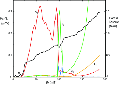
Figure 4: The torque increase and variance of induced field coefficients as the applied field is varied. We characterize the saturated state by the mode with the largest variance. These measurements were taken for a fixed rotation rate of $30$ Hz ($R_{m}=16$). The field data reflect fluctuations in the coefficients from their means, except the E0 state which shows significant mean amplitude (squared average shown in green, variance of fluctuations in blue), and does so at the same applied field values where it shows ample fluctuations. At zero field, the base state torque (including confounding errors due to seals) here is $1.14$ N-m, the black curve shows the increase in torque above this base value.

Also shown in Fig. 5 are predicted magnetorotational stability boundaries, as obtained from an inviscid dispersion relation ji ; goodman adapted to the present configuration. The two curves represent the stability boundaries of modes with $kb=1$ (red) and $kb=2$ (blue) for wavenumber $k$, i.e. wavelengths of one or one-half a circumference. We take the peak rotation rate $\Omega_{p}$ in the dispersion relation to be an estimated fluid rotation just outside the inner boundary layer $\Omega_{p}=\Omega_{o}/3$. The correlation between the predicted stability boundaries and the experimental observation of the magnetic field oscillations with progressively more spatial structure is strong evidence that we have observed the magnetorotational instability in our experiment.

These measurements, beyond being the first direct observation of the magnetorotational instability in a physical system, have important implications for our understanding of magnetohydrodynamic instabilities. They establish that the magnetorotational instability, and a significant increase in angular momentum transport, occur in the presence of pre-existing hydrodynamic turbulence. We quantify the nonlinear saturated amplitude of the angular momentum transport and the patterns and saturated values of magnetic field over a range of parameter values not computationally accessible. Finally, this geometry may well be capable, at high $R_{m}$, of showing a dynamo instability. While the dynamo instability is distinct from the magnetorotational instability, it would be important to examine a system capable of showing both.

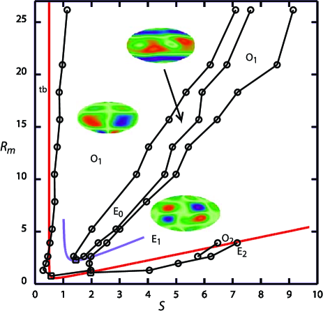
Figure 5: Phase diagram of saturated states. Regions are defined by the mode with the largest variance of fluctuations (see Fig. 4). Some secondary instabilities show hysteresis; these data are for increasing $S$, for fixed $R_{m}$. The states have regions associated with background turbulence (tb), mode O1 dominated, E0 dominated, followed by O1, E1, O2, and E2 modes. The lowest $R_{m}$ and $S$ numbers for these states ($\square$) are obtained by extrapolating the maximum saturated state amplitude versus $R_{m}$ (a linear trend) to zero amplitude. Also shown are theoretical stability boundaries for the longest wavelength (red) and second longest wavelength (blue) instabilities, calculated from the magnetorotational dispersion relation.

- (1)
- (2) S.A. Balbus and J.F. Hawley, Astrophys. J. 376, 214 (1991).
- (3) S.A. Balbus and J.F. Hawley, Rev. Mod. Phys. 70, 1 (1998).
- (4) S.A. Balbus, Annu. Rev. Astron. Astrophys. 41, 555 (2003).
- (5) E.P. Velikhov, Sov. Phys. JETP 36, 1398 (1959).
- (6) S. Chandrasekhar, Proc. Natl. Acad. Sci. USA 46, 253 (1960).
- (7) S. Chandrasekhar, Hyrodynamic and Hydromagnetic Stability, (Dover, New York, 1961).
- (8) J.E. Pringle, Ann. Rev. of Astro. and Astrophys. 19, 137 (1981).
- (9) D.S. Krasnov, E. Zienicke, O. Zikanov, T. Boeck, and A. Thess, J. Fluid Mech. 504, 183 (2004).
- (10) P. Moresco and T. Alboussiere, J. Fluid Mech. 504, 167 (2004).
- (11) Y. Ponty, H. Politano, and J.-F. Pinton Phys. Rev. Lett. 92, 144503 (2004).
- (12) S.A. Balbus and J.F. Hawley, Mon. Not. R. Astron. Soc. 266, 769 (1994).
- (13) L.L. Kitchatinov and G. Rüdiger, Mon. Not. R. Astron. Soc. 286, 757 (1997).
- (14) M.C. Begelman, Science 300, 1898 (2003).
- (15) J.F. Hawley, S.A. Balbus and J.M. Stone, Astrophys. J. 554, L49 (2001).
- (16) R.J. Donnelly and M. Ozima, Phys. Rev. Lett. 4, 497 (1960).
- (17) The experiments were carried out in liquid sodium temperature controlled to C.
- (18) N.L. Peffley, A.B. Cawthorne and D.P. Lathrop, Phys. Rev. E 61, 5287 (2000).
- (19) The induced field data from the 30 probe array were projected onto the poloidal vector spherical harmonics of orders one through four using least squares, giving 24 Gauss coefficients: one per axisymmetric mode, two per nonzero m mode. Typical experiments consisted of increasing the applied field from ambient to the maximum external field (typically 0.20 T) in 2.2 mT increments for a fixed rotation rate.
- (20) Y. Takeda, Nuc. Eng. and Design 126, 277 (1991).
- (21) The velocity measurements were obtained using pulsed ultrasound Doppler velocimetry at 4 MHz. Oxide particles that occur inevitably in our sodium scatter sound and track the flow takeda . We constructed an ultrasound transducer with a PTFE surface coated by a thin film of silicon rubber in order to ensure good wetting with the sodium. The chord of velocity measurements was 0.063 m below the equatorial plane and off axis by 0.043 m at the nearest point.
- (22) P.A. Davidson, An Introduction to Magnetohydrodynamics, (Cambridge Univ. Press, Cambridge, 2001), pp. 417.
- (23) D.R. Sisan, W.L. Shew and D.P. Lathrop, Phys. Earth and Planet. Int. 135, 137 (2003).
- (24) H. Ji, J. Goodman and A. Kageyama, Mon. Not. R. Astron. Soc. 325, L1 (2001).
- (25) J. Goodman and H. Ji, J. Fluid Mech. 462, 365 (2002).
- (26) E. Bullard and H. Gellman, Proc. Roy. Sec. A 247, 213 (1954).
- (27) W.T. Kim and E.C. Ostriker, Astrophys. J. 540, 372 (2000).
- (28) K. Noguchi, V.I. Pariev, S.A. Colgate, H.F. Beckley and J. Nordhaus, Astrophys. J. 575, 1151 (2002).
- (29) E. Knobloch, Phys. Fluids 8, 1446 (1996).
- (30) R. Hollerbach and S. Skinner, Proc. Roy. Soc. Lon. A 257, 785 (2001).