Dynamic Models and Nonlinear Filtering
of Wave Propagation in Random Fields

Abstract

In this paper, a general model of wireless channels is established based on the physics of wave propagation. Then the problems of inverse scattering and channel prediction are formulated as nonlinear filtering problems. The solutions to the nonlinear filtering problems are given in the form of dynamic evolution equations of the estimated quantities. Finally, examples are provided to illustrate the practical applications of the proposed theory.

Keywords: channel estimation and prediction, nonlinear filtering, fast fading, random field.

1 Introduction

In modern engineering, the problem of modeling wave propagation in a random field of scattering objects and of the associated signal processing, has become more and more important, with wide applications ranging from wireless communications, to radar or sonar object detection, to medical imaging using microwave or infrared light. In all of the applications, the first thing is obviously to understand and model the wave propagation in random fields. In the object detection and imaging applications, the signal processing is usually an inverse scattering problem, that is to find out the configuration and dynamics of the scattering objects in the random field, based on the data of received signals and the known transmitted signal. When applied to the field of wireless communications, for instance, channel estimation and prediction for dynamic power control or adaptive modulation, the problem goes one step deeper and becomes filtering and predicting the dynamics of the channel response, given some observed data of the past channel response. A powerful model of wave propagation will be established based upon the physics of wave scattering, by which the channel response may be computed explicitly as a functional of the random field of scattering objects. Then, it becomes natural to approach the problem of estimating and predicting the channel response in two steps: solving the inverse scattering problem first, then calculating the channel response using the solved dynamics of the scattering objects.

Such a natural two-step approach seems to have been overlooked in the existing literature of communications. In fact, the traditional approaches try to avoid the inverse scattering problem. They often start directly from some presumed stochastic models of the channel response, without looking into the actual random field of scattering objects at all. In the Rayleigh fading model that has been widely used since the early days of wireless communications [1], the physical scattering environment is absent from the consideration, while the received signal is assumed to be a sum of many differently delayed and weighted versions of the transmitted signal, where the weighting coefficients are complex Gaussian and independent, the delay times modulo $1/f_{c}$ are also independent and uniformly distributed in $[0,1/f_{c})$, with $f_{c}$ being the center frequency of the carrier [2]. When there is one strong, dominating component, e.g. from line-of-sight propagation, the Rayleigh model is slightly modified into the Ricean fading model. Both models are based on the assumption of a large number of scattering objects, which may not always be the case. In case an adaptive mechanism is employed to control the transmitter power or vary the transmission bit rate, the channel estimation and prediction circuit has to be very fast to follow the dynamics of the channel response [3]. The previous channel models have become inadequate in millimeter wave mobile communications, where the channel is fast-fading, namely, the bit duration is short comparing to the dynamics of channel response [4]. In fact, the inadequacy of the old models may be held responsible for a general opinion among many wireless engineers that in many fast-fading systems, it might be impossible to estimate the channel state information (CSI) so to adapt the system accordingly [5]. Such a pessimistic view has even inspired a lot of work concerning the capacity and coding schemes of future high speed and fast-fading wireless channels [5, 6]. A generally used estimation of the fading speed is based upon the assumption that the signal fading experienced by two receivers become uncorrelated when the separation between the receivers is significantly larger than the carrier wavelength [7]. However, in the Rayleigh or Ricean model, the signal fading is governed by a Gaussian law of distribution, which implies the equivalence between uncorrelation and independence. So even in principle, the signal fading seen in one region does not contain any information for the signal fading in another region just a few wavelengths away. This imposes a serious limitation upon the estimation of CSI. For instance, consider a wireless link with the carrier frequency around 1.9 GHz, so the wavelength is about 0.158 meter. It takes merely 8 milliseconds for a mobile with speed 20 m/s to travel through one wavelength. It seems, according to the Rayleigh and Ricean models, that an estimator for the CSI has to accomplish its task well within a millisecond, and the obtained CSI can be regarded as reliable for no longer than 8 milliseconds.

We think that the above limit on the CSI estimation of a fast-fading channel is over pessimistic. Our point of view is that for any wireless link in a given physical environment, the channel response is the result of the superposition of waves propagating via multiple paths, where each signal path is a geometric route that starts from the transmitter, possibly hits one or more scattering objects, and finally reaches the transmitter. The physical environment that contains the scattering objects is called a scattering environment. The response of a wireless channel is actually deterministic, conditioned upon the scattering environment and the locations of the transmitter and receiver inside the scattering environment. The randomness of wireless channels arises only from the variety of scattering environments. In a wireless channel model based on the physics of wave propagation in a scattering environment, a natural choice for the “channel state” would be the state of the scattering environment, namely the positions and velocities of the scattering objects as well as their physical effects on the wave. So the estimation of CSI boils down to estimating the positions, velocities, and attenuation coefficients of the scattering objects. Such channel state should remain largely time-invariant over a much longer time period. As an example, consider a scattering environment in which the distance among the scattering objects, the transmitter, and the receiver is at least several tens of meters, so that the mobile receiver or transmitter experiences the same scattering environment even after it travels over 10 meters. With the 20 m/s mobile speed, it takes 0.5 second to cover that distance, which is more than 60 wavelengths for a carrier frequency around 1.9 GHz.

There have been previous works adopting a deterministic model of signal fading [8, 9, 10], but in most of them the effect of the scattering environment is represented by a superposition of plane waves in proximity to the receiver, whose interference pattern is sampled by the receiver. This representation only works for a frequency-nonselective channel [2], where the frequency bandwidth of the signal is too narrow to resolve the delay times of different paths. When the signal bandwidth is sufficiently large to resolve the path delays, the plane wave representation breaks down, a more advanced model that captures both the direction of arrivals and the path delays is necessary. Moreover, the previous works [8, 9, 10] estimate the CSI using various spectral estimation techniques, which do not guarantee the optimality of the solutions. In this paper, we shall first establish a complete model of wireless channels based on the physics of wave propagation. Then the problems of inverse scattering and channel prediction are formulated as nonlinear filtering problems. The solution to the nonlinear filtering problem will be given in the form of a dynamic evolution equation (the filtering equation) for the estimated quantities, just like the Kalman filtering equation for the linear filtering problem [11]. In most practical applications, the filter equation may be implemented, or at least be approximated, by a state-possessing machine driven by an innovation input. In our particular applications, it happens that both the state of the scattering environment and the observation process are governed by linear differential equations. Note that even though the system equations are linear, the Kalman filter may still be sub-optimal, unless the initial probability law of the system state is Gaussian. It is proven mathematically that the nonlinear filter produces the optimal estimation for the interested quantity. Even the nonlinear filter may not be easily implemented in practice, its solution provides a benchmark for evaluating the performance of other sub-optimal estimators. The theory of nonlinear filtering has been well established, many textbooks exist, covering its fundamental principles and applications, especially to the field of control engineering [12, 13, 14], however it has not made much appearance in the field of communication engineering. Apart from an attempt to solve the channel prediction problem for fast-fading wireless channels, the present paper is intended to introduce the nonlinear filtering theory as a powerful tool for signal processing and system optimization in the field of communication engineering.

2 Random Scattering Fields and Wave Propagation Therein

Throughout the present paper, a sufficiently large probability space $(\Omega,{\cal F},P)$ is assumed in which all random variables under consideration are defined. In the wave-involved applications mentioned in the beginning of the introduction, there is often a random scattering field (RSF) consisting of scattering objects, due to which the signal wave from a transmitter to a receiver undergoes multiple scattering and propagates along various geometric paths associated with different power losses, different time delays and direction of arrivals, as pictured in Fig.1. The spatial domain ${\cal E}\subseteq{\rm I\kern-1.79993ptR}^{q}$ accommodating the scattering objects together with the signal transmitter and the receiver is called the scattering environment, where $q\in{\rm I\kern-1.79993ptN}$ is the dimension of the space under consideration, usually $q=2$ or $3$. In general, an RSF, denoted by $S(t;{\bf r},{\bf v})$, may contain spatially extensive scattering objects, which could be continuously distributed in the real space and the velocity space, namely the configuration space. Fig.1 only shows a special RSF with discrete scattering objects, which may be the most adopted model [15, 16]. A discrete RSF is often modeled by a compound point process [17, 18] in the configuration space ${\cal E}\times{\rm I\kern-1.79993ptR}^{q}$,

$$S(t;{\bf r},{\bf v})=\sum_{k=3}^{N(t)}S_{k}\delta({\bf r}-{\bf r}_{k})\delta({\bf v}-{\bf v}_{k}),$$ (1)

where ${\bf r}=(r_{1},\cdots,r_{q})^{\prime}\in{\cal E}$ and ${\bf v}=(v_{1},\cdots,v_{q})^{\prime}\in{\rm I\kern-1.79993ptR}^{q}$ denote the position and the velocity respectively, and hence $\{({\bf r}_{k},{\bf v}_{k})\}_{k=3}^{N(t)}$ are configuration coordinates for the scattering objects, which are the realization points of a space-time point process in $[0,\infty)\times{\cal E}\times{\rm I\kern-1.79993ptR}^{q}$. Here $N(t)$ is the total number of points occurred up to time $t$ anywhere in ${\cal E}\times{\rm I\kern-1.79993ptR}^{q}$. The scattering objects are indexed by the integers $k\geq 3$, the indices $k=1,2$ are reserved for the transmitter and the receiver respectively. For each $k\geq 3$, $S_{k}$ is a complex-valued random variable associated with the $k$th realization point, which represents the scattering response of the corresponding scattering object to the signal. Although the discrete RSF model is chosen here to simplify the discussion, it should be pointed out that, a more general RSF model might, and should be used when necessary, for example, when describing a scattering environment with continuously distributed scattering objects. In fact, all mathematical formulae with $S(t;{\bf r},{\bf v})$ involved in the present paper are formulated in such general forms that they hold for any ${\cal D}^{\prime}({\cal E}\times{\rm I\kern-1.79993ptR}^{q})$-valued process $S(t;{\bf r},{\bf v})$, where ${\cal D}^{\prime}({\cal E}\times{\rm I\kern-1.79993ptR}^{q})$ denotes the Hilbert space of the complex-valued, linear functionals of functions in ${\cal E}\times{\rm I\kern-1.79993ptR}^{q}$, which are usually called distributions or generalized functions [19, 20].

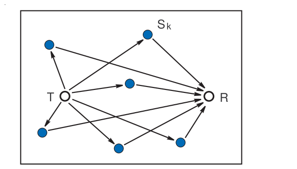
Figure 1: A typical random scattering field, in which the signal wave propagates from a transmitter to a receiver along various geometric paths as a result of the interaction with the scattering objects.

The RSF imprints itself on the channel response between a wave transmitter and a signal receiver, all of which lie in the scattering environment ${\cal E}$. In general, both the transmitter and the receiver could be extensive in space, as being the case when antenna arrays are employed. Therefore we use $x(t;{\bf r}_{1},{\bf v}_{1})$ and $y(t;{\bf r}_{2},{\bf v}_{2})$ to denote the spatially extensive signal amplitudes of the transmitter and the receiver respectively, both of which are complex-valued and square integrable in the Lebesgue sense, namely, $x,y\in L^{2}([0,\infty)\times{\cal E}\times{\rm I\kern-1.79993ptR}^{q},{\cal C})$, where ${\cal C}$ is the set of complex numbers. Recalling the theory of wave scattering which says that the otherwise freely propagating signal wave from a source is perturbed by the scattering objects, and the actual wave in space is the superposition of the free-running wave and all of the scattered waves. The Huygens-Fresnel principle [21, 22] further states that the scattered wave from each scattering object, often called the second wave, is again a free-running wave coming out of the object, with an amplitude proportional to that of the incident wave, and the proportional coefficient is called the scattering response of the object. In general, it is rather complicated to calculate the actual wave in an exact manner, which involves the solution of an integral equation or a series expansion using the Feynman diagram [23, 24]. The complication has to do with the multiple scattering effects. However, when the scattering objects are sparsely distributed in space, their effect on the signal wave may be easily calculated using the perturbation theory. In particular, the first-order perturbation theory approximates the actual wave by superposing the free-running wave and the second waves excited by it at the scattering objects. For an obvious reason, the first-order perturbation is also called the single-bounce approximation. When considering only the contribution of the second waves, the single-bounce approximation results in an input-output relation of the spatially extensive signals $x(t;{\bf r}_{1},{\bf v}_{1})$ and $y(t;{\bf r}_{2},{\bf v}_{2})$ in their low-pass equivalent form [2],

$$y(t;{\bf r}_{2},{\bf v}_{2})=\sum_{k=3}^{N(t)}\int_{{\cal E}\times{\rm I\kern-1.25995ptR}^{q}}x(t-\tau_{1k}-\tau_{k2};{\bf r}_{1},{\bf v}_{1})l(c\tau_{1k})S_{k}l(c\tau_{k2})\exp(i2\pi\gamma_{1k2}t)d{\bf r}_{1}d{\bf v}_{1},$$ (2)

where $\tau_{1k}$ and $\tau_{k2}$ are the time delays associated with the signal propagation from the transmitter to the $k$th object and from the $k$th object to the receiver respectively, which satisfy the following equations,

$$\tau_{1k}=\frac{|{\bf r}_{1}-{\bf r}_{k}(t-\tau_{k2})|}{c},~{}\tau_{k2}=\frac{|{\bf r}_{k}(t-\tau_{k2})-{\bf r}_{2}|}{c},~{}\forall~{}k\geq 3.$$ (3)

Also in the above equations, $c$ is the speed of the wave, $l(c\tau)$ is the propagation loss that depends only on the propagation distance $c\tau$, and

$$\gamma_{1k2}\stackrel{{\scriptstyle\mathrm{d}ef}}{{=}}\frac{f_{0}[{\bf v}_{1}-{\bf v}_{k}(t-\tau_{k2})]\cdot[{\bf r}_{1}-{\bf r}_{k}(t-\tau_{k2})]}{c|{\bf r}_{1}-{\bf r}_{k}(t-\tau_{k2})|}+\frac{f_{0}[{\bf v}_{k}(t-\tau_{k2})-{\bf v}_{2}]\cdot[{\bf r}_{k}(t-\tau_{k2})-{\bf r}_{2}]}{c|{\bf r}_{k}(t-\tau_{k2})-{\bf r}_{2}|},$$ (4)

is the Doppler frequency shift experienced by the signal with the central carrier frequency $f_{0}$. Note that the time delays $\{\tau_{k2}\}_{k\geq 3}$ are implicitly defined in equation (3), although an explicit formula may be derived when the kinetic motions of the scattering objects are given explicitly. For example, if the velocity difference ${\bf v}_{k}(t)-{\bf v}_{k}(t-\tau_{k2})$ is neglected for all $k\geq 3$, that is to ignore the velocity variation during the time of the wave propagating from the scattering object to the receiver, then the following equation holds,

$$c\tau_{k2}=|{\bf r}_{k}(t)-{\bf v}_{k}(t)\tau_{k2}-{\bf r}_{2}|,~{}\forall~{}k\geq 3,$$ (5)

which is easily solved to give an explicit formula,

$$\tau_{k2}=\frac{\sqrt{[c^{2}-|{\bf v}_{k}(t)|^{2}]|{\bf r}_{k}(t)-{\bf r}_{2}|^{2}+\{[{\bf r}_{k}(t)-{\bf r}_{2}]\cdot{\bf v}_{k}(t)\}^{2}}-[{\bf r}_{k}(t)-{\bf r}_{2}]\cdot{\bf v}_{k}(t)}{c^{2}-|{\bf v}_{k}(t)|^{2}},~{}\forall~{}k\geq 3.$$ (6)

Then the time delays $\{\tau_{1k}\}_{k\geq 3}$ are explicitly computed using equations (3) and (6). Similarly, equation (4) could be simplified if all $\{{\bf v}_{k}\}_{k\geq 3}$ are treated as constants during the interval $[t-\tau_{k2},t]$,

$$\gamma_{1k2}\stackrel{{\scriptstyle\mathrm{d}ef}}{{=}}\frac{f_{0}[{\bf v}_{1}-{\bf v}_{k}(t)]\cdot[{\bf r}_{1}-{\bf r}_{k}(t)+{\bf v}_{k}(t)\tau_{k2}]}{c|{\bf r}_{1}-{\bf r}_{k}(t)+{\bf v}_{k}(t)\tau_{k2}|}+\frac{f_{0}[{\bf v}_{k}(t)-{\bf v}_{2}]\cdot[{\bf r}_{k}(t)-{\bf v}_{k}(t)\tau_{k2}-{\bf r}_{2}]}{c|{\bf r}_{k}(t)-{\bf v}_{k}(t)\tau_{k2}-{\bf r}_{2}|},~{}\forall~{}k\geq 3.$$ (7)

Neglecting the object velocity variation during the time of wave propagation is often an excellent approximation to make, especially when dealing with electromagnetic waves, which travel at the ultimate speed in nature, $c=3.0\times 10^{8}$ m/s. Even for ten kilometers of propagation distance, the time delay is merely $1/30$ millisecond, during which no macroscopic scattering object can change its speed for much. Furthermore, the highest speed of most macroscopic objects is no more than a millionth of the light speed. Consequently, equation (6) may be simplified,

$$\tau_{k2}=\frac{|{\bf r}_{k}(t)-{\bf r}_{2}|}{c}-\frac{[{\bf r}_{k}(t)-{\bf r}_{2}]\cdot{\bf v}_{k}(t)}{c^{2}},~{}\forall~{}k\geq 3,$$ (8)

by neglecting terms of the second or higher powers of ${\bf v}_{k}(t)/c$, $\forall~{}k\geq 3$. Or even simpler, while still an extremely good approximation for the propagation of electromagnetic wave, the time delays may be calculated as,

$$\tau_{1k}=\frac{|{\bf r}_{1}-{\bf r}_{k}(t)|}{c},~{}\tau_{k2}=\frac{|{\bf r}_{k}(t)-{\bf r}_{2}|}{c},~{}\forall~{}k\geq 3.$$ (9)

To write the input-output relation in a more compact form, we define

$$\tau_{2}({\bf r},{\bf v};{\bf r}_{2})\stackrel{{\scriptstyle\mathrm{d}ef}}{{=}}\frac{\sqrt{(c^{2}-|{\bf v}|^{2})|{\bf r}-{\bf r}_{2}|^{2}+[({\bf r}-{\bf r}_{2})\cdot{\bf v}]^{2}}-({\bf r}-{\bf r}_{2})\cdot{\bf v}}{c^{2}-|{\bf v}|^{2}},~{}\forall~{}k\geq 3,$$ (10)

$$\tau_{1}({\bf r}_{1};{\bf r},{\bf v};{\bf r}_{2})\stackrel{{\scriptstyle\mathrm{d}ef}}{{=}}\frac{|{\bf r}_{1}-{\bf r}+{\bf v}\tau_{2}({\bf r},{\bf v};{\bf r}_{2})|}{c},~{}\forall~{}k\geq 3,$$ (11)

$$\gamma({\bf r}_{1},{\bf v}_{1};{\bf r},{\bf v};{\bf r}_{2},{\bf v}_{2})\stackrel{{\scriptstyle\mathrm{d}ef}}{{=}}\frac{f_{0}({\bf v}_{1}-{\bf v})\cdot[{\bf r}_{1}-{\bf r}+{\bf v}\tau_{2}({\bf r},{\bf v};{\bf r}_{2})]}{c|{\bf r}_{1}-{\bf r}+{\bf v}\tau_{2}({\bf r},{\bf v};{\bf r}_{2})|}+\frac{f_{0}({\bf v}-{\bf v}_{2})\cdot[{\bf r}-{\bf v}\tau_{2}({\bf r},{\bf v};{\bf r}_{2})-{\bf r}_{2}]}{c|{\bf r}-{\bf v}\tau_{2}({\bf r},{\bf v};{\bf r}_{2})-{\bf r}_{2}|},$$ (12)

$$L({\bf r}_{1},{\bf v}_{1};{\bf r},{\bf v};{\bf r}_{2},{\bf v}_{2})\stackrel{{\scriptstyle\mathrm{d}ef}}{{=}}l[c\tau_{1}({\bf r}_{1};{\bf r},{\bf v};{\bf r}_{2})]l[c\tau_{2}({\bf r},{\bf v};{\bf r}_{2})]\exp[i2\pi\gamma({\bf r}_{1},{\bf v}_{1};{\bf r},{\bf v};{\bf r}_{2},{\bf v}_{2})],$$ (13)

then we use equation (1), together with equations (6), and (7) to rewrite equation (2) as,

$$y(t;{\bf r}_{2},{\bf v}_{2}) = \int_{({\cal E}\times{\rm I\kern-1.25995ptR}^{q})^{2}}x[t-\tau_{1}({\bf r}_{1};{\bf r},{\bf v};{\bf r}_{2})-\tau_{2}({\bf r},{\bf v};{\bf r}_{2});{\bf r}_{1},{\bf v}_{1}]$$ (14)

$$\times L({\bf r}_{1},{\bf v}_{1};{\bf r},{\bf v};{\bf r}_{2},{\bf v}_{2})S[t-\tau_{2}({\bf r},{\bf v};{\bf r}_{2});{\bf r},{\bf v}]d{\bf r}_{1}d{\bf v}_{1}d{\bf r}d{\bf v}.$$

This equation shall serve as the fundamental input-output relation describing the propagation of spatially extensive signals in an RSF, up to the single-bounce approximation. It is evident that the received signal $y(t;{\bf r}_{2},{\bf v}_{2})$ is a bilinear functional of $x(t;{\bf r}_{1},{\bf v}_{1})$ and $S(t;{\bf r},{\bf v})$, for any fixed $(t;{\bf r}_{2},{\bf v}_{2})$. More specifically, $y(t;{\bf r}_{2},{\bf v}_{2})$ is a linear functional of $x(t;{\bf r}_{1},{\bf v}_{1})$, if $L({\bf r}_{1},{\bf v}_{1};{\bf r},{\bf v};{\bf r}_{2},{\bf v}_{2})S(t;{\bf r},{\bf v})$ is regarded as an integration kernel; or $y(t;{\bf r}_{2},{\bf v}_{2})$ could be viewed as a linear functional of $S(t;{\bf r},{\bf v})$, with $x(t;{\bf r}_{1},{\bf v}_{1})L({\bf r}_{1},{\bf v}_{1};{\bf r},{\bf v};{\bf r}_{2},{\bf v}_{2})$ serving as an integration kernel.

3 The Dynamics of RSF

Let us consider the case in which the set of scattering objects is fixed in time and the scattering response of each object is time-independent. Nevertheless, the RSF is still time-varying when the objects are subject to kinetic motion. We shall employ an RSF model so general that the scattering objects are subject to accelerations that depend upon the position. Specifically, the motion of the $k$th scattering object, $k\geq 3$, is described by a differential equation,

$$d{\bf r}_{k} = {\bf v}_{k}dt,$$ (15)

$$d{\bf v}_{k} = f({\bf r}_{k})dt,$$ (16)

where $f({\bf r})$ is an ${\rm I\kern-1.79993ptR}^{q}$-valued function representing the deterministic acceleration exerted upon the scattering objects. Since the total number of scattering objects within the environment ${\cal E}$ is assumed to be fixed in time, it is a random variable $N=N(\omega)$. As mentioned before, all random variables and processes are defined on the “grand” probability space $(\Omega,{\cal F},P)$. Let

$$S(t;{\bf r},{\bf v})\stackrel{{\scriptstyle\mathrm{d}ef}}{{=}}\sum_{k=3}^{N}S_{k}\delta({\bf r}-{\bf r}_{k})\delta({\bf v}-{\bf v}_{k}),$$ (17)

then $S(t;{\bf r},{\bf v})$ is a space-time compound point process [17, 18] in the space $[0,\infty)\times{\cal E}\times{\rm I\kern-1.79993ptR}^{q}$. Let $U$ denotes the Hilbert space of all generalized functions in ${\cal E}\times{\rm I\kern-1.79993ptR}^{q}$, namely $U\stackrel{{\scriptstyle\mathrm{d}ef}}{{=}}{\cal D}^{\prime}({\cal E}\times{\rm I\kern-1.79993ptR}^{q})$, then $S(t;{\bf r},{\bf v})$ may also be viewed as a $U$-valued random process indexed by $t\in[0,\infty)$. Next we attempt to derive a partial differential equation for $S(t;{\bf r},{\bf v})$ using equations (15), (16) and (17).

While explicitly parameterized by ${\bf r}$ and ${\bf v}$, the RSF $S(t;{\bf r},{\bf v})$ of equation (17) is implicitly a function of the processes $\{({\bf r}_{k},{\bf v}_{k})\}_{k=3}^{N}$, described by the differential equations (15) and (16). By differentiating equation (17), it is obtained that,

$$dS(t;{\bf r},{\bf v}) = \sum_{k}S_{k}\delta({\bf v}-{\bf v}_{k})d\delta({\bf r}-{\bf r}_{k})+\sum_{k}S_{k}\delta({\bf r}-{\bf r}_{k})d\delta({\bf v}-{\bf v}_{k})$$ (18)

$$= \sum_{k}S_{k}\delta({\bf v}-{\bf v}_{k})\frac{\partial\delta({\bf r}-{\bf r}_{k})}{\partial{\bf r}_{k}}{\bf v}_{k}dt+\sum_{k}S_{k}\delta({\bf r}-{\bf r}_{k})\frac{\partial\delta({\bf v}-{\bf v}_{k})}{\partial{\bf v}_{k}}f({\bf r}_{k})dt$$

$$= -\sum_{k}S_{k}\delta({\bf v}-{\bf v}_{k})\frac{\partial\delta({\bf r}-{\bf r}_{k})}{\partial{\bf r}}{\bf v}_{k}dt-\sum_{k}S_{k}\delta({\bf r}-{\bf r}_{k})\frac{\partial\delta({\bf v}-{\bf v}_{k})}{\partial{\bf v}}f({\bf r}_{k})dt$$

$$= -\sum_{k}S_{k}\delta({\bf v}-{\bf v}_{k})\frac{\partial\delta({\bf r}-{\bf r}_{k})}{\partial{\bf r}}{\bf v}dt-\sum_{k}S_{k}\delta({\bf r}-{\bf r}_{k})\frac{\partial\delta({\bf v}-{\bf v}_{k})}{\partial{\bf v}}f({\bf r})dt,$$

for all $k\geq 3$, where in the last step, two identities have been used,

$$\delta({\bf v}-{\bf v}_{k}){\bf v}_{k} \equiv \delta({\bf v}-{\bf v}_{k}){\bf v},~{}\forall~{}k\geq 3,$$ (19)

$$\delta({\bf r}-{\bf r}_{k})f({\bf r}_{k}) \equiv \delta({\bf r}-{\bf r}_{k})f({\bf r}),~{}\forall~{}k\geq 3.$$ (20)

The partial differential operator $\partial/\partial{\bf r}$ is defined as a row vector,

$$\frac{\partial}{\partial{\bf r}}\stackrel{{\scriptstyle\mathrm{d}ef}}{{=}}\left[\frac{\partial}{\partial r_{1}},\cdots,\frac{\partial}{\partial r_{q}}\right],$$ (21)

and the operator $\partial/\partial{\bf v}$ is similarly defined. Note that $f({\bf r})$ is valued as a $q$-dimensional column vector. When a row vector is followed by a column vector, it is understood that the scalar product in the space ${\rm I\kern-1.79993ptR}^{q}$ takes place. Noticing two more identities,

$$\frac{\partial S(t;{\bf r},{\bf v})}{\partial{\bf r}} = \sum_{k}S_{k}\delta({\bf v}-{\bf v}_{k})\frac{\partial\delta({\bf r}-{\bf r}_{k})}{\partial{\bf r}},$$ (22)

$$\frac{\partial S(t;{\bf r},{\bf v})}{\partial{\bf v}} = \sum_{k}S_{k}\delta({\bf r}-{\bf r}_{k})\frac{\partial\delta({\bf v}-{\bf v}_{k})}{\partial{\bf v}},$$ (23)

one may easily simplify equation (18) into a partial differential equation governing the RSF,

$$dS(t;{\bf r},{\bf v})=-\frac{\partial S(t;{\bf r},{\bf v})}{\partial{\bf r}}{\bf v}dt-\frac{\partial S(t;{\bf r},{\bf v})}{\partial{\bf v}}f({\bf r})dt.$$ (24)

Define a linear operator $A:U\rightarrow U$, such that for any $\xi\in U$,

$$A\xi({\bf r},{\bf v})\stackrel{{\scriptstyle\mathrm{d}ef}}{{=}}-\frac{\partial\xi}{\partial{\bf r}}{\bf v}-\frac{\partial\xi}{\partial{\bf v}}f({\bf r}),$$ (25)

then equation (24), together with a proper initial condition, is immediately recognized as an infinite dimensional linear system [25, 26] in the Hilbert space $U$,

$$dS(t) = AS(t)dt,$$ (26)

$$S(0) = S_{0},$$ (27)

where $S_{0}$ is an $({\cal F},{\cal B}(U))$-measurable random variable, ${\cal B}(U)$ is a Borel $\sigma$-algebra of subsets of $U$. It is to be stressed again that the dynamic equations (26) and (27) are applicable to any RSF $S(t)\in U={\cal D}^{\prime}({\cal E}\times{\rm I\kern-1.79993ptR}^{q})$, although the derivation of the equations is exemplified by the special case of discrete RSF for simplicity.

4 Signal Detection

As discussed in section 2, when a spatially extensive signal $x(t;{\bf r}_{1},{\bf v}_{1})$ is transmitted, a spatially extensive receiver will catch a signal $y(t;{\bf r}_{2},{\bf v}_{2})$, which may be degraded by a white Gaussian noise. Let

$$Y(t;{\bf r}_{2},{\bf v}_{2})\stackrel{{\scriptstyle\mathrm{d}ef}}{{=}}\int_{0}^{t}y(s;{\bf r}_{2},{\bf v}_{2})ds+Z(t;{\bf r}_{2},{\bf v}_{2}),$$ (28)

where $Z(t;{\bf r}_{2},{\bf v}_{2})$ is an $H$-valued Wiener process representing the observation noise, with $H\stackrel{{\scriptstyle\mathrm{d}ef}}{{=}}L^{2}({\cal E}\times{\rm I\kern-1.79993ptR}^{q})$, that is, the space of square Lebesgue integrable functions in ${\cal E}\times{\rm I\kern-1.79993ptR}^{q}$. It is also assumed that the covariance operator of $Z(t)$, denoted by $R$, is uniformly positive definite. Using equation (14), with the simplified calculation of delay times in (9), we can write,

$$dY(t;{\bf r}_{2},{\bf v}_{2}) = \left[\int_{({\cal E}\times{\rm I\kern-1.25995ptR}^{q})^{2}}x\left(t-\frac{|{\bf r}_{1}-{\bf r}|+|{\bf r}-{\bf r}_{2}|}{c};{\bf r}_{1},{\bf v}_{1}\right)L({\bf r}_{1},{\bf v}_{1};{\bf r},{\bf v};{\bf r}_{2},{\bf v}_{2})\right.$$ (29)

$$\times \left.S\left(t-\frac{|{\bf r}-{\bf r}_{2}|}{c};{\bf r},{\bf v}\right)d{\bf r}_{1}d{\bf v}_{1}d{\bf r}d{\bf v}\right]dt+dZ(t;{\bf r}_{2},{\bf v}_{2}),$$

$$Y(0) = 0,$$ (30)

which is the signal detection equation, or called the observation equation. With the observation data $\{Y(s)\}_{0\leq s<t}$, two estimation problems emerge, depending upon the actual application goal:

1)

estimating and predicting $S(t)$, when $\{x(s)\}_{0\leq s\leq t}$ is known;

2)

estimating $x(t)$, when $\{S(t)\}_{0\leq s\leq t}$ is known.

The first problem is related to various applications of inverse scattering, such as radar object detection, channel estimation and prediction for wireless communications; while the second problem is specific to signal detection, especially to the optimal design of a receiver in communications. In the present paper, we are interested in the first estimation problem, in which the signal $x(t;{\bf r}_{1},{\bf v}_{1})$ is regarded as a known quantity. Define a time-dependent linear operator $G(t):U\rightarrow H$, such that for any time-varying function $\xi(t)\in U$, $\forall~{}t\geq 0$,

$$G(t)\xi(t)({\bf r}_{2},{\bf v}_{2})\stackrel{{\scriptstyle\mathrm{d}ef}}{{=}}$$

$$\int_{({\cal E}\times{\rm I\kern-1.25995ptR}^{q})^{2}}x\left(t-\frac{|{\bf r}_{1}-{\bf r}|+|{\bf r}-{\bf r}_{2}|}{c};{\bf r}_{1},{\bf v}_{1}\right)L({\bf r}_{1},{\bf v}_{1};{\bf r},{\bf v};{\bf r}_{2},{\bf v}_{2})\xi\left(t-\frac{|{\bf r}-{\bf r}_{2}|}{c};{\bf r},{\bf v}\right)d{\bf r}_{1}d{\bf v}_{1}d{\bf r}d{\bf v},$$ (31)

then the observation equations (29) and (30) are of the form,

$$dY(t) = G(t)S(t)dt+dZ(t),$$ (32)

$$Y(0) = 0,$$ (33)

where $Y(t)$ and $Z(t)$ are $H$-valued random processes, with $H=L^{2}({\cal E}\times{\rm I\kern-1.79993ptR}^{q})$, while $G(t)$ is a time-dependent linear operator in ${\cal L}_{HS}(U,H)$, with the time-dependence originated from the known and time-varying signal $x(t)$, ${\cal L}_{HS}(U,H)$ being the space of all Hilbert-Schmidt operators from $U$ to $H$.

The system equations (26), (27) and the observation equations (32), (33) constitute a nonlinear filtering problem, that is to compute the conditional probability,

$$\Pi(t)(\psi(t))\stackrel{{\scriptstyle\mathrm{d}ef}}{{=}}{\mathrm{E}}[\psi(t,S(t))|Y(s),0\leq s\leq t],$$ (34)

where $\psi(t,\xi)\in C_{b}^{1,2}([0,\infty)\times U)$ is a given test function, which is bounded and has continuous first and second order Fréchet derivatives with respect to $t$ and $\xi$ respectively. The essence of the nonlinear filtering problem is to obtain the optimal estimation of the interested quantity $\psi(t,S(t))$, based on the observation data up to time $t$, $\{Y(s)\}_{0\leq s\leq t}$. In most practical applications, it is sufficient to obtain a dynamic evolution equation for the estimated $\psi(t,S(t))$, usually in the form a differential equation driven by the observation data, which can be implemented, or simulated, by a state-possessing machine or circuit. Accordingly, a dynamic evolution equation for the estimated quantity may be regarded as a solution to the nonlinear filtering problem. Thanks to the greatly advanced theories of nonlinear filtering and of finite and infinite dimensional systems, such dynamic evolution equations have been well established as solutions to the nonlinear filtering problems.

5 Channel Estimation and Prediction

For the general theory of nonlinear filtering, the readers are referred to the excellent textbooks [12, 13, 14] and references therein, especially the original papers. Here we shall formulate the problem in a less general form, but to suit our applications better. We are interested in an inverse scattering problem, which is recast as, given,

$$dS(t)=AS(t)dt,~{}~{}~{}~{}~{}~{}~{}~{}~{}~{}~{}~{}~{}~{}~{}~{}S(0)=S_{0},$$ (35)

$$dY(t)=G(t)S(t)dt+dZ(t),~{}~{}Y(0)=0,$$ (36)

to compute,

$$\Pi(t)(\psi(t))={\mathrm{E}}[\psi(t,S(t))|Y(s),0\leq s\leq t],$$ (37)

where $Z(t)$ is an $H$-valued Wiener process, with covariance operator $R$, which is uniformly positive definite. $S_{0}$ is an $({\cal F},{\cal B}(U))$-measurable random variable with probability measure $\Pi_{0}$. $Z(t)$ and $S_{0}$ are independent. The operators $A$ and $G(t)$ are defined in (25) and (31) respectively. Although we have successfully formulated the general inverse scattering problem as a nonlinear filtering problem for an infinite dimensional linear system, we shall not present the general solution to the problem, in order to limit the scope and length of the discussion. The general solution involves much elaborate notations and concepts in functional analysis, as well as somewhat tedious arguments of convergence, which does not seem to fit the purpose of the present paper. Interested readers, however, are referred to the literature [27, 28].

What we shall focus here, is a special case of discrete RSF with the accelerations of the scattering objects being neglected, namely, all objects are moving with constant velocities. The goal of inverse scattering is to find out the initial position ${\bf r}_{k}$ and velocity ${\bf v}_{k}$, as well as the attenuation coefficient $S_{k}$ to the wave, for each scattering object $k$, $3\leq k\leq N$, based upon the received signal $\{Y(s)\}_{0\leq s\leq t}$ and the known transmitted signal $\{x(s)\}_{0\leq s\leq t}$. However, the total number of scattering objects $N$ is usually random, and to pin down the configuration coordinates $\{({\bf r}_{k},{\bf v}_{k})\}_{k=2}^{N}$ from scratch is highly difficult. A more practical approach is to discretize the initial configuration space into small regions and label each of them by an integer $n$, $1\leq n\leq M$, then to assign a complex-valued random variable ${\sf S}_{n}$ as the scattering response to the center of the $n$th region, which is coordinated by $({\sf r}_{n},{\sf v}_{n})$. The idea is, when the initial configuration space is divided into sufficiently small regions, the scattering objects within any region $n$, $1\leq n\leq M$, become non-resolvable, their scattering responses superposed together is represented by a single scattering point sitting at the center of the region with a scattering response ${\sf S}_{n}$. The result of the discretization is to remove the coordinates of the scattering objects in the initial configuration space from the set of the unknowns, but to let the complex random variables $\{{\sf S}_{n}\}_{n=1}^{M}$ bear all the information about the scattering environment. The probability law of $\{{\sf S}_{n}\}_{n=1}^{M}$ may be obtained from some experimental data, or calculated from an empirical model of the distribution of scattering objects in an actual geographical environment [15, 16]. For instance, if the distribution of objects is quite sparce in an area, then the probability of ${\sf S}_{n}=0$ is high, for any $1\leq n\leq M$. Let

$${\sf S}\stackrel{{\scriptstyle\mathrm{d}ef}}{{=}}({\sf S}_{1},{\sf S}_{2},\cdots,{\sf S}_{M})^{\prime},$$ (38)

then ${\sf S}$ is a random variable in ${\cal C}^{M}$, whose probability law is known and denoted by $\Pi_{0}$ just as before. Since the scattering response of each object is assumed time-invariant, the RSF $S(t)$, now ${\cal C}^{M}$-valued, is time-independent,

$$dS(t)=0,~{}~{}S(0)={\sf S}.$$ (39)

The transmitter and receiver are also discrete in the configuration space, which consist $I$ and $J$ antenna elements located at $\{({\sf r}_{1i},{\sf v}_{1i})\}_{i=1}^{I}$ and $\{({\sf r}_{2j},{\sf v}_{2j})\}_{j=1}^{J}$ respectively. As a consequence, the transmitted signal $x(t)$ is a ${\cal C}^{I}$-valued signal, while the Wiener noise $Z(t)$ at the receiver and the received signal $Y(t)$ are ${\cal C}^{J}$-valued random processes,

$$x(t) \stackrel{{\scriptstyle\mathrm{d}ef}}{{=}} (x_{1}(t),x_{2}(t),\cdots,x_{I}(t))^{\prime},$$ (40)

$$Y(t) \stackrel{{\scriptstyle\mathrm{d}ef}}{{=}} (Y_{1}(t),Y_{2}(t),\cdots,Y_{J}(t))^{\prime},$$ (41)

$$Z(t) \stackrel{{\scriptstyle\mathrm{d}ef}}{{=}} (Z_{1}(t),Z_{2}(t),\cdots,Z_{J}(t))^{\prime}.$$ (42)

Again let $R(t)$ denote the covariance matrix of the Wiener process $Z(t)$, which is uniformly positive definite. Define a $J\times M$ matrix ${\sf G}(t)=\{g_{jn}(t)\}_{1\leq j\leq J,1\leq n\leq M}$, such that,

$$g_{jn}(t)\stackrel{{\scriptstyle\mathrm{d}ef}}{{=}}\sum_{i=1}^{I}x\left(t-\frac{|{\sf r}_{1i}-{\sf r}_{n}|+|{\sf r}_{n}-{\sf r}_{2j}|}{c};{\sf r}_{1i},{\sf v}_{1i}\right)L({\sf r}_{1i},{\sf v}_{1i};{\sf r}_{n},{\sf v}_{n};{\sf r}_{2j},{\sf v}_{2j}),~{}\forall~{}1\leq j\leq J,~{}\forall~{}1\leq n\leq M,$$ (43)

where the function $L$ is defined in (13), then the discrete version of the observation equation (29) is formulated as,

$$dY(t)={\sf G}(t){\sf S}dt+dZ(t),~{}~{}Y(0)=0.$$ (44)

With the trivial system equation (39) and the simple observation equation (44), the inverse scattering problem is to compute,

$$\Pi(t)(\psi(t))={\mathrm{E}}[\psi(t,S(t))|Y(s),0\leq s\leq t]={\mathrm{E}}[\psi(t,{\sf S})|Y(s),0\leq s\leq t],$$ (45)

where $\psi(t,\xi)\in C_{b}^{1,2}([0,\infty)\times{\cal C}^{M},{\cal C})$ is a given test function, which is bounded and has continuous first and second order derivatives with respect to $t$ and $\xi$ respectively. For the convenience in presenting the following filtering equations, let $B:[0,\infty)\times{\cal C}^{M}\rightarrow{\cal C}^{J}$ be a function such that,

$$B(t,\xi) \stackrel{{\scriptstyle\mathrm{d}ef}}{{=}} {\sf G}(t)\xi,~{}\forall~{}t\geq 0,~{}\forall~{}\xi\in{\cal C}^{M},$$ (46)

$$B^{\prime}(t,\xi) \stackrel{{\scriptstyle\mathrm{d}ef}}{{=}} \xi^{\prime}{\sf G}^{\prime}(t),~{}\forall~{}t\geq 0,~{}\forall~{}\xi\in{\cal C}^{M}.$$ (47)

It is a trivial matter to verify the conditions in order to apply the Kushner-Stratonovitch equation [12, 13],

$$d\Pi(t)(\psi(t)) = \Pi(t)\left(\frac{\partial\psi}{\partial t}\right)dt+\left[\Pi(t)(B^{\prime}(t)\psi(t))-\Pi(t)(\psi(t))\Pi(t)(B^{\prime}(t))\right]$$ (48)

$$\times R^{-1}(t)[dY(t)-\Pi(t)(B(t))dt],~{}\mbox{\rm almost surely},~{}\forall~{}t>0,$$

$$\Pi(0)(\psi(0)) = \Pi_{0}(\psi(0))=\int_{{\cal C}^{M}}\psi(0,\xi)d\Pi_{0}(\xi).$$ (49)

Another well known solution to the nonlinear filtering problem is the Zakai equation [12, 13], which governs the so-called unnormalized conditional probability $p(t)(\psi(t))$,

$$dp(t)(\psi(t)) = p(t)\left(\frac{\partial\psi}{\partial t}\right)dt+p(t)(B^{\prime}(t)\psi(t))R^{-1}(t)dY(t),~{}\mbox{\rm almost surely},~{}\forall~{}t>0,$$ (50)

$$p(0)(\psi(0)) = \Pi_{0}(\psi(0))=\int_{{\cal C}^{M}}\psi(0,\xi)d\Pi_{0}(\xi).$$ (51)

The relation between $p(t)$ and $\Pi(t)$ is given by,

$$\Pi(t)(\psi)=\frac{p(t)(\psi)}{p(t)(1)},~{}\forall~{}\mbox{\rm test function}~{}\psi,$$ (52)

where $p(t)(1)$ satisfies,

$$dp(t)(1) = p(t)(B^{\prime}(t))R^{-1}(t)dY(t),~{}\mbox{\rm almost surely},~{}\forall~{}t>0,$$ (53)

$$p(0)(1) = 1.$$ (54)

As a simpler example, consider a flat-fading channel from a single transmitter element to a single receiver element, where the frequency bandwidth of the channel is sufficiently narrow that the time delays among the signal paths are insignificant, however, the channel response experiences a fast oscillation due to the motion of the receiver, or the transmitter, or the scattering objects. The goal is to estimate the channel state and to predict the channel response, based on the known transmitted signal and the data of received signal. This problem has been tackled before with the help of various spectral estimation techniques [8, 9, 10], which do not guarantee the optimality of the solutions. It is therefore of great interest to formulate the problem using the language of nonlinear filtering, and to see what kind of optimal solution may be obtained. The observation equation, namely, the channel input-output relation, has a very simple low-pass equivalent form [2],

$$dY(t)=x(t)h(t)dt+dZ(t),~{}~{}Y(0)=0,$$ (55)

where $x(t)$ and $Y(t)$ are the transmitted signal and the integrated version of the received signal respectively, and $h(t)$ is the time-varying channel response, all ${\cal C}$-valued, while $Z(t)$ is a ${\cal C}$-valued Wiener process with a uniformly positive definite covariance function $R(t)$. The channel response $h(t)$ is a superposition of many Doppler components,

$$h(t)=\sum_{k=1}^{K}a_{k}\exp(i2\pi f_{k}t),~{}~{}-f_{\max}\leq f_{1}<f_{2}<\cdots<f_{K}\leq f_{\max},$$ (56)

where $f_{\max}$ is the maximum Doppler frequency shift, and $\{f_{k}\}_{k=1}^{K}$ constitutes a partition of the frequency band $[-f_{\max},f_{\max}]$, and $a_{k}\in{\cal C}$ is the constant amplitude of the $k$th Doppler component, $1\leq k\leq K$. It is assumed that the partition $\{f_{k}\}_{k=1}^{K}$ is sufficiently fine to justify the discrete approximation to the Doppler shifts. Define a function $F:[0,\infty)\times{\cal C}^{K}\rightarrow{\cal C}$, such that,

$$F(t,\xi)\stackrel{{\scriptstyle\mathrm{d}ef}}{{=}}x(t)\sum_{k=1}^{K}\exp(i2\pi f_{k}t)\xi_{k},~{}\forall~{}\xi=(\xi_{1},\xi_{2},\cdots,\xi_{K})^{\prime}\in{\cal C}^{K}.$$ (57)

The nonlinear filtering problem for channel estimation and prediction is formulated as, given,

$${\sf a}\stackrel{{\scriptstyle\mathrm{d}ef}}{{=}}(a_{1},a_{2},\cdots,a_{K})^{\prime}\in{\cal C}^{K},~{}\mbox{\rm with probability law}~{}\Pi_{0},$$ (58)

$$dY(t)=F(t,{\sf a})dt+dZ(t),~{}~{}Y(0)=0,$$ (59)

to compute,

$$\Pi(t)(\psi(t))={\mathrm{E}}[\psi(t,{\sf a})|Y(s),0\leq s\leq t],$$ (60)

where $\psi\in C^{1,2}_{b}([0,\infty)\times{\cal C}^{K},{\cal C})$ is a test function. Again, the solution is given by the Kushner-Stratonovitch equation,

$$d\Pi(t)(\psi(t)) = \Pi(t)\left(\frac{\partial\psi}{\partial t}\right)dt+\left[\Pi(t)(F(t)\psi(t))-\Pi(t)(\psi(t))\Pi(t)(F(t))\right]$$ (61)

$$\times R^{-1}(t)[dY(t)-\Pi(t)(F(t))dt],~{}\mbox{\rm almost surely},~{}\forall~{}t>0,$$

$$\Pi(0)(\psi(0)) = \Pi_{0}(\psi(0))=\int_{{\cal C}^{K}}\psi(0,\xi)d\Pi_{0}(\xi),$$ (62)

or by the Zakai equation,

$$dp(t)(\psi(t)) = p(t)\left(\frac{\partial\psi}{\partial t}\right)dt+p(t)(F(t)\psi(t))R^{-1}(t)dY(t),~{}\mbox{\rm almost surely},~{}\forall~{}t>0,$$ (63)

$$p(0)(\psi(0)) = \Pi_{0}(\psi(0))=\int_{{\cal C}^{K}}\psi(0,\xi)d\Pi_{0}(\xi),$$ (64)

then the probability $\Pi(t)(\psi(t))$ is calculated as,

$$\Pi(t)(\psi(t))=\frac{p(t)(\psi(t))}{p(t)(1)}.$$ (65)

6 Conclusion

It has been argued that the input-output response of a wireless channel in a given scattering environment is actually deterministic in nature, conditioned on the positions and velocities of the scattering objects, as well as the locations and velocities of the transmitter and receiver in the environment. Using a physical model of wave propagation, the channel response is calculated explicitly as a functional of the random scattering field. Consequently, the best choice of the channel state information for wireless channels may be the state of the random scattering field, which can remain unchanged for a sufficiently long time, even for the “fast-fading channels” in the conventional sense. As far as the problem of channel estimation and prediction is concerned, there seems to be no fundamental limit imposed by the physics of wave scattering, no matter how short is the carrier wavelength and how fast the mobiles move as long as the inter-object separation is much larger than the distance that any mobile can travel within the time duration of interest. Only practical limits may rise from the speed and complexity of the actual signal processing circuits. The problems of inverse scattering, formulated as nonlinear filtering problems, are solved in terms of dynamical evolution equations for the estimated quantities. However, the filtering equations cannot be implemented with little difficulty using today’s signal processing circuits. Both better numerical algorithms and more advanced electronics are desired, in order to take fully the advantage of the nonlinear filters in practical applications.

References

- [1] W. C. Jakes Jr. (editor), Microwave Mobile Communications. New York: John Wiley & Sons, 1974.
- [2] J. G. Proakis, Digital Communications, 4th ed. Boston: McGraw-Hill, 2000.
- [3] R. A. Ziegler and J. M. Cioffi, “Estimation of time-varying digital radio channels,” IEEE Trans. Veh. Techn., vol. 41, no. 2, pp. 134-151, 1992.
- [4] E. Biglieri, J. Proakis, and S. Shamai (Shitz), “Fading channels: information-theoretic and communications aspects,” IEEE Trans. Infor. Theo., vol. 44, no. 6, pp. 2619-2692, 1998.
- [5] B. M. Hochwald and T. L. Marzetta, “Unitary space-time modulation for multiple-antenna communications in Rayleigh flat fading,” IEEE Trans. Infor. Theo., vol. 46, no. 2, pp. 543-564, 2000.
- [6] I. C. Abou-Faycal, M. D. Trott, and S. Shamai (Shitz), “The capacity of discrete-time memoryless Rayleigh-fading channels,” IEEE Trans. Infor. Theo., vol. 47, no. 4, pp. 1290-1301, 2001.
- [7] J. Salz and J. H. Winters, “Effect of fading correlation on adaptive arrays in digital mobile radio,” IEEE Trans. Veh. Technol., vol. 43, no. 4, pp. 1049-1057, 1994.
- [8] T. Eyceoz, A. Duel-Hallen, and H. Hallen, “Deterministic channel modeling and long range prediction of fast fading mobile radio channels,” IEEE Comm. Lett., vol. 2, no. 9, pp. 254-256, 1998.
- [9] A. Duel-Hallen, S. Hu, and H. Hallen, “Long-range prediction of fading signals,” IEEE Sig. Proc. Mag., vol. 17, no. 3, pp. 62-75, 2000.
- [10] J.-K. Hwang and J. H. Winters, “Sinusoidal modeling and prediction of fast fading processes,” GLOBECOM’98, vol. 2, pp. 892-897, 1998.
- [11] T. Kailath, A. H. Sayed, and B. Hassibi, Linear Estimation. Upper Saddle River, N.J.: Prentice Hall, 2000.
- [12] V. Krishnan, Nonlinear Filtering and Smoothing: An Introduction to Martingales, Stochastic Integrals, and Estimation. New York: Wiley, 1984.
- [13] A. Benssoussan, Stochastic Control of Partially Observable Systems. Cambridge University Press, 1992.
- [14] N. U. Ahmed, Linear and Nonlinear Filtering for Scientists and Engineers. Singapore: World Scientific, 1998.
- [15] J. S. Sadowsky and V. Kafedziski, “On the correlation and scattering functions of the WSSUS channel for mobile communications,” IEEE Trans. Veh. Tech., vol. 47, pp. 270-282, 1998.
- [16] J. Fuhl, A. F. Molisch, and E. Bonek, “Unified channel model for mobile radio systems with smart antennas,” IEE Proc. - Radar, Sonar Navig., vol. 145, no. 1, pp. 32-41, 1998.
- [17] P. M. Fishman and D. L. Snyder, “The statistical analysis of space-time point processes,” IEEE Trans. Inform. Theory, vol. 22, pp. 257-274, 1976.
- [18] D. L. Snyder and M. I. Miller, Random Point Processes in Time and Space, 2nd ed. New York: Springer-Verlag, 1991.
- [19] I. M. Gelfand, Generalized Functions. New York: Academic Press, 1964.
- [20] L. Schwartz, Thèorie des Distributions. Paris: Hermann, 1966.
- [21] J. D. Jackson, Classical Electrodynamics, 2nd ed. New York: John Wiley & Sons, 1975.
- [22] J. W. Goodman, Introduction to Fourier Optics, 2nd ed. New York: McGraw-Hill, 1996.
- [23] A. Ishimaru, Wave Propagation and Scattering in Random Media. New York: Academic Press, 1978.
- [24] M. C. W. van Rossum and Th. M. Nieuwenhuizen, “Multiple scattering of classical waves: microscopy, mesoscopy, and diffusion,” Rev. Mod. Phys., vol. 71, no. 1, pp. 313-371, 1999.
- [25] R. F. Curtain and A. J. Pritchard, Infinite Dimensional Linear Systems Theory. Berlin; Heidelberg: Springer-Verlag, 1978.
- [26] Y. Sawaragi, T. Soeda, and S. Omatu, Modeling, Estimation, and Their Applications for Distributed Parameter Systems. Berlin; Heidelberg: Springer-Verlag, 1978.
- [27] G. Da Prato and J. Zabczyk, Stochastic Equations in Infinite Dimensions. Cambridge University Press, 1992.
- [28] N. U. Ahmed, M. Fuhrman, and J. Zabczyk, “On filtering equations in infinite dimensions,” J. Functional Analysis, vol. 143, no. 1, pp. 180-204, 1997.