Radii in weakly-bound light halo nuclei

Abstract

A systematic study of the root-mean-square distance between the constituents of weakly-bound nuclei consisting of two halo neutrons and a core is performed using a renormalized zero-range model. The radii are obtained from a universal scaling function that depends on the mass ratio of the neutron and the core, as well as on the nature of the subsystems, bound or virtual. Our calculations are qualitatively consistent with recent data for the neutron-neutron root-mean-square distance in the halo of ¹¹Li and ¹⁴Be nuclei.

I Introduction

Light exotic-nuclei with one or two weakly bound neutrons in their halo offer the opportunity to study large systems at small nuclear density. (A review on the theoretical approaches and characteristics of halo nuclei can be found in ref. zhukov93 .) The constituents of the halo have a high probability to be found much beyond the interaction range. Then, the concept of a short-range interaction between the particles and its implications are useful in understanding the few-body physics of the halo. The quantum description of such large and weakly bound systems are universal and can be defined by few physical scales despite the range and details of the pairwise interaction nielsen01 . The particular halo-nuclei, with a neutron-neutron-core ($n-n-c$) structure, like ⁶He, ¹¹Li, ¹⁴Be and ²⁰C, are examples of weakly-bound three-body systems audi95 , where the above universal aspects can be explored theoretically amorim97 .

In weakly bound three-body systems, when the two-particle s-wave scattering lengths have large magnitudes, it is possible the occurrence of excited s-wave Efimov states efimov70 . It was suggested in ref. fedorov94 that these states could be present in some halo nuclei. This possibility was further investigated and refined in ref. amorim97 . A parametric region was determined in which Efimov states can exist. Such region, for a bound three-body system, was defined in a plane given by the two possible (bound or virtual) subsystem energies. The promising candidate to exhibit an excited Efimov state was found to be ²⁰C amorim97 ; mazum00 .

A few-body system interacting through a short range force can be parameterized by few physical scales ad95 . For a zero-range force in three-space dimensions, it is expected a new physical scale for each new particle added to the system, unless symmetry and/or angular momentum forbids the particles to be near each other. The three-body system in the state of zero total angular momentum, has the bound or virtual subsystems energies and the ground state three-body energy as the dominating physical scales. Any observable can be expressed in terms of the ratios between the physical scales, given by a scaling function, when the scattering length goes to infinity, or the interaction range tends to zero (scaling limit) fred99 ; ad88 . In that sense the scaling function is an useful tool to study three-body observables and provides a zero order approximation to guide realistic calculations with short-range interactions.

The scaling functions allow one to easily perform systematic studies of various three-body halo-nuclei properties with different types of two-body subsystems as, for example, ⁶He, ¹¹Li, ¹⁴Be and ²⁰C fb17 . A classification scheme proposed for a bound three-body system jensen03 , can be investigated in terms of a scaling function for the different average distances between the constituents of a neutron-neutron-core halo nucleus. The classification of the three-body halo system depends on the kind of the two-body subsystems, bound or virtual.

For the case of two identical particles in the three-body system, we have to consider four possibilities for the two-body subsystems (see figure 1): all unbound (Borromean); all bound (All-bound); one bound and two unbound (Tango robi99 configuration); and one unbound with two bound (we suggest a name Samba for this configuration). One natural example of halo-nuclei Samba system is the ²⁰C nucleus, which is composed by two-neutrons and a ¹⁸C core. The neutron and ¹⁸C forms the weakly bound state of ¹⁹C audi95 ; naka99 .

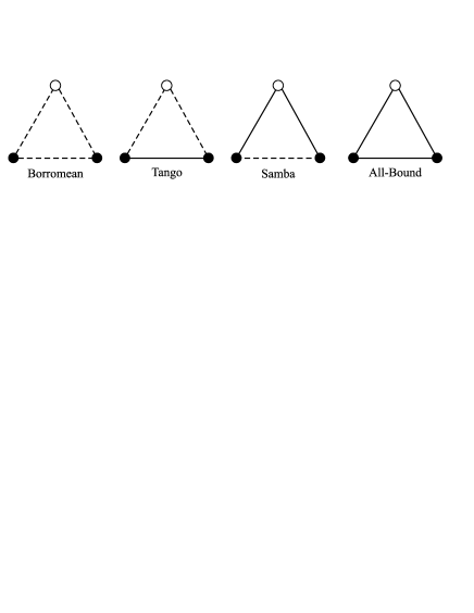
Figure 1: Diagrammatical representation of the classification scheme for weakly-bound three-body systems. Two-body bound state are represented with solid line, and virtual state with dashed line.

In the present work, we study the root-mean-square distances between the constituents of a bound three-body system, where we have two identical particles $n$ and a core named $A$. By $n$ we mean neutron in halo nuclei, but we allow the pair neutron-neutron ($nn$) to be bound in order to cover all the configurations presented above. We represent the radii in a scaling plot in terms of a dimensionless product, extending to halo nuclei a previous application that was done for molecules mol03 . Using these scaling plots we can follow the behavior of the different radii when it happens a transition between one kind of system to another one. Starting from the Borromean case (all unbound), we can go to the Samba case by increasing the binding energy of the pair $nA$ (keeping $nn$ unbound); and to the Tango case by increasing the binding energy of the pair $nn$ (keeping $nA$ unbound). In particular, we calculate the mean square distance between the two neutrons in ⁶He, ¹¹Li and ¹⁴Be (which have been measured recently marq00 ) from the known bound or virtual energies of the subsystems and the two-neutron separation energy.

The calculation of the scaling function for the different radii of the three-body system is performed with a renormalization scheme applied to three-body equations with $s-$wave zero-range pairwise potential, which makes use of subtracted equations ad95 ; yama02 .

As our approach is restricted to $s-$wave two-body interactions, some limitations in the application of our analysis are expected. The argument has the origin in the fact that, in some cases, the two-body subsystem interaction in $p-$wave is considered to be important for the three-body binding. The examples are ⁶He zheng93 , known to be bound by the $p-$wave interaction in $n-^{4}$He; and ¹¹Li, where both $p-$ and $s-$waves might be relevant to describe the ground state of the unbound subsystem ¹⁰Li (see discussion and references in caggi99 ). However, as pointed out in ref.zin95 (in a discussion related to ¹¹Li), one should also noticed that even the three-body wave function with $s-$wave $nn$ correlation produces a ground state of the halo nuclei with two or more shell-model configurations. The effect of the above $s-$wave restriction is also reduced due to the fact that we are considering the experimental energies in our approach, which implicitly are carrying the effect of higher partial waves in the interaction. Another aspect is that the radius are obtained from the tail of the wave-function, which is dominated by the $s-$wave.

The paper is organized as follows. In section II, we present our formalism, which contains the subtracted method to treat the Faddeev equations with two identical particles, leading to the form factors from which we obtain the different mean-square radii. We also give a brief discussion of the scaling functions to describe the radii. In section III, we discuss the classification scheme. In section IV, we present our numerical results for the root-mean-square distances between the particles. Our conclusions are summarized in section V.

II Formalism

In the next subsection, we consider the formalism given in refs. yama02 ; mol03 for coupled channels to calculate the three-body wave functions and the possible different radii with a zero-range pairwise interaction. We solve the homogeneous three-body Faddeev equations for a system with two identical particles $\alpha$ and a third one $\beta$ in a renormalized subtracted form, which allows one to obtain the observables as a function of the two and three-body scales of the system. The corresponding masses of the particles $\alpha$ and $\beta$ are $m_{\alpha}$ and $m_{\beta}$.

II.1 Subtracted Faddeev Equations

Next, we follow the model presented in refs. yama02 ; mol03 for the subtracted Faddeev equations, and consider units such that $\hbar=1$ and $m_{\alpha}=1$. For the subtraction energy that is required in the model, we choose $\mu_{(3)}^{2}$. In this case, all the energies and momentum variables are rescaled to dimensionless variables considering this subtraction energy. After partial wave projection, the $s-$wave coupled subtracted integral equations for the Faddeev spectator functions $\chi_{\alpha\alpha}$ and $\chi_{\alpha\beta}$, are given by:

$$\chi_{\alpha\alpha}(y) = 2\tau_{\alpha\alpha}(y;\epsilon_{3})\int_{0}^{\infty}dx\frac{x}{y}G_{1}(y,x;\epsilon_{3})\chi_{\alpha\beta}(x)$$ (1)

$$\chi_{\alpha\beta}(y) = \tau_{\alpha\beta}(y;\epsilon_{3})\int_{0}^{\infty}dx\frac{x}{y}\left[G_{1}(x,y;\epsilon_{3})\chi_{\alpha\alpha}(x)\right.$$ (2)

$$+ \left.AG_{2}(y,x;\epsilon_{3})\chi_{\alpha\beta}(x)\right],$$

$$\tau_{\alpha\alpha}(y;\epsilon_{3}) \equiv \frac{1}{\pi}\left[\sqrt{\epsilon_{3}+{\cal C}_{1}^{A}y^{2}}\mp\sqrt{\epsilon_{\alpha\alpha}}\right]^{-1},$$ (3)

$$\tau_{\alpha\beta}(y;\epsilon_{3}) \equiv \frac{1}{\pi}\frac{\left({\cal C}_{2}^{A}\right)^{3/2}}{\left[\sqrt{\epsilon_{3}+{\cal C}_{2}^{(A+1)}y^{2}}\mp\sqrt{\epsilon_{\alpha\beta}}\right]},$$ (4)

$$G_{1}(y,x;\epsilon_{3}) \equiv \log\frac{(\epsilon_{3}+x^{2}+xy)+{\cal C}_{2}^{A}\;y^{2}}{(\epsilon_{3}+x^{2}-xy)+{\cal C}_{2}^{A}\;y^{2}}$$ (5)

$$- \log\frac{(1+x^{2}+xy)+{\cal C}_{2}^{A}\;y^{2}}{(1+x^{2}-xy)+{\cal C}_{2}^{A}\;y^{2}},$$

$$G_{2}(y,x;\epsilon_{3}) \equiv \log\frac{(\epsilon_{3}+xy/A)+{\cal C}_{2}^{A}\;(y^{2}+x^{2})}{(\epsilon_{3}-xy/A)+{\cal C}_{2}^{A}\;(y^{2}+x^{2})}$$ (6)

$$- \log\frac{(1+xy/A)+{\cal C}_{2}^{A}\;(y^{2}+x^{2})}{(1-xy/A)+{\cal C}_{2}^{A}\;(y^{2}+x^{2})}~{},$$

where we are defining the mass ratio and the constant mass factors by

$$A\equiv\frac{m_{\beta}}{m_{\alpha}},\;\;\;\;{\cal C}_{j=1,2}^{A}\equiv\left(\frac{j}{4}+\frac{1}{2A}\right).$$ (7)

The plus and minus signs in eqs. (3) and (4) refer to virtual and bound two-body subsystems, respectively. In the equations above, the dimensionless three-body energy $\epsilon_{3}$ and the two-body energies ($\epsilon_{\alpha\alpha}$ and $\epsilon_{\alpha\beta}$), are related to the corresponding physical quantities by $\epsilon_{3}\equiv-E_{3}/\mu_{(3)}^{2},$ $\epsilon_{\alpha\alpha}\equiv-E_{\alpha\alpha}/\mu^{2}_{(3)},$ and $\epsilon_{\alpha\beta}\equiv-E_{\alpha\beta}/\mu^{2}_{(3)}.$ The three-body physical quantities can be written in terms of a scaling function, i.e., the dimensionless product of the observable and some power of the three-body binding energy $E_{3}$, when the value of $\mu^{2}_{(3)}$ is determined from the known value of $E_{3}$ and consequently the three-body quantities are naturally a function of $E_{3}$ and the ratios $E_{\alpha\alpha}/E_{3}$ and $E_{\alpha\beta}/E_{3}$. Note that we are using the same symbol $A$ for the mass ratio as well as for the core label, considering that, in a $n-n-$core nucleus we have the core consisting of $A$ nucleons and $A$ can also be identified with the mass ratio ($m_{\beta}=Am_{n}$, $m_{\alpha}=m_{n}$). However, our expression can be generally applied for non-integer values of $A$.

For large scattering lengths, the details of the interaction are unimportant to describe few-body systems, as the short-range informations, beyond the two-body scattering lengths, are carried out by one typical three-body scale. Therefore, the low-energy observables present a scaling behavior quite universal with the three-body binding energy fred87 ; ad95 . In the limit of infinite scattering lengths or zero range interactions, the function which represents a given correlation between two three-body observables, written in terms of scaled variables, converges to a single curve, despite the existence of many other Efimov states.

For a three-body system with binding energy $E_{3}$, in the scaling limit amorim97 ; yama02 , one general three-body physical observable $\cal O$, with dimension of energy to the power $\eta$, at a particular energy $E$, can be written as a function $\cal F$ of the ratios between the two and three-body energies, such that

$${\cal{O}}\left(E,E_{3},E_{\alpha\alpha},E_{\alpha\beta},\right)=$$

$$(E_{3})^{\eta}{\cal F}\left(\sqrt{\frac{E}{E_{3}}},\pm\sqrt{\frac{E_{\alpha\alpha}}{E_{3}}},\pm\sqrt{\frac{E_{\alpha\beta}}{E_{3}}},A\right)\ .$$ (8)

The two-body energies $E_{\alpha\gamma}$ ($\gamma=\alpha,\;\beta$), are negative quantities, corresponding to bound or virtual states. The nature of such two-body state, bound or virtual, is revealed in the momentum space, such that we have a bound state when $\sqrt{|E_{\alpha\beta}|}$ is positive and a virtual state when $\sqrt{|E_{\alpha\beta}|}$ is negative. So, in equation (8), the signs $+$ or $-$ mean a bound or virtual two-body subsystem, respectively. The different radii of the bound $\alpha\alpha\beta$ system are functions defined from the eq. (8) with $E=E_{3}$, which depend on the mass ratio, $A$, the ratios of the two and three-body energies and the kind of subsystem interactions (bound or virtual).

II.2 Radii calculation

The Faddeev components of the wave-function for the $\alpha\alpha\beta$ system are written in terms of the spectator functions, obtained from the solution of eqs. (1) and (2) in momentum space:

$$\Psi_{\alpha\alpha}(\vec{y},\vec{z})=\left(\frac{1}{\epsilon_{3}+{\cal C}_{1}^{A}\;\vec{y}^{2}+\vec{z}^{2}}-\frac{1}{1+{\cal C}_{1}^{A}\;\vec{y}^{2}+\vec{z}^{2}}\right)$$

$$\times\left[\chi_{\alpha\alpha}(|\vec{y}|)+\chi_{\alpha\beta}\left(\left|\vec{z}-\frac{\vec{y}}{2}\right|\right)+\chi_{\alpha\beta}\left(\left|\vec{z}+\frac{\vec{y}}{2}\right|\right)\right],$$

(9)

$$\Psi_{\alpha\beta}(\vec{y},\vec{z})=$$

$$\left(\frac{1}{\epsilon_{3}+{\cal C}_{2}^{A}\;\vec{z}^{2}+{\cal C}_{2}^{A+1}\;\vec{y}^{2}}-\frac{1}{1+{\cal C}_{2}^{A}\;\vec{z}^{2}+{\cal C}_{2}^{A+1}\;\vec{y}^{2}}\right)$$

$$\times\left[\chi_{\alpha\alpha}\left(\left|\vec{z}-\frac{A\vec{y}}{A+1}\right|\right)+\chi_{\alpha\beta}(|\vec{y}|)+\chi_{\alpha\beta}\left(\left|\vec{z}+\frac{\vec{y}}{A+1}\right|\right)\right],$$

where ${\cal C}_{j}^{A}$ is defined in eq. (7). The Faddeev components are denoted by the sub-indices of the interacting pair. Representing the pair by $\alpha\gamma$ with $\gamma\ =\ \alpha$ or $\beta$, one has that $\vec{z}$ is the relative momentum between $\alpha$ and $\gamma$ and $\vec{y}$ is the relative momentum of the third particle to the center-of-mass of the system $\alpha\gamma$. For the halo nuclei the notation is $\alpha~{}=~{}n$ and $\beta$ is the core represented by $A$.

The momentum component of the total wave-function,

$$\Psi_{Ann^{\prime}}=\Psi_{nn^{\prime}}+\Psi_{An}+\Psi_{An^{\prime}}~{},$$ (10)

is symmetrical by the exchange between the neutrons, $n$ and $n^{\prime}$, while the antisymmetry is given by the singlet spin-component (not explicitly shown). The different mean-square radii are calculated from the derivative of the Fourier transform of the respective matter density in respect to the square of the momentum transfer. The relative mean-square distances between the halo neutrons and between the neutron and the core ($\gamma~{}=n,A$) are obtained from the expression

$$\langle r^{2}_{n\gamma}\rangle=-6\frac{dF_{n\gamma}(q^{2})}{dq^{2}}\bigg{|}_{q^{2}=0},$$ (11)

where

$$F_{n\gamma}(q^{2})=\int\;d^{3}y\;d^{3}z\Psi_{Ann^{\prime}}\left(\vec{y},\vec{z}+\frac{\vec{q}}{2}\right)\;\Psi_{Ann^{\prime}}\left(\vec{y},\vec{z}-\frac{\vec{q}}{2}\right)$$ (12)

is the Fourier transform of the two-body densities, which is a function of the momentum transfer $\vec{q}$ (given in units of $\mu_{(3)}$). The relative momentum between $n$ and $\gamma$ is $\vec{z}\pm\vec{q}/2$ and the relative momentum of the third particle to the center-of-mass of $n\gamma$ is $\vec{y}$.

Analogous equations can be found for the mean square distances of the neutron and the core to the center-of-mass system ($\langle r^{2}\rangle_{\gamma}$), in terms of the Fourier transform of the one-body density.

II.3 Scaling functions for the radii

The scaling functions for the mean-square separation distances between the particles in the three-body system can be written according to eq.(8) with $E\equiv E_{3}$. The scaling functions for the radii are written as:

$$\sqrt{\langle r^{2}_{n\gamma}\rangle|E_{3}|}={\cal R}_{n\gamma}\left(\pm\sqrt{\frac{E_{nn}}{E_{3}}},\pm\sqrt{\frac{E_{nA}}{E_{3}}},A\right),$$ (13)

$$\sqrt{\langle r^{2}_{\gamma}\rangle|E_{3}|}={\cal R}_{\gamma}^{cm}\left(\pm\sqrt{\frac{E_{nn}}{E_{3}}},\pm\sqrt{\frac{E_{nA}}{E_{3}}},A\right).$$ (14)

To study the different types of three-body systems, the general scaling function for the radii given by eqs. (13) and (14) will be studied in the configurations of figure 1. However, one noticeable situation occurs when the Efimov limit is reached, for which the subsystems energies vanishes, and

$$\sqrt{\langle r^{2}_{n\gamma}\rangle|E_{3}|}={\cal R}_{n\gamma}\left(A\right),~{}~{}\sqrt{\langle r^{2}_{\gamma}\rangle|E_{3}|}={\cal R}_{\gamma}^{cm}\left(A\right),$$ (15)

depends only on the mass ratio $A$ $(\gamma=n,A)$. Curiously, this configuration contains simultaneously all types shown in figure 1.

III Classification Scheme: qualitative properties

A discussion of a classification scheme for a bound three-body system, with two identical particles, is given in ref. jensen03 , according to the nature of the subsystem interactions, which can present a bound or virtual state, as depicted diagrammatically in figure 1.

The different possibilities of three-body systems are reflected in the qualitative properties of the dynamics as given by the coupled equations (1) and (2) in terms of the strength of the attractive kernel of these equations. Let us describe all these possibilities. The Borromean case corresponds to positive signs in front of the square-root of the energies of the subsystems in both eqs. (3) and (4). A Tango three-body system has a negative sign only in front of $\sqrt{\epsilon_{\alpha\alpha}}$ in eq. (3), with positive sign in front of $\sqrt{\epsilon_{\alpha\beta}}$ in eq. (4). For a Samba configuration of the three-body system, a minus sign appears multiplying $\sqrt{\epsilon_{\alpha\beta}}$ in eq. (4), while a plus sign multiplies $\sqrt{\epsilon_{\alpha\alpha}}$ in eq. (3). The All-Bound system has negative signs in eqs.(3) and (4). As a consequence of the differences in eqs.(3) and (4), the weakest attractive kernel in eqs.(1) and (2) is given by a Borromean three-body system, followed by the Tango, Samba and All-Bound systems. Therefore, once fixed a three-body binding energy, the system for which the kernel presents the weakest attraction will have the smallest configuration. So, the size of the corresponding system will increase in the following order: Borromean, Tango, Samba and All-Bound. The All-Bound configuration has the biggest size among all, for a given three-body binding energy. One of course has to remind that the sizes are expected to increase when the binding energy hits one scattering threshold. Therefore, for nonvanishing three-body binding energy this situation does not happen only in the Borromean case. In this sense, it is physically sensible that the Borromean case corresponds to the smallest configuration size. This observation will be explored in our numerical calculations. In this respect, we are showing the quantitative detailed implication to the different radii of weakly-bound three-body systems of the classification scheme proposed in ref. jensen03 .

IV Numerical Results for the radii: scaling plots

We present numerical results for the different possible radii for Borromean, Tango, Samba and All-Bound three-body configurations obtained from the wave-function, eq. (10) derived from the solution of eqs. (1) and (2). In particular, we give results for the neutron-neutron ($nn$) average distance in the three-body halo nuclei, ⁶He, ¹¹Li, ¹⁴Be, ²⁰C.

It is interesting to present results in a general scaled form in terms of scaled two-body binding energies and mass ratio, as given by eqs. (13) and (14), which turns to be useful for the prediction of the several radii in different situations for weakly bound molecules up to light halo-nuclei. Our calculations present results independent on the detailed form of the interactions in a weakly bound three-body system. It means that they apply very well to halo nuclei and weakly bound molecules. The present approach is valid as long as the interactions within the three-body system are of short range while the two-body energies are close to zero, i.e., the ratio between the interaction range and the modulus of the scattering lengths should be somewhat less than 1. These are indeed the cases we are considering. We present results only for the ground state of the three-body system. We have shown that the scaling function for the radii is indeed approached even for a calculation of the ground state in our subtraction scheme mol03 , which will be enough for our purpose.

Figure 2: Dimensionless products $\sqrt{\langle r^{2}_{n\gamma}\rangle|E_{3}|}$ and $\sqrt{\langle r^{2}_{\gamma}\rangle|E_{3}|}$ $(\gamma=n,A)$ as a function of $A$ for zero two-body energies. Results for: (a) $\sqrt{\langle r^{2}_{nn}\rangle|E_{3}|}$ (upper solid line) and $\sqrt{\langle r^{2}_{nA}\rangle|E_{3}|}$ (upper dot-dashed line); (b) $\sqrt{\langle r^{2}_{n}\rangle|E_{3}|}$ (lower solid curve) and $\sqrt{\langle r^{2}_{A}\rangle|E_{3}|}$ (lower dot-dashed curve). The experimental data, obtained from marq00 , are for $\sqrt{\langle r^{2}_{nn}\rangle|E_{3}|}$.

In figure 2, we show the results of the scaling function for the mean square distances, $\sqrt{\langle r^{2}_{n\gamma}\rangle}$ and $\sqrt{\langle r^{2}_{\gamma}\rangle}$ with $\gamma=~{}n$ or $A$ (see eq. (15)) which are shown as a function of $A$ for $E_{n\gamma}=0$. The comparison with experimental results of $\sqrt{\langle r^{2}_{nn}\rangle}$ marq00 , for the ⁶He, ¹⁴Be and ¹¹Li is just for illustrative purpose, considering the hypothetical cases that ⁵He, ¹³Be and ¹⁰Li would have virtual states close to zero energy. Such hypothesis is more realistic in case of ¹⁴Be, while for the ⁶He and ¹¹Li are not so. As shown by our results for ¹¹Li, given in Table I, the assumption of a virtual state with energy close to zero ($|E_{nA}|\lesssim$0.05 MeV zin95 ) for ¹⁰Li lead to an average $nn$ separation distance (in the halo of ¹¹Li) not compatible with the corresponding experimental result. Given that it is well documented the difficulty in studying the ¹⁰Li caggi99 , we can consider $\sqrt{\langle r^{2}_{nn}\rangle}$ marq00 as one of our inputs to predict the virtual state of the $n-^{9}$Li system. In this case, we conclude that it cannot be smaller than $\sim$ 0.1 MeV.

In this case ($E_{n\gamma}=0$) the only physical scale is $E_{3}$ and the scaling plots will depend solely on $A$. The average separation distance between the neutrons and the neutron-core tends naturally to a constant for large $A$, while it diverges for $A$ tending towards zero. The reason for the unbound increase of the products $\langle r^{2}_{nn}\rangle|E_{3}|$ and $\langle r^{2}_{nA}\rangle|E_{3}|$ for small $A$ is due to the average momentum of the core which tends to zero ($\sim\sqrt{A|E_{3}|}$) extending the system to infinity. We have checked that the results shown in figure 2 tends to finite values after multiplication by $\sqrt{A}$ (one has to remember that we are using units of $m_{n}=1$).

The average distance of the neutron to the center of mass system tends to become the relative distance to the core, when the core mass grows to infinity. This fact is clearly seen in figure 2 with the lower solid line approaching the upper dot-dashed one when $A\gtrsim 10$. Also, one sees that the core distance to the center of mass vanishes with growing $A$ as it should be.

Table 1: Results of the neutron-neutron root-mean-square radii in halo nuclei. The cores ($A$) are given in the first column, the absolute values of the three-body ground state energies $E_{3}$ are given in the second column. For $-E_{3}$, which is equal to the two-neutron separation energy $S(2n)$, we consider the center value of the corresponding energies given in ref. audi95 , except for Lithium. In case of Lithium we consider for $-E_{3}$ the maximum (0.32 MeV) and the center value (0.29 MeV) given in ref. tan96 . In the third column we give our input values for $-E_{nA}$, considering several values, covering the values suggested in the literature (the references are given together with the corresponding number). For bound two-body subsystem $nA$, we have $-E_{nA}$ equal to the one-neutron separation energy $S(n)$. The virtual states are indicated by (v), and the $nn$ virtual state energy is taken as -143 keV. The experimental values, in the last column, are obtained from Marqués et al. (2000)marq00 .

Core	$-E_{3}$	$-E_{nA}$		$\sqrt{\langle r_{nn}^{2}\rangle}$	$\sqrt{\langle r_{nn}^{2}\rangle}_{exp}$
(A)	(MeV)	(MeV)		(fm)	(fm)
		0	(v)	5.1
4He	0.973	0.3	(v)	4.6	5.9$\pm$1.2
		4.0 aj88	(v)	3.6
9Li	0.32	0	(v)	9.2	6.6$\pm$1.5
		0.8 wil75	(v)	5.9
		0	(v)	9.7
9Li	0.29	0.05 zin95 ; bar01 ; tho99	(v)	8.5	6.6$\pm$1.5
		0.8 wil75	(v)	6.7
12Be	1.337	0	(v)	4.6	5.4$\pm$1.0
		0.2tho00	(v)	4.2
18C	3.50	0.16audi95		3.0	-
		0.53naka99		4.4	-

Figure 3: Dimensionless products $\sqrt{\langle r^{2}_{nA}\rangle|E_{3}|}$ (upper frame) and $\sqrt{\langle r^{2}_{nn}\rangle|E_{3}|}$ (lower frame) for $A=0.1$ and $E_{nn}/E_{3}=K_{nn}^{2}=0.1$ as a function of ${K_{nA}/|K_{nn}|}$. In the upper frame, a bound $nn$ pair is represented with dashed line; and a virtual $nn$ pair with dot-dashed line. In the lower frame, a bound $nn$ pair is represented with solid line; and a virtual $nn$ pair with dotted line. The transition between the configurations occurs when $K_{nA}=0$ (represented by the vertical line).

Figure 4: Dimensionless products $\sqrt{\langle r^{2}_{nA}\rangle|E_{3}|}$ (upper frame) and $\sqrt{\langle r^{2}_{nn}\rangle|E_{3}|}$ (lower frame) for $A=1$ and $K_{nn}^{2}=0.1$ as a function of ${K_{nA}/|K_{nn}|}$. The convention of the lines is the same as given in figure 3.

Figure 5: Dimensionless products $\sqrt{\langle r^{2}_{nA}\rangle|E_{3}|}$ (upper frame) and $\sqrt{\langle r^{2}_{nn}\rangle|E_{3}|}$ (lower frame) for $A=200$ and $E_{nn}/E_{3}=0.1$ as a function of ${K_{nA}/|K_{nn}|}$. The convention of the lines is the same as given in figures 3 and 4.

Figure 6: Dimensionless products $\sqrt{\langle r^{2}_{nA}\rangle|E_{3}|}$ (upper frame) and $\sqrt{\langle r^{2}_{nn}\rangle|E_{3}|}$ (lower frame) for $A=200$ and $E_{nA}/E_{3}=0.1$ as a function of ${K_{nn}/|K_{nA}|}$. In the upper we represent the case of a bound $nA$ pair with dashed line; and the case of a virtual $nA$ pair with dot-dashed line. In the lower frame we represent the bound $nA$ pair with solid line and the virtual $nA$ pair with dotted line. The lines of this figure correspond to the vertical transitions represented in figure 5 in both extreme sides where $|K_{nA}|=|K_{nn}|$.

In the figures 3 to 6, we show results for $\sqrt{\langle r^{2}_{nn}\rangle|E_{3}|}$ and $\sqrt{\langle r^{2}_{nA}\rangle|E_{3}|}$, when one of the subsystem energies is fixed in respect to the three-body binding energy, while the other one varies. We use values of $A$ equal to 0.1, 1 and 200. The subsystems can be bound or virtual and therefore all configurations are covered, i.e., we show results for Borromean, Tango, Samba and All-bound-type systems. Anticipating the presentation of these figures, in general we find that, the radii increase in the following order Borromean, Tango, Samba and All-bound for a given three-body energy and fixed $A$. In our analysis below, we fix either $E_{nn}/E_{3}=0.1$ or $E_{nA}/E_{3}=0.1$ which can correspond to bound or virtual subsystem energies. In the next, we also consider the definitions $E_{nA}/E_{3}\equiv K^{2}_{nA}$ and $E_{nn}/E_{3}\equiv K^{2}_{nn}$ (for both bound or virtual-state energies), such that

$$K_{nA}=\pm\sqrt{E_{nA}/E_{3}}\;\;\;\;{\rm and}\;\;\;K_{nn}=\pm\sqrt{E_{nn}/E_{3}}.$$ (16)

The $+(-)$ sign refers to bound(virtual) state. One should also note that, the dimensionless quantities $K_{nn}$ and $K_{nA}$ are directly related to poles in the imaginary axis of the respective two-body momentum space.

In figure 3, we present calculations of the $nA$ and $nn$ root-mean-square radius as functions of $K_{nA}/|K_{nn}|$. Such average radius, multiplied by $\sqrt{|E_{3}|}$, are scaled to dimensionless quantities. We consider $A=0.1$ and $E_{nn}/E_{3}=0.1$ fixed, corresponding to bound ($K_{nn}=\sqrt{0.1}$) or virtual ($K_{nn}=-\sqrt{0.1}$) subsystems. In this case, the mass of the particle $n$ is much heavier than the “core”, which does not happen in halo nuclei. However, we consider this case for the sake of general interest. In the $x-$axis, the positive (negative) values of $K_{nA}/|K_{nn}|$ correspond to bound (virtual) $nA$ states. In the upper frame, the average $nA$ radius is shown for a bound $nn$ pair (dashed line) and for a virtual $nn$ pair (dot-dashed line). So, the dashed line shows that the value of $\sqrt{\langle r^{2}_{nA}\rangle|E_{3}|}$ increases with the transition from Tango to All-bound configuration. In the other possibility, represented by the dot-dashed line ($nn$ in a virtual state), the value of $\sqrt{\langle r^{2}_{nA}\rangle|E_{3}|}$ increases from the most compact Borromean configuration ($K_{nA}$ negative) to the Samba-type configuration ($K_{nA}$ positive).

In the lower frame of figure 3, we also show that $\sqrt{\langle r^{2}_{nn}\rangle|E_{3}|}$ increases with the transition from Tango to All-bound and Borromean to Samba configurations. We observe, in this case, a small sensitivity on $K_{nn}$, when going from $-\sqrt{0.1}$ (dotted line) to $\sqrt{0.1}$ (solid line), with $\sqrt{\langle r^{2}_{nn}\rangle|E_{3}|}$ having practically the same value for the All-bound and Samba configurations; and also for the Tango and Borromean configurations. As we increase $A$, this sensitivity increases, as one can see in the next figures 4 and 5. We interpret this as the dominant role played by a light particle in the long-range interaction between two heavy particles, $n$, as already shown in an adiabatical approximation of the three-body system fonseca79 .

In figure 4, we show the radii for the ground state of the three-body system with the mass ratio $A=1$. As in figure 3, we fixed $K_{nn}=\pm\sqrt{0.1}$, corresponding to bound ($+$) or virtual ($-$) subsystems. The same behavior found in figure 3 for $\sqrt{\langle r^{2}_{nA}\rangle|E_{3}|}$ is found in the upper frame of figure 4 for $A=1$, i.e., the configurations for which the $nn$ pair is virtual (dot-dashed line) are smaller than the ones that have the $nn$ pair bound (dashed line). Besides that, the configuration increases in size when the system changes from a Borromean to a Samba type and when it changes from a Tango to an All-bound type. For $A=1$, the mean square distance between the two-neutrons (lower frame of figure 4) exhibits the same qualitative behavior as found for $\sqrt{\langle r^{2}_{nA}\rangle|E_{3}|}$ when the configuration type is modified for a fixed three-body energy. These conclusions are still valid for a heavy core particle with $A=200$, as one can verify in figure 5. It is worthwhile to mention that $\sqrt{\langle r^{2}_{nn}\rangle|E_{3}|}$ attains its asymptotic value fast with the increase of $A$ consistently with the calculations presented in figure 2 for $E_{nn}=E_{nA}=0$. (Compare the results for $A=1$ and $A=200$ in the lower frames of figures 4 and 5).

In correspondence with figure 5, for the same mass ratio $A=200$, in the last set of systematic calculations we consider in figure 6 the energy of the subsystem $nA$ fixed in relation to $E_{3}$, with $K_{nA}=\pm\sqrt{0.1}$, corresponding to bound ($+$) or virtual ($-$) $nA$ subsystem. In this case, the ratio $K_{nn}/|K_{nA}|$ is changed from $-1$ to $+1$, such that the transitions of configurations from the left side to the right side of this figure correspond to the vertical transitions in the extreme side of figure 5 (when $|K_{nA}|=|K_{nn}|=\sqrt{0.1}$). So, comparing the upper frames of figures 5 and 6, we observe that the vertical transition from All-bound to Samba configuration in figure 5 corresponds to the dashed line of figure 6; and, the vertical transition from Tango to Borromean configuration in figure 5 corresponds to the dot-dashed line of figure 6. In the lower frames of both figures, similarly we observe that the vertical transitions of figure 5 correspond to the lines represented in figure 6: the transition from Samba to All-bound configuration is given by the solid line; and the transition from Borromean to Tango configuration given by the dotted line. In general, one can observe that the three-body bound state has a smaller size when the $nA$ pair forms a virtual state (see in each frame of figure 6, where the upper line is for bound and the lower line is for virtual $nA$ pair).

The calculations of the average distances of the neutrons in the halo of ⁶He, ¹¹Li, ¹⁴Be and ²⁰C are shown in Table I and compared with the available experimental data. For the input, we have considered $E_{nn}=-0.143$ MeV and the center of the available experimental values of $E_{3}$ and $E_{nA}$. For the cases that we have unbound virtual $nA$ systems, the $E_{nA}$ input values are taken from several recent theoretical and experimental analysis; we prefer to keep at least two possible values in order to verify the consistency of the model with the experimental data.

Within the possible limitations of our approach, by comparing our results for the $nn$ mean-square radius with the experimental ones, which are known in the cases of ⁶He, ¹¹Li and ¹⁴Be, as given in Table 1, one can also predict the corresponding virtual energies of the $nA$ subsystem.

In the particular case of ⁶He, the comparison between the experimental $nn$ mean-square radius with our result is pointing out to a virtual energy close to zero for $n-^{4}$He, which is not supported by the quite large values given in the literature zheng93 ; aj88 . However, as discussed in zheng93 ; aj88 , the interaction for $n-^{4}$He is attractive in $p-$wave and repulsive in $s-$wave producing a large value for the energy of the virtual state, such that a deviation of our calculation from the experimental result is expected (in our model the $s-$wave poles should be near the scattering thresholds). For the binding of ¹¹Li, it is also known that both $p-$ and $s-$waves are important in the subsystem $n-^{9}$Li. This fact can also explain some deviations of our results when compared with experimental ones. However, in this last case, our approach can be more reliable based on the fact that: (i) the $s-$wave $n-^{9}$Li interaction is attractive and it has a virtual state near the scattering region; (ii) we are considering the experimental energies for the inputs, such that we are partially taking into account the effect of higher partial waves in the interactions; (iii) the radius is obtained from the tail of the wave-function, which is dominated by the $s-$wave; (iv) as noted in ref. zin95 , even the three-body wave function with $s-$wave $nn$ correlation produces a ground state of the halo nuclei with two or more shell-model configurations.

One should also expect that other effects like the finite size of the core and Pauli principle, missing in our model, could affect the average relative distances, if the three-body wave function would overlap appreciably with the core. At least for ¹¹Li this is not expected due to the small binding. It is of notice that indeed the halo neutrons have a large probability to be in a region in which the wave function is an eigenstate of the free Hamiltonian, and thus dominated by few asymptotic scales.

V Conclusions

The mean-square radii of a light halo-nuclei modelled as a three-body system (two neutrons $n$ and a core $A$) are calculated using a renormalized three-body model with a pairwise Dirac-$\delta$ interaction, which works with a minimal number of physical inputs directly related to observables. These physical scales are the two-neutron separation energy $S(2n)=-E_{3}$, and the $nn$ and $n-$core $s-$wave scattering lengths.

The existent data for ¹¹Li and ¹⁴Be compare qualitatively well with our theoretical results, which means that the neutrons of the halo have a large probability to be found outside the interaction range. Therefore the low-energy properties of these halo neutrons are, to a large extend, model independent as long as few physical input scales are fixed. The model provides a good insight into the three-body structure of halo nuclei, even considering some of its limitations. We pointed out that the model is restricted to $s-$wave subsystems, with small energies for the bound or virtual states. So, the model is not suitable for the ⁶He, since the $s-$wave virtual state energy of ⁵He is quite large (-4 MeV). There is no $n-$core $p-$wave interaction, although some of its physics is effectively included through the value of the two-neutron separation energy, which is an input for our radii calculations. Also the finite size of the core and consequently the antisymmetrization of the total nuclear wave function, are both missing in our model. However, as the three-body halo nuclei tend to be more and more weakly bound with subsystems that have bound or virtual states near the scattering threshold, our approach becomes adequated and the above limitations are softened. The results indicate that the model is reasonable for ¹¹Li and ¹⁴Be.

As an example of application to other halo-nuclei system, considering the available energies, we have also estimated the $nn$ root-mean-square radius for the $n-n-^{18}$C system.

We have also studied in detail the consequences of the classification scheme proposed in Ref. jensen03 for weakly bound three-body systems. This study was performed analyzing the dimensionless products $\sqrt{\langle r^{2}_{nA}\rangle|E_{3}|}$ and $\sqrt{\langle r^{2}_{nn}\rangle|E_{3}|}$ in terms of scaling functions depending on the dimensionless product of the scattering lengths and the square-root of the neutron-neutron separation energy. In the cases we have addressed, there are four different types of a three-body system when we allow the neutron-neutron pair to be bound: Borromean (only virtual two-body subsystems), Tango ($nn$ bound and $nA$ virtual), Samba ($nn$ virtual and $nA$ bound) and All-Bound (only bound two-body subsystems). The name Samba was introduced to refer to a system quite stable because it has two bound two-body subsystem than the Tango type, so it can “shake” a little bit more and continue to be bound.

The qualitative properties of the different possibilities of three-body systems are easily understood in terms of the effective attraction in the model: when a pair has a virtual state the effective interaction is weaker than when the pair is bound. Thus, a three-body system has to shrink to keep the binding energy unchanged if a pair which is bound turns to be virtual. We have illustrated through several examples this property, which show that dimensionless sizes $\sqrt{\langle r^{2}_{nA}\rangle|E_{3}|}$ and $\sqrt{\langle r^{2}_{nn}\rangle|E_{3}|}$ increase from Borromean, Tango, Samba and to All-Bound configurations. Of course the size is expected to increase beyond limits when a nonvanishing three-body energy hits a scattering threshold, with the Borromean configuration being the only exception. In spite of that, we conclude that even far from the threshold situation, the configuration sizes increase as we pointed out.

We would like to thank Fundação de Amparo à Pesquisa do Estado de São Paulo (FAPESP) for partial support. LT and TF also thank partial support from Conselho Nacional de Desenvolvimento Científico e Tecnológico (CNPq).

References

- (1) M.V. Zhukov, B.V. Danilin, D.V. Fedorov, J.M. Bang, I.J. Thompson, J.S. Vaagen, Phys. Rep. 231 (1993) 151.
- (2) E. Nielsen, D.V. Fedorov, A.S. Jensen and E. Garrido, Phys. Rep. 347 (2001) 373.
- (3) G. Audi and A.H. Wapstra, Nucl. Phys. A 595 (1995) 409.
- (4) A.E.A. Amorim, L. Tomio and T. Frederico, Phys. Rev. C 56 (1997) R2378.
- (5) Efimov, V.: Phys. Lett. B 33 (1970) 563.
- (6) D. V. Fedorov, A. S. Jensen, and K. Riisager Phys. Rev. Lett. 73 (1994) 2817.
- (7) I. Mazumdar, V. Arora, and V. S. Bhasin Phys. Rev. C 61 (2000) 051303.
- (8) S.K. Adhikari, T. Frederico and I.D. Goldman, Phys. Rev. Lett. 74 (1995) 487; S.K. Adhikari and T. Frederico, Phys. Rev. Lett. 74 (1995) 4572.
- (9) T. Frederico, L. Tomio, A. Delfino, and A. E. A. Amorim, Phys. Rev. A 60 (1999) R9.
- (10) S. K. Adhikari, A. Delfino, T. Frederico, I. D. Goldman, and L.Tomio, Phys. Rev. A 37 (1988) 3666.
- (11) M.T. Yamashita, T. Frederico, R.S. Marques de Carvalho, and L. Tomio, Radii of weakly bound three-body systems: halo nuclei and molecules, nucl-th/0308072, to appear in Nucl. Phys. A.
- (12) A.S. Jensen, K. Riisager, D.V. Fedorov and E. Garrido, Europhys. Lett. 61 (2003) 320.
- (13) F. Robicheaux, Phys. Rev. A 60 (1999) 1706.
- (14) T. Nakamura et al., Phys. Rev. Lett. 83 (1999) 1112.
- (15) M.T. Yamashita, R.S. Marques de Carvalho, L. Tomio and T. Frederico, Phys. Rev. A 68 (2003) 012506.
- (16) F.M. Marqués et al., Phys. Lett. B 476 (2000) 219; Phys. Rev. C 64 (2001) 061301.
- (17) M.T. Yamashita, T. Frederico, A. Delfino, and L. Tomio, Phys. Rev. A 66 (2002) 052702.
- (18) D.C. Zheng et al., Phys. Rev. C 48 (1993) 1083.
- (19) J.A. Caggiano et al., Phys. Rev. C 60 (1999) 064322.
- (20) M. Zinser et al., Phys. Rev. Lett. 75 (1995) 1719; M. Zinser et al., Nucl. Phys. A 619 (1997) 151.
- (21) T. Frederico, I. D. Goldman, Phys. Rev. C 36 (1987) R1661.
- (22) I. Tanihata, J. Phys. G22 (1996) 157.
- (23) F. Ajzenberg-Selove, Nucl. Phys. A490 (1988) 1.
- (24) K.H. Wilcox et al., Phys. Lett. 59B (1975) 142.
- (25) F. Barranco, P.F. Bortignon, R.A. Broglia, G. Colo, E. Vigezzi, Eur. Phys. J. A 11 (2001) 385.
- (26) M. Thoennessen et al. Phys. Rev. C 59 (1999) 111.
- (27) M. Thoennessen, S. Yokoyama, P.G. Hansen, Phys. Rev. C 63 (2000) 014308.
- (28) A. C. Fonseca, E. F. Redish and P. E. Shanley, Nucl. Phys. A 320 (1979) 273.