Quasi-elastic knockout of pions and kaons from nucleons by high-energy electrons and quark microscopy of “soft” meson degrees of freedom in the nucleon

Abstract

Electro-production of pions and kaons at the kinematics of quasi-elastic knockout (which is well known in the physics of atomic nucleus and corresponds to the $t$-pole diagram) is proposed for obtaining their momentum distribution (MD) in various channels of virtual decay $N\to B+\pi$, $B=N$, $\Delta$, $N^{*}$, $N^{**}$, and $N\to Y+K$, $Y=\Lambda$, $\Sigma$. It is a powerful tool for investigation of a quark microscopic picture of the meson cloud in the nucleon. A model of scalar $q\bar{q}$ (${}^{3}P_{0}$) fluctuation in the non-trivial QCD vacuum is used to calculate pion and kaon momentum distributions (MD) in these channels.

1 Introduction

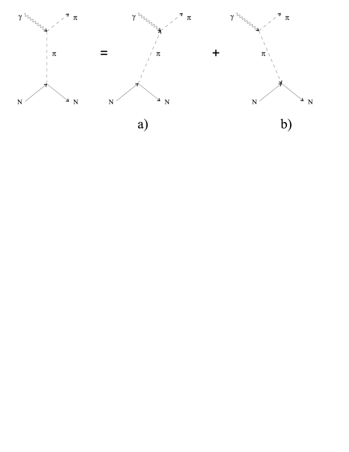
Figure 1: Feynman $t$-pole diagram for the pion production off the nucleon: a) the quasi-elastic knockout of pion; b) $z$-diagram of $\pi^{+}\pi^{-}$ production.

Investigation of structure of a composite system by means of quasi-elastic knockout of its constituents has been playing a very important role in the micro-physics [1, 2, 3, 4, 5, 6]. In a broad sense, the term ”quasi-elastic knockout” means that a high-energy projectile (electron, proton, etc.) instantaneously knocks out a constituent — an electron from an atom, molecule or solid film [1, 2], a nucleon [3] or cluster [4] from a nucleus, a meson from a nucleon [5] or nucleus [6] — transferring a high momentum in an ”almost free” binary collision to the knocked-out particle and leading to controllable changes in the internal state of the target. Such process corresponds to the Feynman pole diagram Fig. 1.

Exclusive quasi-elastic knockout coincidence experiments resolve individual states of the final system (different channels of the virtual decay of the initial composite system into a constituent and a final system-spectator in a given excited state). First of all, such experiments, in accordance with the laws of binary collisions [2], give the missing momentum and energy, i.e. the momentum of the constituent and its binding energy in the channel being considered. Of course, these values should be much smaller than momentum and energy of the final knocked-out particle. By varying kinematics, one can directly measure the momentum distribution (MD) of a constituent in different channels. For example, in the case of nuclei, such experiments make it possible to determine the momentum distributions of nucleons in different nuclear shells. Second, in such experiments, it is possible to measure spectroscopic factors of constituent separation in various channels. For nuclei, the spectroscopic factors determine probabilities of exciting different states of the residual nucleus-spectator $A-1$ after the knockout of a nucleon from the initial nucleus $A$ (it corresponds to the spectrum of relevant fractional-parentage coefficients [7], used in the theory of many-particle nuclear shell model).

In the present paper, we discuss a problem of how the above-mentioned experience can be extended to the investigation of a quark microscopic picture of meson cloud in the nucleon. We investigate here a pion production on nucleons by electrons with energy of a few GeV within the kinematics of quasi-elastic knockout. We rely on both the corresponding international literature [8, 9] and our previous results [5, 10].

Our relativistic analysis is done within the instantaneous form of dynamics in the initial proton rest frame (laboratory frame) as far as the kinematics criterion of the quasi-elastic character of the process (a large momentum of the knocked-out particle and a small recoil momentum of the residual system-spectator) is especially distinct here. If this reference frame is accepted, a significant contribution from the pole $Z$-diagram (Fig. 1b) should be taken into account, too. The corresponding amplitude may easily be obtained from the amplitude of the diagram Fig.1a using the crossing symmetry relations [11].

Within the quasi-elastic knockout kinematics (which includes the condition $Q^{2}\sim$ 1-3 (GeV/$c$)², $q^{\mu}q_{\mu}=-Q^{2}$ being the 4-momentum squared of the virtual photon) the pole mechanisms of Fig. 1a and Fig. 1b dominate [10]. The physical attractiveness of such kinematics in the quasifree collision can be illustrated, in particular, by the fact, that the problem of the gauge invariance of the knockout process is reduced here to that for the two-body electron-meson free collision, i.e. to the solved problem (see formal comments below and in Refs. [5, 10]). The authors of a preceding pioneering papers [8, 9] have analyzed an exclusive pion electro-production experiment $p(e,e^{\prime}\pi^{+})n$ [12, 13, 14] with $Q^{2}$ values ranging from 0.7 to 3.3 (GeV/$c$)² within the pole approximation and have reconstructed the MD of pions in the channel $p\to n+\pi^{+}$. But the problem of how much non-pole diagrams are suppressed here and how to make this suppression maximal by varying kinematics was not discussed.

In Refs. [8, 9], the light-front dynamics was used and the MDs were expressed in terms of ($x$, $k_{\perp}$) variables. This approach may be very helpful in more complicated cases (the interference of many different diagrams) as far as the contributions of all $z$-diagrams disappear here, but for our simplest situation of two pole amplitudes with the common vertex function such approach is not indispensable.

Further, papers [9, 10] contain an important note that while for pion photo-production reactions ($Q^{2}=0$) contributions of the $t$-pole and $s$-pole diagrams are compatible, for the pion electroproduction the relative contribution of non-$t$-pole diagrams decreases with increase of the $Q^{2}$ value. But as far as the sum of the $t$-pole and $s$-pole diagrams is maintained gauge invariant [10], the $t$-amplitude itself, being very predominant at $Q^{2}\sim$ 1-3 (GeV/$c$)², becomes gauge invariant with a good accuracy.

In the papers [8, 12], it was also pointed out that the Rosenbluth separation [12] permits us to extract from the $p(e,e^{\prime}\pi)n$ experiment at large enough $Q^{2}$ values not only the MD of pions in nucleon (analyzing the longitudinal cross-sections $d\sigma_{L}/dt$) but also the MD of rho-mesons in nucleon (analyzing the transverse cross-sections $d\sigma_{T}/dt$ and having in mind the non-diagonal subprocess $\rho^{+}+\gamma_{T}\to\pi^{+}$).

In the present paper, we follow this way, but, as a first step, consider only pionic and kaonic clouds in the nucleon. Namely, we extract from the $p(e,e^{\prime}\pi)n$ experimental data on $d\sigma_{L}/dt$ [12, 13, 14] the pion MD $|\Psi_{p}^{n\pi}({\bf k})|^{2}$ and show, as a confirmation of our approach, that it is very close to MD determined independently from a $\pi N$-potential [15, 16], which had been reconstructed from $\pi N$ scattering data. But we do not restrict ourselves by this phenomenology and also consider here, as a central point, a quark microscopic picture of the pionic and kaonic clouds.

As it was mentioned above, the quasi-elastic knockout method is very suitable for the investigation of microscopic properties of many-particle systems. In the present paper, such system is exemplified by a nucleon considered within the quark model of ${}^{3}P_{0}$ scalar fluctuation [17, 18, 19, 20, 21]. In this model the nucleon is characterized by a $q^{4}\bar{q}$ configuration with a meson as a virtual composite ($q\bar{q}$) particle. Conceptually, the situation is similar to that for virtual clusters in the atomic nuclei, where the valuable opportunities of quasi-elastic knockout were discussed in details [4] (e.g., the deexcitation of a virtual excited cluster in a nucleus by a proton blow in $(p,p\alpha)$ reaction).

The channels of the virtual decay $p\to B+\pi$ ($B=N$, $\Delta$, $N^{*}(1/2^{-},3/2^{-})$, $N^{**}(1/2^{+},$ Roper)) and $p\to Y+K$ ($Y=\Lambda$, $\Sigma$) are considered in our microscopic approach, the corresponding MDs $|\Psi_{p}^{B\pi}({\bf k})|^{2}$, $|\Psi_{p}^{YK}({\bf k})|^{2}$ and spectroscopic factors $S_{p}^{B\pi}$, $S_{p}^{YK}$ are calculated, having in mind possible experiments in JLab. From the formal point of view, the main problem here is the re-coupling of quark coordinates when forming the virtual meson. In the shell-model theory of nucleon clustering in light nuclei, this problem had been solved long ago by joining the many-particle fractional-parentage technique with the Talmi-Moshinsky-Smirnov (TMS) transformation of the oscillator wave functions from a single nucleon coordinates to the cluster Jacobi coordinates [22].

It should be stressed, that all this physics of ”soft” hadron degrees of freedom in the nucleons and nuclei discussed in the present paper and connected with the moderate $Q^{2}$ values 2-4 (GeV/$c$)² remains beyond the interests of the scientific community. Its attention is concentrated on the frontier problem of quark asymptotic degrees of freedom [23], which corresponds to $Q^{2}=10-20$ (GeV/$c$)² and very small cross-sections. The general aim of the present paper is to renew the interest in the investigation of the hadron virtual components in nucleons and nuclei.

Our paper is organized as follows. In the second section, the relativistic theory of quasi-elastic knockout reactions $p(e,e^{\prime}\pi)n$ is briefly presented, following Refs. [5, 10]. The third section contains analysis of the basic formal problem of projecting the nucleon $q^{4}\bar{q}$ wave function into the different $B+\pi$ and $Y+K$ channels within the microscopic ${}^{3}P_{0}$ model. The resulting momentum distributions and spectroscopic factors are discussed in the final fourth section.

2 Elements of quasi-elastic knockout $p(e,e^{\prime}M)B$ theory

The general expression for the pion electro-production cross section is well known [12, 24]:

$$\frac{d^{4}\sigma}{dW^{2}dQ^{2}dtd\phi_{x}}=\Gamma\left\{\varepsilon\frac{d\sigma_{L}}{dt}+\frac{d\sigma_{T}}{dt}+\sqrt{2\varepsilon(1+\varepsilon)}\frac{d\sigma_{LT}}{dt}cos\phi_{x}+\varepsilon\frac{d\sigma_{TT}}{dt}cos2\phi_{x}\right\},$$ (1)

where $t=(p_{R}-p_{T})^{2}=k^{2}$, $p_{T}=(E_{T},{\bf p}_{T})$, $p_{R}=(E_{R},{\bf p}_{R})$ are, respectively, 4-momenta of a target particle and of a recoil particle (baryon); $W^{2}=(p_{x}+p_{R})^{2}$ is the invariant mass of final hadrons, $p_{x}=(E_{x},{\bf p}_{x})$ being 4-momentum of a product particle (meson); $Q^{2}=-q^{2}$, $q$ being the virtual-photon 4-momentum; $\phi_{x}$ is the angle between the plane spanned by the initial and final electron momenta $({\bf p}_{e},{\bf p}^{\prime}_{e})$ and the plane spanned by the $({\bf p}_{x},{\bf p}_{R})$ momenta; the quantity

$$\varepsilon=\left[1+\frac{2{\bf q}^{2}}{Q^{2}}tan^{2}\frac{\theta_{e}}{2}\right]^{-1}$$ (2)

characterizes the degree of longitudinal polarization of the virtual photon, $\theta_{e}$ is electron’s scattering angle, and

$$\Gamma=\frac{\alpha}{(4\pi)^{2}}\frac{W^{2}-M_{T}^{2}}{Q^{2}E_{e}^{2}M_{T}^{2}}\frac{1}{1-\varepsilon},$$ (3)

$E_{e}$ is the initial-lepton (electron) energy, $M_{T}$ is the target mass, and $\alpha$ is the fine structure constant. Finally, $d\sigma_{\scriptscriptstyle L}/dt$ is the longitudinal cross section, $d\sigma_{\scriptscriptstyle T}/dt$ is the transverse one, and $d\sigma_{\scriptscriptstyle LT}/dt$, $d\sigma_{\scriptscriptstyle TT}/dt$ represent the interference terms [12].

Experimental results are presented in terms of $d\sigma_{i}/dt$. For the longitudinal virtual photons the electromagnetic vertex of the diagram Fig. 1 is characterized by a subprocess $\pi^{+}+\gamma_{L}^{*}\to\pi^{+}$ [5, 9]. All other subprocesses are suppressed at $Q^{2}\geq 1$ (GeV/$c$)². For the transverse photons a non-diagonal subprocess $\rho^{+}+\gamma_{T}^{*}\to\pi^{+}$ [5, 9] begins to dominate over $\pi^{+}+\gamma_{L}^{*}\to\pi^{+}$ at large enough $Q^{2}$ ($Q^{2}\geq 1$ (GeV/$c$)²). So, the Rosenbluth separation [12] of the cross section into longitudinal $d\sigma_{\scriptscriptstyle L}/dt$ and transverse $d\sigma_{\scriptscriptstyle T}/dt$ parts permits us to investigate both the pionic structure of the nucleon and its $\rho$-meson structure by means of the same process of exclusive pion electroproduction. In the present paper, we consider, as a first step, only the pionic and kaonic clouds (only the longitudinal cross sections).

According to the general rules of the field theory  [25], the wave function of a pseudo-scalar constituent $x$ in the target $T$, which corresponds to the pole diagram Fig. 1a, is defined as

$$\Psi_{T}^{Rx}({\bf k})=\frac{{\cal M}({\scriptstyle T\to Rx})}{E_{T}-E_{R}-E_{x}},$$ (4)

where ${\cal M}({\scriptstyle T\to Rx})$ is an amplitude of the process of virtual decay $T\to Rx$.

The probability to find particle $x$ in the channel of virtual decay $T\to Rx$ is characterized by the spectroscopic factor

$$\int\overline{|\Psi_{T}^{Rx}({\bf k})|^{2}}d\tau=S_{T}^{Rx}$$ (5)

with the integration measure given by $d\tau=d^{3}{k}/[(4\pi)^{3}E_{T}E_{R}E_{x}]$. It is convenient to define the “radial” part $R_{T}^{Rx}$ of the wave function (4) as

$$\frac{\overline{|\Psi_{T}^{Rx}({\bf k})|^{2}}}{(2\pi)^{3}2E_{T}2E_{R}2E_{x}}=\frac{1}{4\pi}|R_{T}^{Rx}(k^{2})|^{2},$$ (6)

that is normalized to the spectroscopic factor (5) by the equation $\int\limits_{0}^{\infty}|R_{T}^{Rx}(k^{2})|^{2}k^{2}dk=S_{T}^{Rx}$.

The formulas presented above are quite general: they are valid for atoms, nuclei, and hadrons. We will now specify these formulas for the case of the quasi-elastic knockout of pions from nucleons. So, $p_{T}=p$ is an initial nucleon momentum; $p_{R}=p^{\prime}$ is a final nucleon momentum; and $p_{x}=k^{\prime}$ is a final pion momentum.

In the reactions with longitudinal photons, a process with the virtual pions $p\to n+\pi^{+}$ dominate over processes with other kinds of virtual mesons. So, to obtain the pion wave function, we need experimental data on the longitudinal cross section $d\sigma_{\scriptscriptstyle L}/dt$.

The longitudinal cross section may be expressed in terms of the wave function of pion in nucleon $\Psi_{p}^{n\pi}({\bf k})={\cal M}(p\to n+\pi^{+})/(k_{0}-\omega_{\pi}({\bf k}))$ as [5, 10]

$$\frac{d\sigma_{\scriptscriptstyle L}}{dt}=\frac{\alpha}{8W|{\bf q}^{cm}|(W^{2}-M_{N}^{2})^{2}}\overline{|\Psi_{p}^{n\pi}({\bf k})|^{2}}\frac{(k_{0}-\omega_{\pi}({\bf k}))^{2}}{(k^{2}-m_{\pi}^{2})^{2}}F^{2}_{\pi\pi\gamma}(Q^{2})\{(k+k^{\prime})\cdot e_{\lambda=0}\}^{2},$$ (7)

where $\omega_{\pi}({\bf k})=\sqrt{{\bf k}^{2}+m_{\pi}^{2}}$, ${\bf q}^{cm}$ is the virtual photon momentum in the c.m. frame of final particles, $e_{\lambda=0}$ is the photon polarization unit 4-vector for longitudinal photons, and $\overline{|\Psi_{p}^{n\pi}({\bf k})|^{2}}$ is squared and averaged over spins wave function Eq. (4) for pions. $F_{\pi}(Q^{2})$ is the electromagnetic form factor for the $\pi\pi\gamma$ vertex; it is accepted to be equal to the free pion form factor

$$F_{\pi\pi\gamma}(Q^{2})=[1+(Q^{2}/0.54(\mbox{GeV}/c)^{2})]^{-1},$$ (8)

which corresponds to the value of charge pion radius $[<r_{\pi}^{2}>_{ch}]^{1/2}=$ 0.656 fm [26] or to the value of the pion quark radius $b_{\pi}\simeq 0.3$ fm considered here following Ref. [27] . However, at large $Q^{2}\gtrsim 0.7-1.$ Gev${}^{2}/c^{2}$ we use more exact data on the charge pion e.m. form factor recently extracted from the longitudinal $p(e,e^{\prime}\pi^{+})n$ cross section data [28]. We shall keep in mind this consistent description when discussing vertex constants below.

We can also present the longitudinal part of the cross section (1) within the pole approximation in the form which is commonly accepted in the physics of atomic nucleus and explicitly corresponds to the kinematics of coincidence experiment [5]:

$$\frac{d^{5}\sigma_{L}}{dE_{e}^{\prime}d\Omega_{e}^{\prime}d\Omega_{\pi}}=|{\bf k}^{\prime}|\,\omega_{\pi}({\bf k}^{\prime})\,\overline{|\Psi_{N}^{B\pi}({\bf k})|^{2}}\left(\frac{\omega_{\pi}({\bf k})}{k_{0}+\omega_{\pi}({\bf k})}\right)^{2}\left(1-\frac{{\bf k}^{\prime}}{E_{\pi}({\bf k}^{\prime})cos\theta_{\pi}}\right)\frac{d\sigma_{el}^{free}}{d\Omega_{\pi}},$$ (9)

where $\theta_{\pi}$ is the angle between momenta $\bf p_{e}^{\prime}$ and $\bf k^{\prime}$ and $d\sigma_{el}^{free}/d\Omega_{\pi}$ is the cross section of free $e\pi$ scattering. However, we will work here with Eq. (7), which is more conventional in the physics of mesons.

Using the following formula for the amplitude of the virtual decay $p\to n+\pi^{+}$

$${\cal M}(p\to n+\pi^{+})=\sqrt{2}g_{\pi{\scriptscriptstyle NN}}F_{\pi{\scriptscriptstyle NN}}(k^{2})\bar{u}_{{\scriptscriptstyle N}^{\prime}}(p^{\prime})i\gamma^{5}u_{\scriptscriptstyle N}(p)$$ (10)

($u_{\scriptscriptstyle N}(p)$ being the Dirac spinor of a nucleon normalized on the nucleon mass, $\bar{u}_{\scriptscriptstyle N}u_{\scriptscriptstyle N}=2M_{\scriptscriptstyle N}$), we can express the wave function (4) through the vertex function $g_{\pi{\scriptscriptstyle NN}}F_{\pi{\scriptscriptstyle NN}}(k^{2})$ in the strong $\pi NN$ vertex

$$\overline{|\Psi_{p}^{n\pi}({\bf k})|^{2}}=2g^{2}_{\pi{\scriptscriptstyle NN}}F_{\pi{\scriptscriptstyle NN}}^{2}(k^{2})\frac{|k^{2}|}{(k_{0}-\omega_{\pi}({\bf k}))^{2}}.$$ (11)

Here $k^{2}\simeq-{\bf k}^{2}$. Often the form factor is parametrized in the monopole form:

$$F_{\pi{\scriptscriptstyle NN}}(k^{2})=\frac{\Lambda_{\pi}^{2}-m_{\pi}^{2}}{\Lambda_{\pi}^{2}-k^{2}}.$$ (12)

In this case the quasi-elastic knockout of pions can, in principle, allow us to get the cut-off constant $\Lambda_{\pi}$.

It is also possible to determine the wave function of pion in nucleon using a $\pi N$-potential, that was obtained from the $\pi N$ scattering data. We have used a potential by I.R. Afnan [15], which includes a pole and a contact terms:

$$V(k,k^{\prime},E)=\frac{f_{0}(k)f_{0}(k^{\prime})}{E-M_{0}}-h_{0}(k)h_{0}(k^{\prime}),$$ (13)

where $M_{0}$ is a bare-nucleon mass. The functions $f_{0}(k)$ and $h_{0}(k)$ are choose in such a way as to obtain a satisfactory description of the phase shifts for $\pi N$ scattering.

The wave function (5) is determined from the residue of the exact $\pi N$ propagator in the pole

$$G(k,k^{\prime},E)=\frac{f(k,E)f(k^{\prime},E)}{E-M_{\scriptscriptstyle N}},$$ (14)

where $M_{N}$ is the physical nucleon mass.

Thus, we have for the ‘”radial” part of wave function

$$R_{p}^{n\pi}(k)=\frac{\sqrt{2}f(k,E=M_{\scriptscriptstyle N})}{M_{\scriptscriptstyle N}-\omega_{\pi}({k})-E_{0}({k})},$$ (15)

where $E_{0}({k})=\sqrt{{\bf k}^{2}+M_{0}^{2}}$ [we use in Eqs. (13)-(18) the notation $k=|{\bf k}|$].

The functions $f(k,E)$ and the mass of the bare nucleon $M_{0}$ can be found from the equations presented in Ref. [15]:

$$f(k,E)=f_{0}(k,E)+h_{0}(k)\tau_{0}(E)\int h_{0}(k^{\prime})f_{0}(k^{\prime})D_{\pi{\scriptscriptstyle N}}(k^{\prime},E)k^{\prime 2}dk^{\prime},$$ (16)

$$D_{\pi{\scriptscriptstyle N}}(k,E)=[E-\omega_{\pi}({k})-E_{0}({k})+i\delta]^{-1},$$ (17)

$$\tau_{0}(E)=-\left[1+\int|h_{0}(k)|^{2}D_{\pi{\scriptscriptstyle N}}(k,E)k^{2}dk\right]^{-1}.$$ (18)

3 Quark microscopic picture of the $N\to B+\pi$ and $N\to Y+K$ virtual channels within the model of ${}^{3}P_{0}$ scalar fluctuation

The formal description of the quasi-elastic knockout of composite particles (clusters) from atomic nuclei is a well-developed procedure [22]. For example, in a channel of virtual decay $A_{i}\to(A-4)_{f}+\alpha_{n}$, the wave function of mutual motion $(A-4)_{f}-\alpha_{n}$ can be defined as

$$\Psi_{i}^{f\alpha_{n}}({\bf R})=c<(A-4)_{f}\alpha_{n}|A_{i}>,$$ (19)

where $c$ is a constant factor. Nucleon numbers in the virtually excited $\alpha$-particle are fixed. The integration is carried out over the internal variables of the subsystems $(A-4)_{f}$ and $\alpha_{n}$. The technique of fractional parentage coefficients is used along with the Talmi-Moshinsky-Smirnov transformation of the oscillator wave functions from a single nucleon coordinates to the cluster Jacobi coordinates [22]. In the quasi-elastic knockout process like $A_{i}(p,p^{\prime}\alpha_{0})(A-4)_{f}$ with protons of 500-1000 MeV energy the non-diagonal amplitudes $p+\alpha_{n}\to p+\alpha_{0}$ should be taken into account [4]. The observable MD of the virtual $\alpha$-particles in the mentioned channel is, in fact, a squared sum of a few different comparable components $\Psi_{i}^{f\alpha_{n}}({\bf q})$ taken for each $n$ with its own amplitudes of $\alpha_{n}\to\alpha_{0}$ deexcitation, which are calculated within the Glauber-Sitenko multiple scattering theory [4, 22]. The MDs for various final states $f$ may differ greatly from each other.

The physical content of the ”microscopic” hadron theory corresponds, in general, to this concept. It is true, at least, for QCD motivated quark models taking into account the $q\bar{q}$ pair creation, the flux-tube breaking model [17, 18] or merely the “naive” ${}^{3}P_{0}$ model [19, 20]. Namely, the nucleon as a three-quark system with a $q\bar{q}$ fluctuation (the $1234\bar{4}$ system in Fig. 2) virtually decays into subsystems 124 and $3\bar{4}$ which can be formed in various states of internal excitation. Only after the redistribution of quarks between two clusters $(123)+(4\bar{4})\to(124)+(3\bar{4})$ the scalar $q\bar{q}$ fluctuation (color or colorless) becomes compatible with forming of the spin-less negative-parity pion and a baryon $B$. The formal method here is different from the formal method in the physics of nuclear clusters, although there are some common points: shell-model structure of $3q$-wave functions, fractional parentage coefficients, transformations of Jacobi coordinates, etc.

Note that the relation of the phenomenological ${}^{3}P_{0}$ models [17, 18, 19, 20, 21] to the first principles of QCD has not been clearly established because of the essentially non-perturbative mechanism of low-energy meson emission. However, the models [17, 18, 19, 20, 21] have their good points: they satisfy the OZI rule and they enable to give reasonable predictions for transition amplitudes.

The predictions which can be compared with the experimental data are of our main interest here. The most general prediction of the ${}^{3}P_{0}$ model is that the meson momentum distribution in the cloud should replicate the quark momentum distribution in the nucleon. For such a prediction the details of different ${}^{3}P_{0}$ models are not important, and we start here from an universal formulation proposed in Ref. [21]. The ${}^{3}P_{0}$ production Hamiltonian is written in the covariant form as a scalar source of $q\bar{q}$ pairs (the color part is omitted)

$$H_{s}=g_{s}\int d^{3}x\,\bar{\psi}_{q}(x)Z\psi_{q}(x)=g_{s}\int d^{3}x\,[\bar{u}(x)u(x)+\bar{d}(x)d(x)+z\bar{s}(x)s(x)],$$ (20)

where $u(x)$, $d(x)$ and $s(x)$ are Dirac fields for the triplet of constituent quarks and $Z$ is a diagonal 3$\times$3 matrix in the flavor space

$$\qquad\qquad\psi_{q}={\scriptscriptstyle\left(\!\!\!\begin{tabular}[]{c}u\\[-8.0pt] d\\[-8.0pt] s\end{tabular}\!\!\!\right)},\qquad Z={\scriptscriptstyle\left(\!\!\!\begin{tabular}[]{ccc}1&0&0\\[-8.0pt] 0&1&0\\[-8.0pt] 0&0&z\end{tabular}\!\!\!\right).}$$ (21)

The phenomenological parameter $z$ violating the $SU(3)_{\scriptscriptstyle F}$ symmetry of the Hamiltonian (20) is required to reduce the intensity of creation of strange pairs in comparison with the non-strange pairs. Such reduction is necessary in any variant of ${}^{3}P_{0}$ model because of a large difference between strange and non-strange quark masses that should violate the $SU(3)$ symmetry.

In terms of creation operators $b^{\dagger}_{{\bf p}\mu\alpha}$ and $d^{\dagger}_{{\bf p}\bar{\mu}\bar{\alpha}}$ defined in the Fock space

$$\{b^{\dagger}_{{\bf p}^{\prime}\mu^{\prime}\alpha^{\prime}},b_{{\bf p}\mu\alpha}\} = \delta_{\mu\mu^{\prime}}\,\delta_{\alpha\alpha^{\prime}}\frac{E_{p}}{m_{q}}(2\pi)^{3}\delta({\bf p}-{\bf p}^{\prime}),\qquad b_{{\bf p}\mu\alpha}|0>=0,\quad etc.$$ (22)

the pair creation component of $H_{s}$ reads

$$H_{pair}=g_{s}\sum_{\alpha\mu}Z_{\alpha\alpha}\int\!\frac{d^{3}p}{(2\pi)^{3}}\,\frac{m_{q}}{E_{p}}\int\!\frac{d^{3}p^{\prime}}{(2\pi)^{3}}\,\frac{m_{q}}{E_{p^{\prime}}}(2\pi)^{3}\delta({\bf p}\!+\!{\bf p}^{\prime})\bar{u}({\bf p}\mu)v({\bf p}^{\prime}\bar{\mu})b^{\dagger}_{{\bf p}\mu\alpha}d^{\dagger}_{{\bf p}^{\prime}\bar{\mu}\bar{\alpha}}\,,$$ (23)

where $\alpha=u,d,s$, $E_{p}=\sqrt{m_{q}^{2}+{\bf p}^{2}}$, $m_{q}$ is the mass of constituent quark $m_{q}\approx\frac{1}{3}M_{N}\approx\frac{1}{2}m_{\rho}$ (or $m_{q}=m_{s}\approx\frac{1}{2}m_{\phi}$ in the strange sector), and the standard normalization condition for quark bispinors is used, $\bar{u}({\bf p}\mu)u({\bf p}\mu^{\prime})=\delta_{\mu\mu^{\prime}}$. The intensity of pair production is determined by the value of phenomenological constant $g_{s}$ which is usually normalized on the amplitude of $N\to\pi+N$ transition, e.g. on the pseudo-vector coupling constant $f_{\pi NN}\backsimeq$ 1.0 (see below). The full Hamiltonian $H_{s}$ is considered here as an effective operator for description of the non-perturbative dynamics in terms of the production-absorption of $q\bar{q}$ pairs. In this formulation a particular mechanism of pair production is of a little importance. It could be the mechanism of flux-tube breaking [17] or the Schwinger mechanism of pair production in a strong external field (see, e.g. [29]) used in the “naive ” ${}^{3}P_{0}$ model [19], etc.

Amplitudes of meson emission $N\to M+B$ and $M\to M_{1}+M_{2}$ are defined as matrix elements of the Hamiltonian (20)

$${\cal M}({\scriptstyle N\to M+B})=<\!M|\!<\!B|H_{s}|N\!>,\quad{\cal M}({\scriptstyle M\to M_{1}+M_{2}})=<\!M_{1}|\!<\!M_{2}|H_{s}|M\!>,$$ (24)

where the initial and final states are basis vectors of constituent quark model (CQM). The non-relativistic shell-model states are commonly used in calculations, but on the basis of covariant expression (20) the relativistic Bethe-Salpeter amplitudes could be also defined. In the non-relativistic approximation $\frac{E_{p}}{m_{q}}\approx$ 1 the wave function of $q\bar{q}$ fluctuation can be defined as

$$\gamma\psi_{q\bar{q}}({\bf r}_{4},{\bf r}_{\bar{4}})=<q({\bf r}_{4})|<\bar{q}({\bf r}_{\bar{4}})|H_{s}|0>|_{\frac{E_{p}}{m_{q}}\approx 1},$$ (25)

where the standard definitions of quark (anti-quark) Fock states are used

$$|q({\bf r})\!>=|q,\,\mu\,\alpha\,{\bf r}\!>=\int\frac{d^{3}p}{(2\pi)^{3}}\frac{m_{q}}{E_{p}}\,e^{i{\bf p}\cdot{\bf r}}b^{\dagger}_{{\bf p}\mu\alpha}|0\!>,\quad|q({\bf p})\!>=|q,\,\mu\,\alpha\,{\bf p}\!>=b^{\dagger}_{{\bf p}\mu\alpha}|0\!>$$ (26)

The factor $\gamma$ in the left-hand side of Eq. (25) is a “coupling constant” of the ${}^{3}P_{0}$ model for the non-strange $q\bar{q}$ pairs [$\alpha=u,d$ in Eq. (23)]. A simple calculation leads to the explicit expression for both the wave function of $q\bar{q}$ fluctuation and the constant $\gamma$

$$\psi_{q\bar{q}}({\bf r}_{4},{\bf r}_{\bar{4}}) = \int\frac{d^{3}p_{4}}{(2\pi)^{3}}\int\frac{d^{3}p_{\bar{4}}}{(2\pi)^{3}}(2\pi)^{3}\delta({\bf p}_{4}\!+\!{\bf p}_{\bar{4}})\,e^{i({\bf p_{4}}\!-\!{\bf p}_{\bar{4}})\cdot{\hbox{$\rho$}\hbox to0.0pt{\hss\hbox{$\rho$}\hskip 0.27995pt}\hbox to0.0pt{\hss\lower 0.12053pt\hbox{\hbox{$\rho$}\hbox to0.0pt{\hss\hbox{$\rho$}\hskip 0.27995pt}}}}/2}$$ (27)

$$\times \delta_{\alpha_{4}\bar{\alpha}_{\bar{4}}}<{\scriptstyle\frac{1}{2}}\,\bar{\mu}_{\bar{4}}|{\hbox{$\sigma$}\hbox to0.0pt{\hss\hbox{$\sigma$}\hskip 0.39993pt}\hbox to0.0pt{\hss\lower 0.17218pt\hbox{\hbox{$\sigma$}\hbox to0.0pt{\hss\hbox{$\sigma$}\hskip 0.39993pt}}}}\cdot({\bf p_{4}}\!-\!{\bf p}_{\bar{4}})|{\scriptstyle\frac{1}{2}}\,\mu_{4}>,\qquad\gamma=Z_{\alpha\alpha}\frac{g_{s}}{2m_{q}}.$$

This expression is usually used in the “naive” ${}^{3}P_{0}$ model. In the right-hand side of Eq. (27) the relative coordinates ${\hbox{$\rho$}\hbox to0.0pt{\hss\hbox{$\rho$}\hskip 0.39993pt}\hbox to0.0pt{\hss\lower 0.17218pt\hbox{\hbox{$\rho$}\hbox to0.0pt{\hss\hbox{$\rho$}\hskip 0.39993pt}}}}={\bf r}_{4}-{\bf r}_{\bar{4}}$ and ${\bf R}=({\bf r}_{4}+{\bf r}_{\bar{4}})/2$ are used and a trivial factor $e^{i{\bf P}\cdot{\bf R}}=1$ (${\bf P}={\bf p}_{4}+{\bf p}_{\bar{4}}=0$) is omitted.

Using the explicit expression (27) for the $q\bar{q}$ wave function one can easily calculate the matrix elements (24) in the coordinate space with the standard technique of projecting the wave function (27) onto the final meson-baryon states. The calculations are usually performed with an effective quark-meson vertex (the diagram in Fig. 3)

$$H^{(3)}_{{\scriptscriptstyle M}qq}(\alpha,{\bf k})=<\!M,\,\alpha{\bf k}|<\!q,\,t_{4}\mu_{4}{\bf p}_{4}|H_{s}|q,\,t_{3}\mu_{3}{\bf p}_{3}\!>,$$ (28)

where the meson state $|M,\,\alpha{\bf k}\!>$ is described with a simple (e.g. Gaussian) wave function

$$\Phi_{\scriptscriptstyle M}({\hbox{$\varkappa$}\hbox to0.0pt{\hss\hbox{$\varkappa$}\hskip 0.39993pt}\hbox to0.0pt{\hss\lower 0.17218pt\hbox{\hbox{$\varkappa$}\hbox to0.0pt{\hss\hbox{$\varkappa$}\hskip 0.39993pt}}}},{\bf k})=\sqrt{2\omega_{\scriptscriptstyle M}({\bf k})}(8\pi b_{\scriptscriptstyle M}^{2})^{3/4}e^{-{\hbox{$\varkappa$}\hbox to0.0pt{\hss\hbox{$\varkappa$}\hskip 0.27995pt}\hbox to0.0pt{\hss\lower 0.12053pt\hbox{\hbox{$\varkappa$}\hbox to0.0pt{\hss\hbox{$\varkappa$}\hskip 0.27995pt}}}}^{2}b_{\scriptscriptstyle M}^{2}},\quad{\hbox{$\varkappa$}\hbox to0.0pt{\hss\hbox{$\varkappa$}\hskip 0.39993pt}\hbox to0.0pt{\hss\lower 0.17218pt\hbox{\hbox{$\varkappa$}\hbox to0.0pt{\hss\hbox{$\varkappa$}\hskip 0.39993pt}}}}=\frac{{\bf p}_{3}\!-\!{\bf p}_{\bar{4}}}{2},\quad\omega_{\scriptscriptstyle M}({\bf k})=\sqrt{m_{\scriptscriptstyle M}^{2}\!+\!{\bf k}^{2}}.$$ (29)

For example, the pion $q\bar{q}$ state constructed on the basis of Gaussian wave function (29) has a form

$$|\pi,\,\alpha{\bf k}\!>=i\int\frac{d^{3}p_{3}}{(2\pi)^{3}}\frac{m_{q}}{E_{p_{3}}}\int\frac{d^{3}p_{\bar{4}}}{(2\pi)^{3}}\frac{m_{q}}{E_{p_{\bar{4}}}}(2\pi)^{3}\delta({\bf k}\!-\!({\bf p}_{3}\!+\!{\bf p}_{\bar{4}}))\Phi_{\pi}(({\bf p}_{3}\!-\!{\bf p}_{\bar{4}})/2,{\bf k})$$

$$\times\sum_{\mu_{3}\bar{\mu}_{\bar{4}}}(-1)^{1/2-\bar{\mu}_{\bar{4}}}({\scriptstyle\frac{1}{2}}\mu_{3}{\scriptstyle\frac{1}{2}}\!-\!\bar{\mu}_{\bar{4}}|00)\sum_{t_{3}t_{\bar{4}}}(-1)^{1/2-\bar{t}_{\bar{4}}}({\scriptstyle\frac{1}{2}}t_{3}{\scriptstyle\frac{1}{2}}\!-\!\bar{t}_{\bar{4}}|1\alpha)b^{\dagger}_{{\bf p}_{3}\mu_{3}t_{3}}d^{\dagger}_{{\bf p}_{\bar{4}}\bar{\mu}_{\bar{4}}\bar{t}_{\bar{4}}}|0\!>.$$ (30)

The factor $\sqrt{2\omega_{\scriptscriptstyle M}}$ is introduced into the wave function (29) to ensure the normalization

$$<\!M,\,\alpha^{\prime}{\bf k}^{\prime}|M,\,\alpha{\bf k}\!>=\delta_{\alpha\alpha^{\prime}}2\omega_{\scriptscriptstyle M}(\bf k)(2\pi)^{3}\delta({\bf k}-{\bf k}^{\prime}),$$ (31)

commonly used for bosons. In the first order of $\frac{v}{c}$ (i.e for small $k$,$p_{i}\lesssim m_{q}$) the $\pi qq$ vertex (28) reads

$$H^{(3)}_{\pi qq(s)}(\alpha,{\bf k}) = \frac{ig_{s}}{m_{q}}(2\pi)^{3}\delta({\bf k}\!-\!({\bf p}_{3}\!-\!{\bf p}_{4}))\,(2\pi b_{\pi}^{2})^{3/4}\sqrt{\omega_{\pi}(\bf k)}\,\,exp\left[-(({\bf p}_{3}\!+\!{\bf p}_{4})/2)^{2}b_{\pi}^{2}\right]$$ (32)

$$\times <\!{\scriptstyle\frac{1}{2}}t_{4}|{\tau_{\alpha}^{(3)}}^{\dagger}|{\scriptstyle\frac{1}{2}}t_{3}\!><\!{\scriptstyle\frac{1}{2}}\mu_{4}|{\hbox{$\sigma$}\hbox to0.0pt{\hss\hbox{$\sigma$}\hskip 0.39993pt}\hbox to0.0pt{\hss\lower 0.17218pt\hbox{\hbox{$\sigma$}\hbox to0.0pt{\hss\hbox{$\sigma$}\hskip 0.39993pt}}}}^{(3)}\cdot({\bf k}\!-\!({\bf p}_{3}\!+\!{\bf p}_{4}))|{\scriptstyle\frac{1}{2}}\mu_{3}\!>+{\cal O}(\frac{v^{2}}{c^{2}}).$$

It should be compared with the $\pi qq$ vertex for the pseudo-vector (P.V.) coupling

$$H^{(3)}_{\pi qq({\scriptstyle P.V.})}(\alpha,{\bf k}) = i\frac{f_{\pi qq}}{m_{\pi}}(2\pi)^{3}\delta({\bf k}\!-\!({\bf p}_{3}\!-\!{\bf p}_{4}))<\!{\scriptstyle\frac{1}{2}}t_{4}|{\tau_{\alpha}^{(3)}}^{\dagger}|{\scriptstyle\frac{1}{2}}t_{3}\!>$$ (33)

$$\times <\!{\scriptstyle\frac{1}{2}}\mu_{4}|{\hbox{$\sigma$}\hbox to0.0pt{\hss\hbox{$\sigma$}\hskip 0.39993pt}\hbox to0.0pt{\hss\lower 0.17218pt\hbox{\hbox{$\sigma$}\hbox to0.0pt{\hss\hbox{$\sigma$}\hskip 0.39993pt}}}}^{(3)}\cdot({\bf k}-\frac{\omega_{\pi}(\bf k)}{2m_{q}}({\bf p}_{3}\!+\!{\bf p}_{4}))|{\scriptstyle\frac{1}{2}}\mu_{3}\!>+{\cal O}(\frac{v^{2}}{c^{2}})$$

usually used in “chiral” quark models (see, e.g. Ref. [30]). This vertex is defined as

$$H^{(3)}_{\pi qq({\scriptstyle P.V.})}(\alpha,{\bf k}) = <\!\pi^{\alpha}({\bf k})|<\!q,\,t_{4}\mu_{4}{\bf p}_{4}|H_{\scriptstyle P.V.}|q,\,t_{3}\mu_{3}{\bf p}_{3}\!>,$$ (34)

with the P.V. interaction Hamiltonian for quarks

$$H_{\scriptstyle P.V.}=-\,\frac{f_{\pi qq}}{m_{\pi}}\int d^{3}x\bar{\psi}_{q}(x)\gamma^{\mu}\gamma^{5}\vec{\tau}\psi_{q}(x)\partial_{\mu}\vec{\varphi}_{\pi}(x),\qquad|\pi^{\alpha}({\bf k})\!>=a^{\dagger}_{{\bf k}\alpha}|0\!>.$$ (35)

The spin-dependent terms of Eqs. (32) and (33) are slightly different. This means that the recoil correction should be introduced in the ${}^{3}P_{0}$ vertex (32) by the substitution

$${\hbox{$\sigma$}\hbox to0.0pt{\hss\hbox{$\sigma$}\hskip 0.39993pt}\hbox to0.0pt{\hss\lower 0.17218pt\hbox{\hbox{$\sigma$}\hbox to0.0pt{\hss\hbox{$\sigma$}\hskip 0.39993pt}}}}^{(3)}\cdot({\bf k}\!-\!({\bf p}_{3}\!+\!{\bf p}_{4}))\quad\to\quad{\hbox{$\sigma$}\hbox to0.0pt{\hss\hbox{$\sigma$}\hskip 0.39993pt}\hbox to0.0pt{\hss\lower 0.17218pt\hbox{\hbox{$\sigma$}\hbox to0.0pt{\hss\hbox{$\sigma$}\hskip 0.39993pt}}}}^{(3)}\cdot({\bf k}-\frac{\omega_{\pi}(\bf k)}{2m_{q}}({\bf p}_{3}\!+\!{\bf p}_{4})).$$ (36)

Another difference between Eqs. (32) and (33) steams from the dependence of the ${}^{3}P_{0}$ vertex (32) on the pion wave function (29). As a result the ${}^{3}P_{0}$ vertex becomes a non-local operator which has a rather complicated form in the coordinate space (see the next subsection), but in the limit of the point-like pion $b_{\pi}\to 0$ the standard (local) P.V. coupling comes from Eq. (32). In this limit the non-local kernel in the coordinate space

$$\int\frac{d^{3}\varkappa}{(2\pi)^{3}}e^{i{\hbox{$\varkappa$}\hbox to0.0pt{\hss\hbox{$\varkappa$}\hskip 0.27995pt}\hbox to0.0pt{\hss\lower 0.12053pt\hbox{\hbox{$\varkappa$}\hbox to0.0pt{\hss\hbox{$\varkappa$}\hskip 0.27995pt}}}}\cdot({\bf r}_{3}-{\bf r}_{4})}e^{-{\hbox{$\varkappa$}\hbox to0.0pt{\hss\hbox{$\varkappa$}\hskip 0.27995pt}\hbox to0.0pt{\hss\lower 0.12053pt\hbox{\hbox{$\varkappa$}\hbox to0.0pt{\hss\hbox{$\varkappa$}\hskip 0.27995pt}}}}^{2}b_{\pi}^{2}}=(4\pi b_{\pi}^{2})^{-3/2}exp\left[-\frac{({\bf r}_{3}-{\bf r}_{4})^{2}}{4b_{\pi}^{2}}\right]$$ (37)

approaches to the $\delta$-function $\delta({\bf r}_{3}-{\bf r}_{4})$, and the constant $g_{s}$ (and the constant $\gamma$ as well) becomes proportional to the P.V. $\pi qq$ coupling constant $f_{\pi qq}$:

$$\gamma=\frac{g_{s}}{2m_{q}}\to\frac{f_{\pi qq}}{2(2\pi b_{\pi}^{2}m_{\pi}^{2})^{3/4}}$$ (38)

But such a relation of $g_{s}$ to the $\pi qq$ coupling constant $f_{\pi qq}$ is not convenient in use because of a singularity $\sim b_{\pi}^{-1}$ in the limit $b_{\pi}\to 0$, and thus we must directly relate the $g_{s}$ to an observable (i.e. hadron) value, e.g. to the $\pi NN$ coupling constant $f_{\pi{\scriptscriptstyle NN}}$. However, the relation between $f_{\pi NN}$ and $f_{\pi qq}$ depends on the CQM matrix element of $\pi qq$ vertex [(32) or (33)] (see the next subsection).

3.1 $N\to B+\pi$ channels

In the model with the scalar Hamiltonian (20) the amplitude of virtual decay $N\to B+\pi^{\alpha}$, $\alpha=0,\pm 1$ is defined as

$${\cal M}({\scriptstyle N\to B+\pi^{\alpha}})=<B\pi^{\alpha}|H_{s}|N>=3<B|H^{(3)}_{\pi qq(s)}(\alpha,{\bf k})|N>.$$ (39)

Remember that $H_{s}|N>$ characterizes the quark system $(1234\bar{4})$, $B$ - the subsystem (124) and $\pi$ - the subsystem $(3\bar{4})$ (Fig. 2). The factor 3 in the right-hand side reflects the identity of quarks.

The operator $H^{(3)}_{\pi qq(s)}(\alpha,{\bf k})$ has the following kernel in the coordinate space of $3q$-system:

$$H^{(3)}_{\pi qq(s)}({\hbox{$\rho$}\hbox to0.0pt{\hss\hbox{$\rho$}\hskip 0.39993pt}\hbox to0.0pt{\hss\lower 0.17218pt\hbox{\hbox{$\rho$}\hbox to0.0pt{\hss\hbox{$\rho$}\hskip 0.39993pt}}}}^{\prime}_{1}{\hbox{$\rho$}\hbox to0.0pt{\hss\hbox{$\rho$}\hskip 0.39993pt}\hbox to0.0pt{\hss\lower 0.17218pt\hbox{\hbox{$\rho$}\hbox to0.0pt{\hss\hbox{$\rho$}\hskip 0.39993pt}}}}^{\prime}_{2}{\bf R}^{\prime},{\hbox{$\rho$}\hbox to0.0pt{\hss\hbox{$\rho$}\hskip 0.39993pt}\hbox to0.0pt{\hss\lower 0.17218pt\hbox{\hbox{$\rho$}\hbox to0.0pt{\hss\hbox{$\rho$}\hskip 0.39993pt}}}}_{1}{\hbox{$\rho$}\hbox to0.0pt{\hss\hbox{$\rho$}\hskip 0.39993pt}\hbox to0.0pt{\hss\lower 0.17218pt\hbox{\hbox{$\rho$}\hbox to0.0pt{\hss\hbox{$\rho$}\hskip 0.39993pt}}}}_{2}{\bf R};\,\alpha,{\bf k})=\frac{ig_{s}}{m_{\pi}m_{q}}(2\pi b_{\pi}^{2}m_{\pi}^{2})^{3/4}\sqrt{\frac{\omega_{\pi}(\bf k)}{m_{\pi}}}{\tau^{(3)}_{\alpha}}^{\dagger}\,\delta({\hbox{$\rho$}\hbox to0.0pt{\hss\hbox{$\rho$}\hskip 0.39993pt}\hbox to0.0pt{\hss\lower 0.17218pt\hbox{\hbox{$\rho$}\hbox to0.0pt{\hss\hbox{$\rho$}\hskip 0.39993pt}}}}^{\prime}_{1}\!-\!{\hbox{$\rho$}\hbox to0.0pt{\hss\hbox{$\rho$}\hskip 0.39993pt}\hbox to0.0pt{\hss\lower 0.17218pt\hbox{\hbox{$\rho$}\hbox to0.0pt{\hss\hbox{$\rho$}\hskip 0.39993pt}}}}_{1})\,e^{-i{\bf k}\cdot{\bf R}^{\prime}}$$

$$\times exp\left(i\frac{2}{3}{\bf k}\cdot{\hbox{$\rho$}\hbox to0.0pt{\hss\hbox{$\rho$}\hskip 0.39993pt}\hbox to0.0pt{\hss\lower 0.17218pt\hbox{\hbox{$\rho$}\hbox to0.0pt{\hss\hbox{$\rho$}\hskip 0.39993pt}}}}^{\prime}_{2}\right)\,\hat{O}({\hbox{$\rho$}\hbox to0.0pt{\hss\hbox{$\rho$}\hskip 0.39993pt}\hbox to0.0pt{\hss\lower 0.17218pt\hbox{\hbox{$\rho$}\hbox to0.0pt{\hss\hbox{$\rho$}\hskip 0.39993pt}}}}^{\prime}_{2},{\hbox{$\rho$}\hbox to0.0pt{\hss\hbox{$\rho$}\hskip 0.39993pt}\hbox to0.0pt{\hss\lower 0.17218pt\hbox{\hbox{$\rho$}\hbox to0.0pt{\hss\hbox{$\rho$}\hskip 0.39993pt}}}}_{2};{\bf k})\,\,{\hbox{$\sigma$}\hbox to0.0pt{\hss\hbox{$\sigma$}\hskip 0.39993pt}\hbox to0.0pt{\hss\lower 0.17218pt\hbox{\hbox{$\sigma$}\hbox to0.0pt{\hss\hbox{$\sigma$}\hskip 0.39993pt}}}}^{(3)}\!\cdot\!\left[{\bf k}+\frac{\omega_{\pi}(\bf k)}{2m_{q}}\left(\frac{2}{i}{\hbox{$\nabla$}\hbox to0.0pt{\hss\hbox{$\nabla$}\hskip 0.39993pt}\hbox to0.0pt{\hss\lower 0.17218pt\hbox{\hbox{$\nabla$}\hbox to0.0pt{\hss\hbox{$\nabla$}\hskip 0.39993pt}}}}_{\rho_{2}}+\frac{2}{3}{\bf k}-\frac{1}{3}(\frac{2}{i}{\hbox{$\nabla$}\hbox to0.0pt{\hss\hbox{$\nabla$}\hskip 0.39993pt}\hbox to0.0pt{\hss\lower 0.17218pt\hbox{\hbox{$\nabla$}\hbox to0.0pt{\hss\hbox{$\nabla$}\hskip 0.39993pt}}}}_{\scriptscriptstyle R}-{\bf k})\right)\right]$$ (40)

Here ${\hbox{$\rho$}\hbox to0.0pt{\hss\hbox{$\rho$}\hskip 0.39993pt}\hbox to0.0pt{\hss\lower 0.17218pt\hbox{\hbox{$\rho$}\hbox to0.0pt{\hss\hbox{$\rho$}\hskip 0.39993pt}}}}_{1}={\bf r}_{1}-{\bf r}_{2}$, ${\hbox{$\rho$}\hbox to0.0pt{\hss\hbox{$\rho$}\hskip 0.39993pt}\hbox to0.0pt{\hss\lower 0.17218pt\hbox{\hbox{$\rho$}\hbox to0.0pt{\hss\hbox{$\rho$}\hskip 0.39993pt}}}}_{2}=({\bf r}_{1}+{\bf r}_{2})/2-{\bf r}_{3}$, ${\hbox{$\rho$}\hbox to0.0pt{\hss\hbox{$\rho$}\hskip 0.39993pt}\hbox to0.0pt{\hss\lower 0.17218pt\hbox{\hbox{$\rho$}\hbox to0.0pt{\hss\hbox{$\rho$}\hskip 0.39993pt}}}}^{\prime}_{2}=({\bf r}_{1}+{\bf r}_{2})/2-{\bf r}_{4}$, where ${\bf r}_{i}$ is the coordinate of $i$-th quark, ${\bf k}={\bf P}-{\bf P}^{\prime}={\bf p}_{3}-{\bf p}_{4}$ is a virtual pion momentum; $\sigma^{(3)}$ and $\tau^{(3)}$ are spin and isospin Pauli matrices for the third quark, $\tau^{(3)}_{\alpha=0,\pm 1}$ are spherical components of the vector $\vec{\tau}^{(3)}$ corresponding to the pion $\pi^{\alpha}$, $\vec{\tau}^{(3)}\cdot\vec{\pi}=\sum_{\alpha}{\tau^{(3)}_{\alpha}}^{\dagger}\pi^{\alpha}$; $m_{q}=313$ MeV is the constituent quark mass. The pion energy on mass shell is $\omega_{\pi}({\bf k})=\sqrt{{\bf k}^{2}+m_{\pi}^{2}}$, but for virtual pions the value $\omega_{\pi}({\bf k})$ is defined by energy conservation in the vertex: $\omega_{\pi}({\bf k})=M_{\scriptscriptstyle N}-\sqrt{{\bf k}^{2}+M_{\scriptscriptstyle B}^{2}}$, where $M_{\scriptscriptstyle B}$ is the mass of the baryon-spectator in the final state. The nonlocal kernel $\hat{O}({\hbox{$\rho$}\hbox to0.0pt{\hss\hbox{$\rho$}\hskip 0.39993pt}\hbox to0.0pt{\hss\lower 0.17218pt\hbox{\hbox{$\rho$}\hbox to0.0pt{\hss\hbox{$\rho$}\hskip 0.39993pt}}}}^{\prime}_{2},{\hbox{$\rho$}\hbox to0.0pt{\hss\hbox{$\rho$}\hskip 0.39993pt}\hbox to0.0pt{\hss\lower 0.17218pt\hbox{\hbox{$\rho$}\hbox to0.0pt{\hss\hbox{$\rho$}\hskip 0.39993pt}}}}_{2})$ reads

$$\hat{O}({\hbox{$\rho$}\hbox to0.0pt{\hss\hbox{$\rho$}\hskip 0.39993pt}\hbox to0.0pt{\hss\lower 0.17218pt\hbox{\hbox{$\rho$}\hbox to0.0pt{\hss\hbox{$\rho$}\hskip 0.39993pt}}}}^{\prime}_{2},{\hbox{$\rho$}\hbox to0.0pt{\hss\hbox{$\rho$}\hskip 0.39993pt}\hbox to0.0pt{\hss\lower 0.17218pt\hbox{\hbox{$\rho$}\hbox to0.0pt{\hss\hbox{$\rho$}\hskip 0.39993pt}}}}_{2};{\bf k})=exp\left(i\frac{1}{2}{\bf k}\cdot({\hbox{$\rho$}\hbox to0.0pt{\hss\hbox{$\rho$}\hskip 0.39993pt}\hbox to0.0pt{\hss\lower 0.17218pt\hbox{\hbox{$\rho$}\hbox to0.0pt{\hss\hbox{$\rho$}\hskip 0.39993pt}}}}_{2}\!-\!{\hbox{$\rho$}\hbox to0.0pt{\hss\hbox{$\rho$}\hskip 0.39993pt}\hbox to0.0pt{\hss\lower 0.17218pt\hbox{\hbox{$\rho$}\hbox to0.0pt{\hss\hbox{$\rho$}\hskip 0.39993pt}}}}^{\prime}_{2})\right)(4\pi b^{2}_{\pi})^{\!-\!3/2}exp\left(-\frac{({\hbox{$\rho$}\hbox to0.0pt{\hss\hbox{$\rho$}\hskip 0.39993pt}\hbox to0.0pt{\hss\lower 0.17218pt\hbox{\hbox{$\rho$}\hbox to0.0pt{\hss\hbox{$\rho$}\hskip 0.39993pt}}}}^{\prime}_{2}\!-\!{\hbox{$\rho$}\hbox to0.0pt{\hss\hbox{$\rho$}\hskip 0.39993pt}\hbox to0.0pt{\hss\lower 0.17218pt\hbox{\hbox{$\rho$}\hbox to0.0pt{\hss\hbox{$\rho$}\hskip 0.39993pt}}}}_{2})^{2}}{4b_{\pi}^{2}}\right).$$ (41)

It includes as a factor the wave function of pion which is chosen in the Gaussian form (29) with $b_{\scriptscriptstyle M}$ being the pion radius $b_{\pi}$. The normalization of the operator $\hat{O}$ is chosen so that in the limit $b_{\pi}\to$ 0 the kernel (41) approaches to the $\delta$-function

$$\lim_{b_{\pi}\to 0}\hat{O}({\hbox{$\rho$}\hbox to0.0pt{\hss\hbox{$\rho$}\hskip 0.39993pt}\hbox to0.0pt{\hss\lower 0.17218pt\hbox{\hbox{$\rho$}\hbox to0.0pt{\hss\hbox{$\rho$}\hskip 0.39993pt}}}}^{\prime}_{2},{\hbox{$\rho$}\hbox to0.0pt{\hss\hbox{$\rho$}\hskip 0.39993pt}\hbox to0.0pt{\hss\lower 0.17218pt\hbox{\hbox{$\rho$}\hbox to0.0pt{\hss\hbox{$\rho$}\hskip 0.39993pt}}}}_{2};{\bf k})=\delta({\hbox{$\rho$}\hbox to0.0pt{\hss\hbox{$\rho$}\hskip 0.39993pt}\hbox to0.0pt{\hss\lower 0.17218pt\hbox{\hbox{$\rho$}\hbox to0.0pt{\hss\hbox{$\rho$}\hskip 0.39993pt}}}}^{\prime}_{2}-{\hbox{$\rho$}\hbox to0.0pt{\hss\hbox{$\rho$}\hskip 0.39993pt}\hbox to0.0pt{\hss\lower 0.17218pt\hbox{\hbox{$\rho$}\hbox to0.0pt{\hss\hbox{$\rho$}\hskip 0.39993pt}}}}_{2}).$$ (42)

In Eq. (24) $|N>$ and $|B>$ mean the internal wave functions of baryons [32]

$$|N(940)> = |s^{3}[3]_{\scriptscriptstyle X}L\!=\!0>_{\scriptscriptstyle TISM}|[1^{3}]_{\scriptscriptstyle C}([21]_{\scriptscriptstyle S}\circ[21]_{\scriptscriptstyle T})[3]_{ST}:[1^{3}]_{\scriptscriptstyle CST}>,$$

$$|\Delta(1232)> = |s^{3}[3]_{\scriptscriptstyle X}L\!=\!0>_{\scriptscriptstyle TISM}|[1^{3}]_{\scriptscriptstyle C}([3]_{\scriptscriptstyle S}\circ[3]_{\scriptscriptstyle T})[3]_{\scriptscriptstyle ST}:[1^{3}]_{\scriptscriptstyle CST}>,$$

$$|N^{*}(1535)> = \{|s^{2}p[21]_{\scriptscriptstyle X}L\!=\!1>_{\scriptscriptstyle TISM}|[1^{3}]_{\scriptscriptstyle C}([21]_{S}\circ[21]_{\scriptscriptstyle T})[21]_{\scriptscriptstyle ST}:[21]_{\scriptscriptstyle CST}>\}^{J=1/2},$$

$$|N^{**}(1440)> = |sp^{2}[3]_{\scriptscriptstyle X}L\!=\!0>_{\scriptscriptstyle TISM}|[1^{3}]_{\scriptscriptstyle C}([21]_{\scriptscriptstyle S}\circ[21]_{\scriptscriptstyle T})[3]_{\scriptscriptstyle ST}:[1^{3}]_{\scriptscriptstyle CST}>.$$ (43)

The Young tableaux $[f]$ appear here in various subspaces (C, S, T, ST, CST); subscript TISM means ”the transitionally invariant shell model”, $S$ and $T$ values are defined unambiguously by $[f]_{\scriptscriptstyle S}$ and $[f]_{\scriptscriptstyle T}$ signatures, and ${\bf J}={\bf S}+{\bf L}$. The radial parts of the baryon wave functions corresponding to a definite permutation symmetry $[f]_{\scriptscriptstyle X}$ are chosen as the harmonic oscillator (h.o.) wave functions (it makes easier the rearrangement of the quark coordinates):

$$|s^{3}[3]_{\scriptscriptstyle X}L\!=\!0\!>_{\scriptscriptstyle TISM} = |0s({\hbox{$\rho$}\hbox to0.0pt{\hss\hbox{$\rho$}\hskip 0.39993pt}\hbox to0.0pt{\hss\lower 0.17218pt\hbox{\hbox{$\rho$}\hbox to0.0pt{\hss\hbox{$\rho$}\hskip 0.39993pt}}}}_{1}/\beta_{1})>|0s({\hbox{$\rho$}\hbox to0.0pt{\hss\hbox{$\rho$}\hskip 0.39993pt}\hbox to0.0pt{\hss\lower 0.17218pt\hbox{\hbox{$\rho$}\hbox to0.0pt{\hss\hbox{$\rho$}\hskip 0.39993pt}}}}_{2}/\beta_{2})\!>,$$

$$|s^{2}p[21]_{\scriptscriptstyle X}([2]\!\times\![1])L\!=\!1\!>_{\scriptscriptstyle TISM} = |0s({\hbox{$\rho$}\hbox to0.0pt{\hss\hbox{$\rho$}\hskip 0.39993pt}\hbox to0.0pt{\hss\lower 0.17218pt\hbox{\hbox{$\rho$}\hbox to0.0pt{\hss\hbox{$\rho$}\hskip 0.39993pt}}}}_{1}/\beta_{1})\!>|1p({\hbox{$\rho$}\hbox to0.0pt{\hss\hbox{$\rho$}\hskip 0.39993pt}\hbox to0.0pt{\hss\lower 0.17218pt\hbox{\hbox{$\rho$}\hbox to0.0pt{\hss\hbox{$\rho$}\hskip 0.39993pt}}}}_{2}/\beta_{2},m)\!>,$$

$$|s^{2}p[21]_{\scriptscriptstyle X}([1^{2}]\!\times\![1])L\!=\!1\!>_{\scriptscriptstyle TISM} = |1p({\hbox{$\rho$}\hbox to0.0pt{\hss\hbox{$\rho$}\hskip 0.39993pt}\hbox to0.0pt{\hss\lower 0.17218pt\hbox{\hbox{$\rho$}\hbox to0.0pt{\hss\hbox{$\rho$}\hskip 0.39993pt}}}}_{1}/\beta_{1},m)>|0s({\hbox{$\rho$}\hbox to0.0pt{\hss\hbox{$\rho$}\hskip 0.39993pt}\hbox to0.0pt{\hss\lower 0.17218pt\hbox{\hbox{$\rho$}\hbox to0.0pt{\hss\hbox{$\rho$}\hskip 0.39993pt}}}}_{2}/\beta_{2})\!>,$$

$$|sp^{2}[3]_{\scriptscriptstyle X}L\!=\!0\!>_{\scriptscriptstyle TISM} = \left(|2s({\hbox{$\rho$}\hbox to0.0pt{\hss\hbox{$\rho$}\hskip 0.39993pt}\hbox to0.0pt{\hss\lower 0.17218pt\hbox{\hbox{$\rho$}\hbox to0.0pt{\hss\hbox{$\rho$}\hskip 0.39993pt}}}}_{1}/\beta_{1})\!>|0s({\hbox{$\rho$}\hbox to0.0pt{\hss\hbox{$\rho$}\hskip 0.39993pt}\hbox to0.0pt{\hss\lower 0.17218pt\hbox{\hbox{$\rho$}\hbox to0.0pt{\hss\hbox{$\rho$}\hskip 0.39993pt}}}}_{2}/\beta_{2})\!>\right.$$ (44)

$$+ \left.|0s({\hbox{$\rho$}\hbox to0.0pt{\hss\hbox{$\rho$}\hskip 0.39993pt}\hbox to0.0pt{\hss\lower 0.17218pt\hbox{\hbox{$\rho$}\hbox to0.0pt{\hss\hbox{$\rho$}\hskip 0.39993pt}}}}_{1}/\beta_{1})\!>|2s({\hbox{$\rho$}\hbox to0.0pt{\hss\hbox{$\rho$}\hskip 0.39993pt}\hbox to0.0pt{\hss\lower 0.17218pt\hbox{\hbox{$\rho$}\hbox to0.0pt{\hss\hbox{$\rho$}\hskip 0.39993pt}}}}_{2}/\beta_{2})\!>\right)/\sqrt{2},$$

where $|0s({\hbox{$\rho$}\hbox to0.0pt{\hss\hbox{$\rho$}\hskip 0.39993pt}\hbox to0.0pt{\hss\lower 0.17218pt\hbox{\hbox{$\rho$}\hbox to0.0pt{\hss\hbox{$\rho$}\hskip 0.39993pt}}}}/\beta)\!>=(\pi\beta^{2})^{-3/4}e^{-\rho^{2}/(2\beta^{2})}\dots$, etc. are the h.o. basis states with $\beta_{1}=\sqrt{2}\,b$, $\beta_{2}=\sqrt{3/2}\,b$ ($b\simeq 0.5-0.6$ fm is a nucleon radius in the CQM). The $CST$ parts of the wave functions are written in the form of fractional parentage expansions, corresponding to the separation of the third quark.

For calculation of the $N\to\pi+N$ transition amplitude (the $\pi NN$ vertex) we use the following explicit expression for the nucleon state

$$|N,\mu t{\bf P}\!> = \int\frac{d^{3}p_{1}}{(2\pi)^{3}}\frac{m_{q}}{E_{p_{1}}}\int\frac{d^{3}p_{2}}{(2\pi)^{3}}\frac{m_{q}}{E_{p_{2}}}\int\frac{d^{3}p_{3}}{(2\pi)^{3}}\frac{m_{q}}{E_{p_{3}}}(2\pi)^{3}\delta({\bf P}\!-\!\sum_{i}{\bf p_{i}})\Phi_{N}({\hbox{$\varkappa$}\hbox to0.0pt{\hss\hbox{$\varkappa$}\hskip 0.39993pt}\hbox to0.0pt{\hss\lower 0.17218pt\hbox{\hbox{$\varkappa$}\hbox to0.0pt{\hss\hbox{$\varkappa$}\hskip 0.39993pt}}}}_{1},{\hbox{$\varkappa$}\hbox to0.0pt{\hss\hbox{$\varkappa$}\hskip 0.39993pt}\hbox to0.0pt{\hss\lower 0.17218pt\hbox{\hbox{$\varkappa$}\hbox to0.0pt{\hss\hbox{$\varkappa$}\hskip 0.39993pt}}}}_{2};{\bf P})$$ (45)

$$\times\sum_{\mu_{i}}\sum_{t_{i}}\sqrt{\frac{1}{2}}\left[({\scriptstyle\frac{1}{2}}\mu_{1}{\scriptstyle\frac{1}{2}}\mu_{2}|1\mu_{12})(1\mu_{12}{\scriptstyle\frac{1}{2}}\mu_{3}|{\scriptstyle\frac{1}{2}}\mu)({\scriptstyle\frac{1}{2}}t_{1}{\scriptstyle\frac{1}{2}}t_{2}|1t_{12})(1t_{12}{\scriptstyle\frac{1}{2}}t_{3}|{\scriptstyle\frac{1}{2}}t)\right.$$

$$+\left.\delta_{\mu_{3}\mu}\delta_{t_{3}t}({\scriptstyle\frac{1}{2}}\mu_{1}{\scriptstyle\frac{1}{2}}\mu_{2}|00)({\scriptstyle\frac{1}{2}}t_{1}{\scriptstyle\frac{1}{2}}t_{2}|00)\right]b^{\dagger}_{p_{1}\mu_{1}t_{1}}b^{\dagger}_{p_{2}\mu_{2}t_{2}}b^{\dagger}_{p_{3}\mu_{3}t_{3}}|0\!>,$$

(a trivial color part is omitted). The nucleon wave function $\Phi_{N}$ is a product of Fourier transformations of TISM states (44)

$$\Phi_{N}({\hbox{$\varkappa$}\hbox to0.0pt{\hss\hbox{$\varkappa$}\hskip 0.39993pt}\hbox to0.0pt{\hss\lower 0.17218pt\hbox{\hbox{$\varkappa$}\hbox to0.0pt{\hss\hbox{$\varkappa$}\hskip 0.39993pt}}}}_{1},{\hbox{$\varkappa$}\hbox to0.0pt{\hss\hbox{$\varkappa$}\hskip 0.39993pt}\hbox to0.0pt{\hss\lower 0.17218pt\hbox{\hbox{$\varkappa$}\hbox to0.0pt{\hss\hbox{$\varkappa$}\hskip 0.39993pt}}}}_{2};{\bf P}) = \sqrt{2E_{N}({\bf P})}\Phi_{h.o.}^{(12)}({\hbox{$\varkappa$}\hbox to0.0pt{\hss\hbox{$\varkappa$}\hskip 0.39993pt}\hbox to0.0pt{\hss\lower 0.17218pt\hbox{\hbox{$\varkappa$}\hbox to0.0pt{\hss\hbox{$\varkappa$}\hskip 0.39993pt}}}}_{1})\Phi_{h.o.}^{(3)}({\hbox{$\varkappa$}\hbox to0.0pt{\hss\hbox{$\varkappa$}\hskip 0.39993pt}\hbox to0.0pt{\hss\lower 0.17218pt\hbox{\hbox{$\varkappa$}\hbox to0.0pt{\hss\hbox{$\varkappa$}\hskip 0.39993pt}}}}_{2}),\quad E_{N}({\bf P})\!=\!\sqrt{M_{N}^{2}\!+\!{\bf P}^{2}},$$

$$\Phi_{h.o.}^{(12)}({\hbox{$\varkappa$}\hbox to0.0pt{\hss\hbox{$\varkappa$}\hskip 0.39993pt}\hbox to0.0pt{\hss\lower 0.17218pt\hbox{\hbox{$\varkappa$}\hbox to0.0pt{\hss\hbox{$\varkappa$}\hskip 0.39993pt}}}}_{1}) = \int e^{-i{\hbox{$\varkappa$}\hbox to0.0pt{\hss\hbox{$\varkappa$}\hskip 0.27995pt}\hbox to0.0pt{\hss\lower 0.12053pt\hbox{\hbox{$\varkappa$}\hbox to0.0pt{\hss\hbox{$\varkappa$}\hskip 0.27995pt}}}}_{1}\cdot\rho_{1}}|0s(\rho_{1}/\beta_{1})\!>,\quad\Phi_{h.o.}^{(3)}({\hbox{$\varkappa$}\hbox to0.0pt{\hss\hbox{$\varkappa$}\hskip 0.39993pt}\hbox to0.0pt{\hss\lower 0.17218pt\hbox{\hbox{$\varkappa$}\hbox to0.0pt{\hss\hbox{$\varkappa$}\hskip 0.39993pt}}}}_{2})=\int e^{-i{\hbox{$\varkappa$}\hbox to0.0pt{\hss\hbox{$\varkappa$}\hskip 0.27995pt}\hbox to0.0pt{\hss\lower 0.12053pt\hbox{\hbox{$\varkappa$}\hbox to0.0pt{\hss\hbox{$\varkappa$}\hskip 0.27995pt}}}}_{2}\cdot\rho_{2}}|0s(\rho_{2}/\beta_{2})\!>,$$ (46)

where the factor $\sqrt{2E_{N}({\bf P})}$ has been added to ensure the normalization

$$<\!N,\mu^{\prime}t^{\prime}{\bf P}^{\prime}|N,\mu t{\bf P}\!>=\delta_{\mu^{\prime}\mu}\delta_{t^{\prime}t}2E_{N}({\bf P})(2\pi)^{3}\delta({\bf P}\!-\!{\bf P}^{\prime})$$ (47)

commonly supposed for fermions. The calculation of matrix elements

$$\cal M_{s}({\scriptstyle N}\!\to\!\pi\!+\!{\scriptstyle N}) = <\!\pi(q\bar{q}),\alpha{\bf k}|<\!N(3q)|H_{s}|N(3q)\!>=3<\!N|H^{(3)}_{\pi qq(s)}|N\!>,$$

$$\cal M_{\scriptscriptstyle P.V.}({\scriptstyle N}\!\to\!\pi\!+\!{\scriptstyle N}) = <\!\pi^{\alpha}({\bf k})|<\!N(3q)|H_{\scriptscriptstyle P.V.}|N(3q)\!>=3<\!N|H^{(3)}_{\pi qq({\scriptscriptstyle P.V.})}|N\!>$$ (48)

for both Hamiltonians (20) and (33) in the first order of $v/c$ [i.e. in the same approximation as in the case of Eqs. (32) and (33)] leads to the expressions:

$$\cal M_{s}({\scriptstyle N}\!\to\!\pi\!+\!{\scriptstyle N}) = \frac{5}{3}\frac{ig_{s}}{m_{\pi}m_{q}}(2\pi b^{2}_{\pi}m^{2}_{\pi})^{3/4}\left[1-\frac{y_{\pi}}{3}\varphi_{\scriptscriptstyle N}(0)\right](1-y_{\pi})^{3/2}F^{(s)}_{\pi{\scriptscriptstyle NN}}({\bf k}^{2})$$ (49)

$$\times {\tau^{(\scriptscriptstyle N)}_{\alpha}}^{\dagger}{\hbox{$\sigma$}\hbox to0.0pt{\hss\hbox{$\sigma$}\hskip 0.39993pt}\hbox to0.0pt{\hss\lower 0.17218pt\hbox{\hbox{$\sigma$}\hbox to0.0pt{\hss\hbox{$\sigma$}\hskip 0.39993pt}}}}^{(\scriptscriptstyle N)}\cdot\left[{\bf k}-\frac{\omega_{\pi}(\bf k)}{2M_{\scriptscriptstyle N}}({\bf P}\!+\!{\bf P}^{\prime})\right],$$

$$\cal M_{\scriptscriptstyle P.V.}({\scriptstyle N}\!\to\!\pi\!+\!{\scriptstyle N})=\frac{5}{3}\frac{if_{\pi qq}}{m_{\pi}}F^{(\scriptscriptstyle P.V.)}_{\pi{\scriptscriptstyle NN}}({\bf k}^{2}){\tau^{(\scriptscriptstyle N)}_{\alpha}}^{\dagger}{\hbox{$\sigma$}\hbox to0.0pt{\hss\hbox{$\sigma$}\hskip 0.39993pt}\hbox to0.0pt{\hss\lower 0.17218pt\hbox{\hbox{$\sigma$}\hbox to0.0pt{\hss\hbox{$\sigma$}\hskip 0.39993pt}}}}^{(\scriptscriptstyle N)}\cdot\left[{\bf k}-\frac{\omega_{\pi}(\bf k)}{2M_{\scriptscriptstyle N}}({\bf P}\!+\!{\bf P}^{\prime})\right],$$ (50)

where we have used the equality $M_{\scriptscriptstyle N}=3m_{q}$. Here and further we use the notations

$$y_{\pi}=\frac{2}{3}x_{\pi}^{2}(1+2x_{\pi}^{2}/3)^{-1},\quad x_{\pi}=b_{\pi}/b,\quad\varphi_{\scriptscriptstyle B}({\bf k})=3\omega_{\pi}({\bf k})\left[M_{\scriptscriptstyle N}+M_{\scriptscriptstyle B}+\omega_{\pi}({\bf k})\right]^{-1}$$ (51)

to simplify expressions. The strong $\pi NN$ form factor $F_{\pi{\scriptscriptstyle NN}}$ in both models has a Gaussian form

$$F^{(s)}_{\pi{\scriptscriptstyle NN}}({\bf k}^{2}) = \left[1-y_{\pi}\varphi_{\scriptscriptstyle N}(0)/3\right]^{-1}\left[1-y_{\pi}\varphi_{\scriptscriptstyle N}({\bf k})/3\right]exp\left[-{\bf k}^{2}b^{2}(1+y_{\pi}/4)/6\right],$$

$$F^{(\scriptscriptstyle P.V.)}_{\pi{\scriptscriptstyle NN}}({\bf k}^{2}) = exp\left(-{\bf k}^{2}b^{2}/6\right),$$ (52)

which is characteristic of the h.o. wave functions. Eqs. (49) and (50) should be compared with the standard definition of the P.V. vertex for point-like nucleons to obtain the normalization condition for $g_{s}$ and $f_{\pi qq}$:

$$f_{\pi NN} = \frac{5}{3}f_{\pi qq}=\frac{5}{3}\frac{g_{s}}{m_{q}}(2\pi b^{2}_{\pi}m^{2}_{\pi})^{3/4}\left[1-y_{\pi}\varphi_{\scriptscriptstyle N}(0)/3\right](1-y_{\pi})^{3/2},$$

$$\quad g_{\pi{\scriptscriptstyle NN}} = \frac{2M_{\scriptscriptstyle N}}{m_{\pi}}f_{\pi{\scriptscriptstyle NN}},$$ (53)

which relates the phenomenological constant of ${}^{3}P_{0}$ model $g_{s}$ to the $\pi NN$ coupling constant $g_{\pi{\scriptscriptstyle NN}}$. This relation between $g_{s}$ and $g_{\pi{\scriptscriptstyle NN}}$ is more convenient than Eq. (38) as it does not require to consider a singular limit $b_{\pi}\to 0$.

Starting from the value of $g_{s}$ fixed by Eq. (53) we have calculated amplitudes for all the transitions $N\to\pi^{\alpha}+B$ and $N\to K^{\alpha}+Y$ with the same technique. For example, for baryons with the wave functions defined by Eqs. (43) and (44) the transition amplitudes $N\to\pi^{\alpha}+B$ have the forms:

$${\cal M}_{s}({\scriptstyle N}\!\to\!\pi^{\alpha}\!+\!{\scriptstyle\Delta}) = ig_{\pi{\scriptstyle N\Delta}}F_{\pi{\scriptscriptstyle N\Delta}}({\bf k}^{2}){T^{(\scriptscriptstyle N\Delta)}_{\alpha}}^{\dagger}{\bf{\scriptstyle\sum}}^{(\scriptscriptstyle N\Delta)}\!\cdot\!\!\left[{\bf k}-\frac{\omega_{\pi}(\bf k)}{M_{\scriptscriptstyle N}\!+\!M_{\scriptscriptstyle\Delta}}({\bf P}\!+\!{\bf P}^{\prime})\right],$$

$${\cal M}_{s}({\scriptstyle N}\!\to\!\pi^{\alpha}\!+\!{\scriptstyle N}_{{1/2}^{-}}) = g_{\pi{\scriptstyle N{N^{*}}}}F_{\pi{\scriptscriptstyle N{N^{*}}}}({\bf k}^{2}){\tau^{(\scriptscriptstyle N)}_{\alpha}}^{\dagger}\delta_{\mu\mu^{\prime}}\omega_{\pi}(\bf k),$$

$${\cal M}_{s}({\scriptstyle N}\!\to\!\pi^{\alpha}\!+\!{\scriptstyle N}_{{1/2}^{+}}) = ig_{\pi{\scriptstyle N{N^{**}}}}F_{\pi{\scriptscriptstyle N{N^{**}}}}({\bf k}^{2}){\tau^{(\scriptscriptstyle N)}_{\alpha}}^{\dagger}{\hbox{$\sigma$}\hbox to0.0pt{\hss\hbox{$\sigma$}\hskip 0.39993pt}\hbox to0.0pt{\hss\lower 0.17218pt\hbox{\hbox{$\sigma$}\hbox to0.0pt{\hss\hbox{$\sigma$}\hskip 0.39993pt}}}}^{(\scriptscriptstyle N)}\!\cdot\!\!\left[{\bf k}-\frac{\omega_{\pi}(\bf k)}{M_{\scriptscriptstyle N}\!+\!M_{\scriptscriptstyle{N^{**}}}}({\bf P}\!+\!{\bf P}^{\prime})\right],$$ (54)

where the coupling constants and form factors are defined by expressions (see Ref. [31] for details):

$$f_{\pi{\scriptscriptstyle N\Delta}} = 2\sqrt{2}\,\frac{g_{s}}{m_{q}}(2\pi b^{2}_{\pi}m^{2}_{\pi})^{3/4}\left[1-\frac{y_{\pi}}{3}\varphi_{\scriptscriptstyle\Delta}(0)\right](1-y_{\pi})^{3/2},\quad g_{\pi{\scriptscriptstyle N\Delta}}\!=\!\frac{M_{\scriptscriptstyle N}\!+\!M_{\scriptscriptstyle\Delta}}{m_{\pi}}f_{\pi{\scriptscriptstyle N\Delta}},$$

$$f_{\pi{\scriptstyle N{N^{*}}}} = \frac{4}{3}\,\frac{1}{2m_{q}b}\,\frac{ig_{s}}{m_{q}}(2\pi b^{2}_{\pi}m^{2}_{\pi})^{3/4}(1-y_{\pi})^{5/2},\quad g_{\pi{\scriptscriptstyle NN^{*}}}\!=\!\frac{M_{\scriptscriptstyle N}\!+\!M_{\scriptscriptstyle N^{*}}}{m_{\pi}}f_{\pi{\scriptscriptstyle NN^{*}}}$$

$$f_{\pi{\scriptscriptstyle NN^{**}}} = \frac{10}{9\sqrt{3}}\,\frac{g_{s}}{m_{q}}(2\pi b^{2}_{\pi}m^{2}_{\pi})^{3/4}P_{\scriptscriptstyle R}(0)(1-y_{\pi})^{3/2},\quad g_{\pi{\scriptscriptstyle NN^{**}}}=\frac{M_{\scriptscriptstyle N}\!+\!M_{\scriptscriptstyle N^{**}}}{m_{\pi}}f_{\pi{\scriptscriptstyle NN^{**}}},$$ (55)

and

$$F_{\pi{\scriptscriptstyle N\Delta}}({\bf k}^{2}) = \left[1-y_{\pi}\varphi_{\scriptscriptstyle\Delta}(0)/3\right]^{-1}\left[1-y_{\pi}\varphi_{\scriptscriptstyle\Delta}({\bf k})/3\right]exp\left[-{\bf k}^{2}b^{2}(1+y_{\pi}/4)/6\right],$$

$$F_{\pi{\scriptscriptstyle NN}^{*}}({\bf k}^{2}) = \left\{1+\frac{{\bf k}^{2}b^{2}}{6}\left(1+\frac{y_{\pi}}{2(1-y_{\pi})}\right)\left[\varphi^{-1}_{\scriptscriptstyle N^{*}}({\bf k})+\frac{y_{\pi}}{3}\right]\right\}exp\left[-{\bf k}^{2}b^{2}(1+y_{\pi}/4)/6\right],$$

$$F_{\pi{\scriptscriptstyle NN}^{**}}({\bf k}^{2}) = P_{\scriptscriptstyle R}(0)^{-1}P_{\scriptscriptstyle R}({\bf k})exp\left[-{\bf k}^{2}b^{2}(1+y_{\pi}/4)/6\right].$$ (56)

with the following polynomial factor

$$P_{\scriptscriptstyle R}({\bf k})=\left\{\varphi_{\scriptscriptstyle N^{**}}({\bf k})-\frac{9}{4}y_{\pi}\left[1+\frac{2}{3}(1-\frac{5}{6}y_{\pi})\varphi_{\scriptscriptstyle N^{**}}({\bf k})\right]\right.$$

$$+\left.\frac{{\bf k}^{2}b^{2}}{4}\left[1-y_{\pi}\left(1-\frac{y_{\pi}}{4}-\frac{\varphi_{\scriptscriptstyle N^{**}}({\bf k})}{9}(1-y_{\pi}+\frac{3}{4}y^{2}_{\pi})\right)\right]\right\},$$ (57)

for the Roper resonance.

Eqs. (54)-(57) implies that in the recoil term in Eq. (36) we substitute an average value for the constituent quark mass $m_{q}=\frac{1}{6}(M_{\scriptscriptstyle B}+M_{\scriptscriptstyle N})$, where $M_{\scriptscriptstyle B}$ is the mass of the final baryon $B=N,\,\Delta,\,N^{*}=N_{1/2^{-}}(1535)$, $N^{**}=N_{1/2^{+}}(1440)$ in the vertex $N\to\pi+B$, and for $\omega_{\pi}({\bf k})$ is used the value $M_{\scriptscriptstyle N}-\sqrt{M_{\scriptscriptstyle B}^{2}+{\bf k}^{2}}$, which follows from the energy conservation in the vertex.

The above formalism concerns the microscopic picture of Fig. 2, which corresponds to the diagram Fig. 1a. The diagram Fig. 1b represents creation of a virtual pair $\pi^{+}\pi^{-}$ and a virtual capture $N+\pi\to B$ instead of the virtual decay $N\to B+\pi$. The corresponding matrix element is analogous to Eq. (24) with the pion interchanged from left and to right sides and with the necessary permutation of quark coordinates ${\hbox{$\rho$}\hbox to0.0pt{\hss\hbox{$\rho$}\hskip 0.39993pt}\hbox to0.0pt{\hss\lower 0.17218pt\hbox{\hbox{$\rho$}\hbox to0.0pt{\hss\hbox{$\rho$}\hskip 0.39993pt}}}}_{2}$ and ${\hbox{$\rho$}\hbox to0.0pt{\hss\hbox{$\rho$}\hskip 0.39993pt}\hbox to0.0pt{\hss\lower 0.17218pt\hbox{\hbox{$\rho$}\hbox to0.0pt{\hss\hbox{$\rho$}\hskip 0.39993pt}}}}^{\prime}_{2}$ in the operator (40). In fact, the final expressions for matrix elements coincide with Eqs. (50) and (54) as far as the transition of the valence quark from $N$ to $B$ (with the interchange of its number $3\leftrightarrow 4$) is the same. Of course, the pole denominators for the diagrams Fig. 1a and Fig. 1b are different.

After averaging over initial spin projections and summing over final spin projections, we obtain the squared amplitudes for the virtual subprocess $N\to B+\pi$ in the quark model:

$$\overline{|\cal M_{s}(N\!\to\!\pi\!+\!N)|^{2}} = 2g_{\pi{\scriptscriptstyle NN}}^{2}{\bf k}^{2}F_{\pi{\scriptscriptstyle NN}}^{2}({\bf k}^{2})\left[1+\omega_{\pi}({\bf k})/(2M_{\scriptscriptstyle N})\right]^{2},$$

$$\overline{|\cal M_{s}(N\to\Delta\pi)|^{2}} = 2g_{\pi{\scriptscriptstyle\Delta N}}^{2}{\bf k}^{2}F_{\pi{\scriptscriptstyle\Delta N}}^{2}({\bf k}^{2})\left[1+\omega_{\pi}({\bf k})/(M_{\scriptscriptstyle N}\!+\!M_{\scriptscriptstyle\Delta})\right]^{2},$$

$$\overline{|\cal M_{s}(N\to N^{*}\pi)|^{2}} = 2g_{\pi{\scriptscriptstyle N^{*}N}}^{2}\omega_{\pi}^{2}({\bf k})F_{\pi{\scriptscriptstyle N^{*}N}}^{2}({\bf k}^{2}),$$

$$\overline{|\cal M_{s}(N\to N^{**}\pi)|^{2}} = 2g_{\pi{\scriptscriptstyle N^{**}N}}^{2}{\bf k}^{2}F_{\pi{\scriptscriptstyle N^{**}N}}^{2}({\bf k}^{2})\left[1+\omega_{\pi}({\bf k})/(M_{\scriptscriptstyle N}\!+\!M_{\scriptscriptstyle N^{**}})\right]^{2}.$$ (58)

Using Eqs. (58), we can write for the longitudinal cross-section of the $N\to N+\pi$ channel

$$\frac{d\sigma_{\scriptscriptstyle L}}{dt}=\frac{1}{64\pi W^{2}}\frac{1}{|{\bf q}||{\bf q}_{r}^{*}|}\frac{2g_{\pi{\scriptscriptstyle NN}}^{2}{\bf k}^{2}F_{\pi{\scriptscriptstyle NN}}^{2}({\bf k}^{2})}{(k^{2}-m_{\pi}^{2})^{2}}\left[1\!+\!\frac{\omega_{\pi}({\bf k})}{2M_{\scriptscriptstyle N}}\right]^{2}e^{2}F_{\pi}^{2}(Q^{2})\,\left[(k\!+\!k^{\prime})\cdot e_{\lambda=0}\right]^{2},$$ (59)

where $g_{\pi{\scriptscriptstyle NN}}$ and $F_{\pi{\scriptscriptstyle NN}}=F^{(s)}_{\pi{\scriptscriptstyle NN}}$ are defined by Eqs. (53) and (52) respectively. So, it is possible to determine the only free parameter of the model $g_{s}$ directly from the experiment on the quasi-elastic knockout of pions and to compare the value $g_{\pi NN}$ of Eq. (53) obtained by this way with the low-energy experimental value $g_{\pi NN}$. The theoretical result (53) is derived by comparing expressions for ${\cal M}(N\to N+\pi)$ in the field theory [e.g. Eq. (10)] and in the microscopical model [Eq. (50)]. The experimental value $g_{\pi NN}=$ 13.2 was obtained long ago from the low-energy $\pi N$ scattering experiment.

3.2 $N\to Y+K$ channels

When we regard the $N\to Y+K$ channels, in Eq. (40) the following changes should be made: $\tau^{(3)}\to\lambda^{(3)}_{u\to s}$ ($\lambda^{(3)}_{u\to s}$ is the Gell-Mann matrix corresponding to the transition $u\to s$); $g_{s}\to zg_{s}$, $m_{\pi}\to m_{\scriptscriptstyle K}$ and $m_{q}\to m_{s}$ with $m_{s}\approx{m_{\phi}}/2$ being the mass of strange constituent quark; $\omega_{\pi}({\bf k})\to\omega_{\scriptscriptstyle K}({\bf k})=\sqrt{{\bf k}^{2}+m_{\scriptscriptstyle K}^{2}}$ for kaons on their mass shell and $\omega_{\scriptscriptstyle K}({\bf k})=M_{\scriptscriptstyle N}-\sqrt{M_{\scriptscriptstyle Y}^{2}+{\bf k}^{2}}$ for virtual kaons.. Wave functions of the final baryons $Y$ have the form

$$|Y>=|s^{3}[3]_{\scriptscriptstyle X}L=0>_{\scriptscriptstyle TISM}|[1^{3}]_{c},([21]_{S}\circ[21]_{F})[3]_{SF}:[1^{3}]_{CSF}>,$$ (60)

where the coordinate (TISM) part coincides with the coordinate part of nucleon wave function in Eqs. (45)-(47). The spin-flavor part of Eq. (60) is similar to the spin-isospin part of neutron wave function (45) in which one of d-quarks is replaced with the s-quark. The matrix element for the transition $p\to K+Y$ ($Y=\Lambda,\,\,\Sigma_{0}$) is defined in analogy with Eqs. (48)-(50) and (54) by the formula:

$$\cal M_{s}(p\!\to\!K_{\alpha}\!+\!Y) = <\!K(q\bar{s}),\alpha{\bf k}|<\!Y(qqs)|H_{s}|p(3q)\!>=3<\!Y|H^{(3)}_{Kqs(s)}|p\!>,$$ (61)

where $H^{(3)}_{Kqs(s)}$ is derived from $H^{(3)}_{\pi qq(s)}$ by replacing the pion parameters $m_{\pi}$, $b_{\pi}$ with the kaon ones $m_{\scriptscriptstyle K}$, $b_{\scriptscriptstyle K}$ and substituting $m_{q}\to m_{s}$. With the standard fractional parentage coefficient technique we obtain for the transition matrix element the expression

$${\cal M}_{s}({\scriptstyle N}\!\to\!K^{\alpha}\!+\!{\scriptstyle Y}) = ig_{\scriptscriptstyle KNY}F_{\scriptscriptstyle KNY}({\bf k}^{2})\left(\beta{{\cal F}^{({\scriptscriptstyle NY})}_{\alpha}}^{\dagger}+(1-\beta){{\cal D}^{({\scriptscriptstyle NY})}_{\alpha}}^{\dagger}\right)$$ (62)

$$\times {\hbox{$\sigma$}\hbox to0.0pt{\hss\hbox{$\sigma$}\hskip 0.39993pt}\hbox to0.0pt{\hss\lower 0.17218pt\hbox{\hbox{$\sigma$}\hbox to0.0pt{\hss\hbox{$\sigma$}\hskip 0.39993pt}}}}^{(\scriptscriptstyle N)}\!\cdot\!\!\left[{\bf k}-\frac{\omega_{\scriptscriptstyle K}(\bf k)}{M_{\scriptscriptstyle N}\!+\!M_{\scriptscriptstyle Y}}({\bf P}\!+\!{\bf P}^{\prime})\right],$$

which is analogues to Eqs. (50) and (54). Here ${\cal F}^{({\scriptscriptstyle NY})}_{\alpha}$ and ${\cal D}^{({\scriptscriptstyle NY})}_{\alpha}$ are matrices of two non-equivalent (antisymmetric and symmetric) representations of 8-dimensional F-spin ($\alpha=$ 1,2,…,8) for the baryon octet ($N$, $Y=\Lambda$, $\Sigma$, $\Xi$). In the ${}^{3}P_{0}$ model the mixing parameter has the same value $\beta=$ 2/5 as in the case of SU(6) symmetry (see, e.g. Ref. [33]), and the $KN\Lambda$ and $KN\Sigma$ coupling constants calculated with this parameter,

$$f_{\scriptscriptstyle KN\Lambda} = -\sqrt{3}\frac{zg_{s}}{m_{s}}(2\pi b^{2}_{\scriptscriptstyle K}m^{2}_{\scriptscriptstyle K})^{3/4}\left[1-\frac{y_{\scriptscriptstyle K}}{3}\varphi_{\scriptscriptstyle\Lambda}(0)\right](1-y_{\scriptscriptstyle K})^{3/2},$$

$$f_{\scriptscriptstyle KN\Sigma} = \frac{1}{3}\frac{zg_{s}}{m_{s}}(2\pi b^{2}_{\scriptscriptstyle K}m^{2}_{\scriptscriptstyle K})^{3/4}\left[1-\frac{y_{\scriptscriptstyle K}}{3}\varphi_{\scriptscriptstyle\Sigma}(0)\right](1-y_{\scriptscriptstyle K})^{3/2},$$

$$g_{\scriptscriptstyle KN\Lambda} = \frac{M_{\scriptscriptstyle N}\!+\!M_{\scriptscriptstyle\Lambda}}{m_{\scriptscriptstyle K}}f_{\scriptscriptstyle KN\Lambda},\quad g_{\scriptscriptstyle KN\Sigma}=\frac{M_{\scriptscriptstyle N}\!+\!M_{\scriptscriptstyle\Sigma}}{m_{\scriptscriptstyle K}}f_{\scriptscriptstyle KN\Sigma},$$ (63)

have the relative value

$$f_{\scriptscriptstyle KN\Lambda}/f_{\scriptscriptstyle KN\Sigma}=-3\sqrt{3}\left[1-\frac{y_{\scriptscriptstyle K}}{3}\varphi_{\scriptscriptstyle\Lambda}(0)\right]/\left[1-\frac{y_{\scriptscriptstyle K}}{3}\varphi_{\scriptscriptstyle\Sigma}(0)\right],$$ (64)

which is the consequence of SU(6) symmetry (the factor $-3\sqrt{3}$) [33] violated slightly by the difference of $\Lambda$ and $\Sigma^{0}$ masses (the factors in squared brackets). Vertex form factors $F_{\scriptscriptstyle KNY}$ have a unified CQM form (52)

$$F_{\scriptscriptstyle KNY}({\bf k}^{2})=\left[1-y_{\scriptscriptstyle K}\varphi_{\scriptscriptstyle Y}(0)/3\right]^{-1}\left[1-y_{\scriptscriptstyle K}\varphi_{\scriptscriptstyle Y}({\bf k})/3\right]exp\left[-\frac{{\bf k}^{2}b^{2}}{6}\left(1+y_{\scriptscriptstyle K}/4\right)\right],$$ (65)

where $y_{\scriptscriptstyle K}=\frac{2}{3}x^{2}_{\scriptscriptstyle K}\left[1+\frac{2}{3}x^{2}_{\scriptscriptstyle K}\right]^{-1}$, $x_{\scriptscriptstyle K}=b_{\scriptscriptstyle K}/b$, and $\varphi_{\scriptscriptstyle Y}({\bf k})=3\omega_{\scriptscriptstyle K}({\bf k})\left[M_{\scriptscriptstyle N}+M_{\scriptscriptstyle Y}+\omega_{\scriptscriptstyle K}({\bf k})\right]^{-1}$ ($Y=\Lambda$, $\Sigma^{0}$). Finally, the averaged square amplitudes for the virtual processes $p\to K+\Lambda$ and $p\to K+\Sigma_{0}$ are

$$\overline{|\cal M_{s}(p\!\to\!K\!+\!\Lambda)|^{2}} = 2g_{\scriptscriptstyle KN\Lambda}^{2}{\bf k}^{2}F_{\scriptscriptstyle KN\Lambda}^{2}({\bf k}^{2})\left[1+\omega_{\scriptscriptstyle K}({\bf k})/(M_{\scriptscriptstyle N}\!+\!M_{\scriptscriptstyle\Lambda})\right]^{2},$$

$$\overline{|\cal M_{s}(p\!\to\!K\!+\!\Sigma)|^{2}} = 2g_{\scriptscriptstyle KN\Sigma}^{2}{\bf k}^{2}F_{\scriptscriptstyle KN\Sigma}^{2}({\bf k}^{2})\left[1+\omega_{\scriptscriptstyle K}({\bf k})/(M_{\scriptscriptstyle N}\!+\!M_{\scriptscriptstyle\Sigma})\right]^{2}$$ (66)

The momentum distribution of kaons is given by the general expressions (4)-(6). The cross section is given by a formula analogous to Eq. (7) with the electromagnetic form factor of kaon taken from Ref. [35]:

$$F_{K}(Q^{2})=\frac{a}{1+\frac{Q^{2}}{b_{1}^{2}}}+\frac{1-a}{(1+\frac{Q^{2}}{b_{2}^{2}})^{2}},$$ (67)

$a=0.398$, $b_{1}=0.642$ GeV/$c$, $b_{2}=1.386$ GeV/$c$.

The phenomenological parameter $z$ in Eqs. (20) and (63) should be fitted to the experimental ratio $|g_{\scriptscriptstyle KN\Lambda}/g_{\pi{\scriptscriptstyle NN}}|\approx 0.6\div 1.2$, and we shall estimate this value using the data on the longitudinal differential cross section for the reaction $p(e,e^{\prime}K^{+})\Lambda$ (see next section). In the scalar ${}^{3}P_{0}$ model this ratio can be extracted from Eqs. (55) and (63):

$$f_{\scriptscriptstyle KN\Lambda}/f_{\pi{\scriptscriptstyle NN}}=-z\frac{3\sqrt{3}}{5}\,\frac{m_{q}}{m_{s}}\left(\frac{b_{\scriptscriptstyle K}m_{\scriptscriptstyle K}}{b_{\pi}m_{\pi}}\right)^{3/2}\left[1-\frac{y_{\scriptscriptstyle K}}{3}\varphi_{\scriptscriptstyle\Lambda}(0)\right]/\left[1-\frac{y_{\pi}}{3}\varphi_{\scriptscriptstyle N}(0)\right]$$ (68)

Supposing $b_{\scriptscriptstyle K}=b_{\pi}$ and taking into account that $\left[1-\frac{y_{\scriptscriptstyle K}}{3}\varphi_{\scriptscriptstyle\Lambda}(0)\right]/\left[1-\frac{y_{\pi}}{3}\varphi_{\scriptscriptstyle N}(0)\right]\approx$ 1 one can see that the anomalously small pion mass $m_{\pi}\ll 2m_{q}$ with respect to the kaon mass $m_{\scriptscriptstyle K}\approx m_{s}+m_{q}$ considerably destroys the $SU(3)$-symmetry of meson coupling constants in the scalar ${}^{3}P_{0}$ model. The value $z\approx$ 0.3 $\div$ 0.5 would be desirable to compensate this too large $SU(3)$ violation. (In the next section we estimate this value by comparing our predictions with the experimental data). It should be noted that any microscopic mechanism of $\bar{q}q$ pairs generation in the QCQ vacuum also leads to the $\bar{s}s$ pairs suppression with respect to non-strange pairs owing to the large mass of strange quark. One can consider the factor $z$ in the Hamiltonian (20) as a manifestation of such suppression.

4 Results and discussion

4.1 $N\to N+\pi$ channel

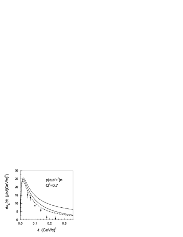
Figure 5: Longitudinal cross section $d\sigma_{L}/dt$ for the $p(e,e^{\prime}\pi^{+})n$ process calculated using Eqs. (7) and (11) with two different values of $\Lambda_{\pi}=$ 0.6 GeV/$c$ (dashed lines) and 1.2 GeV/$c$ (dash-dotted lines). Solid lines: predictions of the scalar ${}^{3}P_{0}$ model ($b_{\pi}=$ 0.3, $b=$ 0.6 fm). Experimental data for $Q^{2}=$ 0.7 (W=2.19 GeV) from Ref. [12] (a) and for 3.3 $GeV^{2}/c^{2}$ (W=2.65 GeV) from Ref. [13] (b).

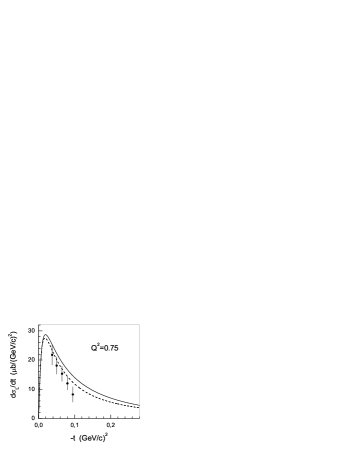
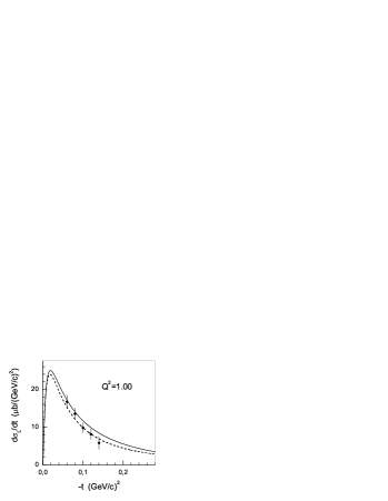
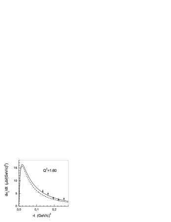
Figure 6: Longitudinal cross section $d\sigma_{L}/dt$ for the $p(e,e^{\prime}\pi^{+})n$ process. The same notations as in Fig. 5. Experimental data from Ref. [14]. $Q^{2}=$ 0.6 (a), 0.75 (b), 1.0 (c), and 1.6 (d) $GeV^{2}/c^{2}$, W=1.95 GeV.

Various phenomenological versions of momentum distribution (MD) of pions in the channel $N\to N+\pi$ are presented in Fig. 4. The solid line corresponds to the MD calculated using Eqs. (11), (12) with the experimental value $g_{\pi{\scriptscriptstyle NN}}=$ 13.2. The cut-off parameter $\Lambda_{\pi}=$ 0.6 GeV/$c$ taken in the calculations reasonably fits the experimental data (see Figs. 5 and 6, dashed lines) in the area $Q^{2}\gtrsim$ 1 $(GeV/c)^{2}$ of $t$-pole bright predominance.

The dashed line in Fig. 4 is MD calculated by means of Eq. (15) using Afnan’s $\pi N$ potential [15], and the dash-dotted line corresponds to MD calculated by means of Eq. (15) using Lee’s $\pi N$ potential [16]. We see that the latter is rather far from the solid line and, consequently, from the experimental data. The calculations based on the Afnan’s potential fit the experimental data rather well.

One can clearly see from Figs. 5 and 6 that our $t$-pole microscopic approach works well at $Q^{2}\gtrsim$ 1 $(GeV/c)^{2}$: both the absolute value of cross section $d\sigma_{\scriptscriptstyle L}/dt$ and the shape of its dependence on $t=-{\bf k}^{2}$ (i.e. the shape of $|\Psi_{p}^{n\pi^{+}}({\bf k}^{2})|^{2}$) are well reproduced by the microscopic theory normalized to the low-energy pion-nucleon data (solid line). At the same time at $Q^{2}\lesssim$ 1 $(GeV/c)^{2}$ the pole approximation is not efficient, what is in a good agreement with our previous estimations [5] (the disturbing influence of the competing $s$-pole diagram and of the $t$-pole diagram with a virtual $\rho$-meson becomes to be essential here [5]).

Further, our discussed results show (see Fig. 7a) that both the shape of phenomenological monopole form factor (12) and the empirical value 0.6$\div$0.7 GeV/c of the cut-off parameter $\Lambda_{\pi}$ (it appears close to that by Phandaripande et al. [34] connected to a phenomenological analysis of independent problems) find its microscopic foundation. In particular, it means that the rms radius of the nucleon is reproduced correctly by these soft cut-off parameters.

So, our predictions for $N\to B+\pi$ channels ($B=\Delta,N_{1/2^{-}}(1535),N_{1/2^{+}}(1440)$) seem to be useful estimates for future exclusive experiments.

4.2 $N\to B+\pi$ channels in the microscopic model

Form factors (56) calculated within the quark ${}^{3}P_{0}$ model for all considered channels $N\to B+\pi$ are presented in Fig. 7(a). For comparison, we also show here for the $N\to N+\pi$ channel the monopole form factor (12) for $\Lambda_{\pi}=$ 0.6 and 0.7 GeV/$c$ (dotted lines), which was discussed above. The $N\to\Delta+\pi$ channel is characterized by the same form factor as the $N\to N+\pi$ channel. However, the MD will be different, first, because of the difference in the pole denominators in Eq. (4) (for $B=\Delta$, $N^{*}$, $N^{**}$ these denominators are bigger than for $B=N$ and are almost ${\bf k}^{2}$-independent). Second, the vertex constants for the $p\to\pi+n$ and $p\to\pi+\Delta$ channels are also different. For comparison the pion momentum distributions for these channels are shown in Fig. 8.

Of particular interest is the dependence of $NB\pi$ vertex functions on the pion radius $b_{\pi}$. The general feature is that all form factors for transitions without radial or orbital excitation of the quark wave function (e.g., $N\to N$, $N\to\Delta$, $N\to\Lambda$) are practically independent from the parameter $x_{\pi}=b_{\pi}/b$ ($x_{\scriptscriptstyle K}=b_{\scriptscriptstyle K}/b$). However, the vertex constants depend strongly on $x_{\pi}$. The ratio $R=g_{\pi BN}^{2}/g_{\pi NN}^{2}$ calculated within the microscopical model considered for the channels $B=N^{*}$, $N^{**}$ is presented in Fig. 7(b) as a function of $x_{\pi}$. The measurements of the $p(e,e^{\prime}\pi)B$ cross-sections will provide us, in particular, with the relative values $g_{\pi BN}^{2}/g_{\pi NN}^{2}$. The comparison of the predicted ratios to the experiment should be essential in the verification of this model including independent obtaining of the $x_{\pi}$ value and its comparison with that which follows from the shape of the pion electromagnetic form factor [in this work we use only the last experimental data [14] on the pion off-shell charge form factor $F_{\pi}(Q^{2})$].

For the channel $B=\Delta$ the ratio $R$ does not depend on $x_{\pi}$, $R=(3\sqrt{2}(M_{\scriptscriptstyle\Delta}+M_{\scriptscriptstyle N})/5M_{\scriptscriptstyle N})^{2}=$ 3.85. We have obtained the following values of $NB\pi$ coupling constants for the point-like pion ($x_{\pi}=0$): $g_{\pi\Delta N}^{2}/4\pi=53.4$, $g_{\pi N^{*}N}^{2}/4\pi=11.8$ and $g_{\pi N^{**}N}^{2}/4\pi=$ 2.1, while at $x_{\pi}=0.5$ the $\pi NN^{**}$ coupling constant becomes larger: $g_{\pi N^{**}N}^{2}/4\pi=$ 3.09 (see Fig. 7(b)).

The form factors for transitions with orbital or radial excitation (i.e. for the $B=N^{*}$ and $N^{**}$ channels) depend on the $x_{\pi}$. Assuming $x_{\pi}=$ 0.5 we have obtained that these form factors change the sign at $|{\bf k}^{2}|\simeq$ 1.22 and 0.72 (GeV/$c$)². It could be considered as a manifestation of the excited quark configurations $s^{2}p$ and $sp^{2}$ in baryons $N^{*}$ and $N^{**}$ respectively. This is a directly observable effect.

4.3 $N\to Y+K$ channels

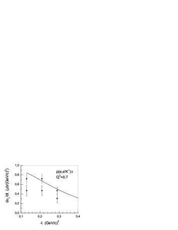
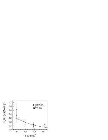
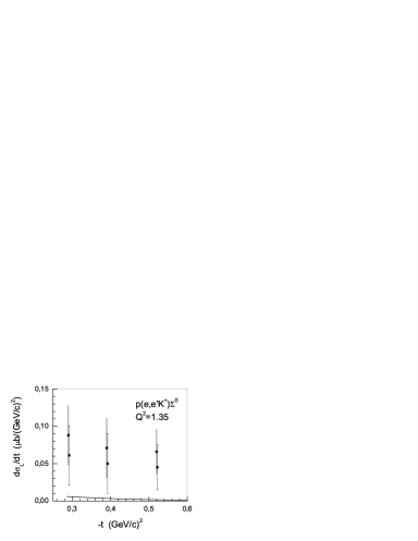
Figure 10: Kaon quasi-elastic knockout cross sections $p(e,e^{\prime}K^{+})\Lambda$ (a,b) and $p(e,e^{\prime}K^{+})\Sigma^{0}$ (c,d). Solid lines: the scalar ${}^{3}P_{0}$ model ($b_{\pi}=$ 0.3 fm, $b=$ 0.6 fm, $z=$ 0.5). Data from P.Brauel et al. [12] (modified): circles for $R\equiv\sigma_{L}/\sigma_{T}=$ 1. and squares for $R=$ 0.5; $Q^{2}=$ 0.7 $GeV^{2}/c^{2}$ (a,c), $Q^{2}=$ 1.35 $GeV^{2}/c^{2}$ (b,d); $W=$ 1.9$\div$2.5 GeV.

Our calculations of the MDs of kaons in the channels $p\to\Lambda+K$ and $p\to\Sigma+K$ within the ${}^{3}P_{0}$ model are shown in Fig. 9. Predicted spectroscopic factors are $S^{K\Lambda}_{p}=0.152$ and $S^{K\Sigma}_{p}=0.006$ (for comparison $S^{\pi N}_{N}=0.25$). The corresponding cross sections are presented in Fig. 10.

Unfortunately, the longitudinal $d\sigma_{\scriptscriptstyle L}/dt$ and transverse $d\sigma_{\scriptscriptstyle T}/dt$ differential cross sections of the channel $N\to Y+K$ are not separated in the available data, and we cannot extract the MD of kaons from the experiment as we did it for pions. Ref. [13] gives us only the ratio of these cross sections $R=(d\sigma_{\scriptscriptstyle L}/dt)/(d\sigma_{\scriptscriptstyle T}/dt)\approx$ 1 in the narrow range $t=0.33-0.38$ $GeV^{2}/c^{2}$ for $\Lambda+K^{+}$ channel and $t=0.25-0.3$ $GeV^{2}/c^{2}$ for $\Sigma^{0}+K^{+}$ channel. Recently [38] the ratio $R^{\prime}=(d\sigma_{\scriptscriptstyle L}/d\Omega)/(d\sigma_{\scriptscriptstyle T}/d\Omega)\approx$ 0.5 was measured in the $p(e,e^{\prime}K^{+})\Lambda$ reaction for zero angle $\theta_{\scriptscriptstyle K}$ of kaon emission with respect to the photon momentum ${\bf q}^{cm}$ in the area 0.5 $<Q^{2}<$ 2. $(GeV/c)^{2}$.

Having in mind the large spread of experimental data, we consider here two variants, $R=$ 0.5 and $R=$ 1. Using the old DESY data [12] on $d\sigma/dt=\varepsilon d\sigma_{L}/dt+d\sigma_{T}/dt$ for $Q^{2}=$ 0.7 and 1.35 $(GeV/c)^{2}$ at $\varepsilon=$ 0.85 and 0.82 (W = 1.9 $\div$ 2.5 GeV) for both $p\to\Lambda+K^{+}$ and $p\to\Sigma^{0}+K^{+}$ channels we have estimated the longitudinal cross section as $d\sigma_{L}/dt=\frac{R}{R+\varepsilon}\,d\sigma/dt$. With these data for $\Lambda+K^{+}$ channel (see Fig. 10(a,b)) we have estimated the value of the parameter $z$ in Eq. (68), $z\approx$ 0.4$\div$0.5. In Figs. 10(a-d) and 11(a,b) the predictions of the scalar ${}^{3}P_{0}$ model for longitudinal cross sections of quasi-elastic kaon knockout from the proton are shown (solid line) for both channels $\Lambda+K$ and $\Sigma^{0}+K$ with using the value $z=$ 0.5.

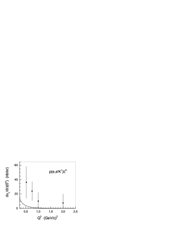
Figure 11: $Q^{2}$-dependence of the longitudinal kaon quasi-elastic knockout differential cross section $d\sigma_{L}/d\Omega$ at zero angle to the photon direction: (a) $p(e,e^{\prime}K^{+})\Lambda$, (b) $p(e,e^{\prime}K^{+})\Sigma^{0}$. Solid lines: the scalar ${}^{3}P_{0}$ model ($b_{\pi}=$ 0.3, $b=$ 0.6 fm, $z=$ 0.5). Data from Ref. [38].

The $Q^{2}$-dependence of the differential cross sections $d\sigma_{L}/d\Omega$ for $\theta_{\scriptscriptstyle K}=0^{o}$ is shown on Fig.11 (solid line). For this dependence there exists separated experimental data for the longitudinal and transverse differential cross sections [38], but this dependence does not give us the shape of the MDs. For example, at $Q^{2}\gtrsim$ 1 $(GeV/c)^{2}$ these zero-angle data correspond to too large virtual-pion momenta ${\bf k}^{2}\gtrsim$ 0.5 $(GeV/c)^{2}$ to be described in terms of merely kaon t-pole diagrams.

Note, that the theoretical calculations within the ${}^{3}P_{0}$ model do not reproduce the ratio of the longitudinal cross sections for the $N\to\Lambda+K$ and $N\to\Sigma+K$ channels. The theoretical result is $d\sigma_{L}/dt(N\to\Lambda+K):d\sigma_{L}/dt(N\to\Sigma+K)\approx$ $g_{K\Lambda N}^{2}/g_{K\Sigma N}^{2}=27$ (in fact, the ratio of the cross sections is more than 27 due to the difference in mass between $\Lambda$ and $\Sigma$ baryons; it is about 40). The experimental ratio is much smaller. This may be an indication of the fact that another mechanism contributes considerably to the cross section. For example, an enhancement of the $K\Sigma^{0}$ amplitude as it was pointed out in Ref. [38] may originate from s-channel $\Delta^{*}$ resonances which are forbidden by isospin in the $K\Lambda$ system.

Recall that the ratio $g_{K\Lambda N}^{2}/g_{K\Sigma N}^{2}=27$ within the scalar ${}^{3}P_{0}$ model is a consequence of Eqs. (63) and (64), which, in turn, is a result of $SU(6)$ spin-flavor symmetry of initial interaction Hamiltonian (20). To obtain absolute values of these constants we must normalize the only free parameter of the model, $g_{s}$, to a known vertex constant $g_{\pi NN}$, and it gives $g_{\scriptscriptstyle K\Lambda N}/\sqrt{4\pi}=$ -5.1 , $g_{\scriptscriptstyle K\Sigma N}/\sqrt{4\pi}=$ 1.0, if $z=$ 1, but in a more realistic case, when $z=$ 0.5, it gives $g_{\scriptscriptstyle K\Lambda N}/\sqrt{4\pi}=-2.53$ , $g_{\scriptscriptstyle K\Sigma N}/\sqrt{4\pi}=0.51$. For comparison, Refs. [35, 36] give us the following values: $g_{\scriptscriptstyle K\Lambda N}/\sqrt{4\pi}=-3.16$, $g_{\scriptscriptstyle K\Sigma N}/\sqrt{4\pi}=0.91$ [35] and $g_{\scriptscriptstyle K\Lambda N}/\sqrt{4\pi}=-4.17$, $g_{\scriptscriptstyle K\Sigma N}/\sqrt{4\pi}=1.18$ [36].

To refine these values and to clarify the origin of enhancement of the $p\to\Sigma+K$ cross section the measurement of kaonic MDs in the channels $p\to\Lambda+K$ and $p\to\Sigma+K$ (both their normalizations and shapes) should be very important.

4.4 Some perspectives

Basing on the microscopical ${}^{3}P_{0}$ model we have predicted the pionic MDs, both the shape of $k$-dependence and normalization, i.e. spectroscopic factor, in the channels of virtual decay $N\to B+\pi$, $B=N$, $\Delta$, $N^{*}$, $N^{**}$, and kaonic MDs in the channels $N\to Y+K$, $Y=\Lambda$, $\Sigma$. The microscopic consideration can be easily extended to higher excited states of the baryon-spectator $B$ using the more advanced relativistic version of the ${}^{3}P_{0}$ model. These MDs can be efficiently verified in the quasi-elastic knockout experiments $p(e,e^{\prime}\pi)B$ and $p(e,e^{\prime}K)Y$ at the electron beam energy of a few GeV. Such broad verification should be an important ground for further improvement of microscopical quark models, which provide us with the valuable universal basis for consideration of various meson clouds. Our nearest intention here consists in consideration of the transverse cross section $d\sigma_{T}/dt$ of the process $p(e,e^{\prime}\pi)B$. It opens a way to the investigation of the $\rho$-meson MD $\overline{|\Psi_{p}^{n\rho}({\bf k})|^{2}}$ via very predominating (at $Q^{2}=2-4$ GeV²/$c^{2}$) virtual subprocess $\rho^{*}+\gamma_{T}^{*}\to\pi$ ($*$ means a virtual particle). Analogously, we plan to calculate microscopically the MDs of vector strange mesons which can be extracted from the transverse cross sections $d\sigma_{\scriptscriptstyle T}/dt$ of $p(e,e^{\prime})Y$ quasi-elastic knockout processes.

Further, as a next step, an amplitude of a non-diagonal subprocess $\pi^{*}(L)+\gamma^{*}\to\pi(L=0)$ with rearrangement of the nonzero internal orbital momentum $L$ of the virtual pion $\pi^{*}$ to $L=0$ can be extracted from the properly organized experiment, if we take into account our experience in the physics of clusters in the nucleus. Namely, the theory of quasi-elastic knockout of clusters from nuclei by intermediate energy protons [4, 22] shows that the amplitudes of deexcitation of virtually excited clusters [say, $\alpha^{*}(L\neq 0)+p\to\alpha(L=0)+p^{\prime}$] play very important role here. These amplitudes can be revealed by very large anisotropies of differential cross sections in regards to the orientation of the recoil momentum ${\bf k}$ of the final nucleus-spectator $A-4$ with respect to the bombarding beam direction ($\theta$-anisotropy) and to proton scattering plane ($\phi$-anisotropy, i.e. Treiman-Yang anisotropy [4, 22]). For electrons with only single electron-quark collisions, the effect will be probably not so big, but quite observable [39].

It seems reasonable to join the above microscopic approach with virtually excited mesons in the nucleon and the experience of the phenomenological theory of Regge poles as applied to the analysis of electroproduction of pions and kaons [40]. Such synthesis can illuminate microscopical ground of the Regge theory.

The present paper, where we use a ”naive” non-relativistic model of scalar ${}^{3}P_{0}$ fluctuation, aims to outline preliminarily a new horizon in both experimental and theoretical intermediate energy research of nonpertubative QCD as a basis for detailed explanations and predictions of various meson-baryon degrees of freedom.

Acknowledgments

We gratefully acknowledge very useful discussions with Prof. A. Faessler and Dr. V. Lyubovitskij. This work was partially supported by the Russian Foundation for Basic Research (grant N 03-02-17394) and the Deutsche Forshungsgemainschaft (grant Fa67/20-1).

Figure captions

Fig.1. Feynman $t$-pole diagram for the pion production off the nucleon: a) the quasi-elastic knockout of pion; b) $z$-diagram of $\pi^{+}\pi^{-}$ production.

Fig.2. Quark microscopic picture of pion production inside the nucleon.

Fig.3. The effective quark-pion vertex of the scalar ${}^{3}P_{0}$ model.

Fig.4. Momentum distribution of pions in the nucleon. The “radial” part $|R_{p}^{n\pi^{+}}({\bf k}^{2})|^{2}$, $(GeV/c)^{-3}$, versus ${\bf k}^{2}$: the solid line for the wave function (11); the dashed line for the function (15) calculated on the basis of Ref. [15] model; the dash-dotted line for the function (15) calculated on the basis of Ref. [16] model.

Fig.5. Longitudinal cross section $d\sigma_{L}/dt$ for the $p(e,e^{\prime}\pi^{+})n$ process calculated using Eqs. (7) and (11) with two different values of $\Lambda_{\pi}=$ 0.6 GeV/$c$ (dashed lines) and 1.2 GeV/$c$ (dash-dotted lines). Solid lines: predictions of the scalar ${}^{3}P_{0}$ model ($b_{\pi}=$ 0.3, $b=$ 0.6 fm). Experimental data for $Q^{2}=$ 0.7 (W=2.19 GeV) from Ref. [12] (a) and for 3.3 $GeV^{2}/c^{2}$ (W=2.65 GeV) from Ref. [13] (b).

Fig.6. Longitudinal cross section $d\sigma_{L}/dt$ for the $p(e,e^{\prime}\pi^{+})n$ process. The same notations as in Fig. 5. Experimental data from Ref. [14]. $Q^{2}=$ 0.6 (a), 0.75 (b), 1.0 (c), and 1.6 (d) $GeV^{2}/c^{2}$, W=1.95 GeV.

Fig.7. (a) Strong form factors in the scalar ${}^{3}P_{0}$ model ($b_{\pi}=$ 0.3 fm, $b=$ 0.6 fm): $F_{\pi NN}$ (solid line), $F_{\pi NN^{**}}$ (dashed line), $F_{\pi NN^{*}}$ (dash-dotted line). Dotted lines correspond to the form factor parametrized by Eq. (12) with $\Lambda_{\pi}=$ 0.7 $GeV^{2}/c^{2}$ (upper line) and 0.6 $GeV^{2}/c^{2}$ (lower line). (b) The scalar ${}^{3}P_{0}$ model. The ratio of strong coupling constants R $=g^{2}_{\pi NB}/g^{2}_{\pi NN}$ for $B=N^{**}\equiv N_{1/2^{+}}(1440)$ (solid line) and for $B=N^{*}\equiv N_{1/2^{-}}(1535)$ (dashed line); $x=b_{\pi}/b$

Fig.8. Momentum distribution of pions in the proton; solid line: $p\to\pi+n$ channel, dashed line: $p\to\pi+\Delta$ channel. The scalar ${}^{3}P_{0}$ model.

Fig.9. Momentum distribution of kaons in the proton; solid line: the $p\to K+\Lambda$ channel, dashed line: the $p\to K+\Sigma$ channel (times 10). The scalar ${}^{3}P_{0}$ model.

Fig.10. Kaon quasi-elastic knockout cross sections $p(e,e^{\prime}K^{+})\Lambda$ (a,b) and $p(e,e^{\prime}K^{+})\Sigma^{0}$ (c,d). Solid lines: the scalar ${}^{3}P_{0}$ model ($b_{\pi}=$ 0.3 fm, $b=$ 0.6 fm, $z=$ 0.5). Data from P.Brauel et al. [12] (modified): circles for $R\equiv\sigma_{L}/\sigma_{T}=$ 1. and squares for $R=$ 0.5; $Q^{2}=$ 0.7 $GeV^{2}/c^{2}$ (a,c), $Q^{2}=$ 1.35 $GeV^{2}/c^{2}$ (b,d); $W=$ 1.9$\div$2.5 GeV.

Fig.11. $Q^{2}$-dependence of the longitudinal kaon quasi-elastic knockout differential cross section $d\sigma_{L}/d\Omega$ at zero angle to the photon direction: (a) $p(e,e^{\prime}K^{+})\Lambda$, (b) $p(e,e^{\prime}K^{+})\Sigma^{0}$. Solid lines: the scalar ${}^{3}P_{0}$ model ($b_{\pi}=$ 0.3, $b=$ 0.6 fm, $z=$ 0.5). Data from Ref. [38].

Figure 2: Quark microscopic picture of pion production inside the nucleon.

Figure 3: The effective quark-pion vertex of the scalar ${}^{3}P_{0}$ model.

Figure 4: Momentum distribution of pions in the nucleon. The “radial” part $|R_{p}^{n\pi^{+}}({\bf k}^{2})|^{2}$, $(GeV/c)^{-3}$, versus ${\bf k}^{2}$: the solid line for the wave function (11); the dashed line for the function (15) calculated on the basis of Ref. [15] model; the dash-dotted line for the function (15) calculated on the basis of Ref. [16] model.

 

   

 

Figure 7: (a) Strong form factors in the scalar ${}^{3}P_{0}$ model ($b_{\pi}=$ 0.3 fm, $b=$ 0.6 fm): $F_{\pi NN}$ (solid line), $F_{\pi NN^{**}}$ (dashed line), $F_{\pi NN^{*}}$ (dash-dotted line). Dotted lines correspond to the form factor parametrized by Eq. (12) with $\Lambda_{\pi}=$ 0.7 $GeV^{2}/c^{2}$ (upper line) and 0.6 $GeV^{2}/c^{2}$ (lower line). (b) The scalar ${}^{3}P_{0}$ model. The ratio of strong coupling constants R $=g^{2}_{\pi NB}/g^{2}_{\pi NN}$ for $B=N^{**}\equiv N_{1/2^{+}}(1440)$ (solid line) and for $B=N^{*}\equiv N_{1/2^{-}}(1535)$ (dashed line); $x=b_{\pi}/b$.

Figure 8: Momentum distribution of pions in the proton; solid line: $p\to\pi+n$ channel, dashed line: $p\to\pi+\Delta$ channel. The scalar ${}^{3}P_{0}$ model.

Figure 9: Momentum distribution of kaons in the proton; solid line: the $p\to K+\Lambda$ channel, dashed line: the $p\to K+\Sigma$ channel (times 10). The scalar ${}^{3}P_{0}$ model.

References

• [1] E. Weigold and I. McCarthy, Electron Momentum Spectroscopy. Kluver Academic Plenum Publishers, N.Y., 1999.
• [2] V.G. Neudatchin, Yu.V. Popov, and Yu.F. Smirnov, Uspekhi Fiz. Nauk, 69, 1111 (1999).
• [3] S.S. Volkov, A.A. Vorobiev, O.A. Domchenkov, et al., Yad.Fiz. 52, 1339 (1990); A.A. Vorobiev, Yu.V. Dotsenko, A.A. Lobodenko et al., Yad.Fiz. 58, 3 (1994); D.G. Ireland, and G. Van Der Steenhoven, Phys.Rev. C 49, 2182 (1994); J.Ryckebush, W. Van Nespen, and S. Janssen, Phys.Rev. C 62, 024611 (2000).
• [4] V.G. Neudatchin, A.A. Sakharuk, V.V. Kurovsky, and Yu.M. Tchuvilsky, Phys.Rev. C 50, 148 (1994); Phys.Rev. C 51, 784 (1995).
• [5] V.G. Neudatchin, L.L. Sviridova, and N.P. Yudin, Yad. Fiz. 64, 1680 (2001).
• [6] V.G. Neudatchin, L.L. Sviridova, and N.P. Yudin, Yad. Fiz. 65, 1598 (2002).
• [7] V.V. Balashov and A.N. Boyarkina, Nucl.Phys. 38, 629 (1962); K. Dietrich, Phys.Lett. 2, 139 (1962).
• [8] J. Güttner, G. Chanfray, H.J. Pirner, and B. Povh, Nucl. Phys. A 429, 389 (1984); J.D. Sullivan, Phys.Rev. D 5, 1732 (1972).
• [9] J. Speth, V.R. Zoller, Phys.Lett. B 351, 533 (1995).
• [10] N.P. Yudin, L.L. Sviridova, and V.G. Neudatchin, Yad. Fiz. 65, 594 (2002).
• [11] Yu.V. Novozhilov. Introduction to the theory of elementary particles. Moscow, Nauka, 1972 (in Russian).
• [12] P. Brauel, T. Canzler, D. Cords, et al., Z.Phys. C 3, 101 (1979);
• [13] C.J. Bebek, C.N. Brown, S.D. Holmes, et al., Phys.Rev. D 17, 1693 (1978) ).
• [14] J. Volmer, D. Abbott, H. Anklin, et el., Phys.Rev.Lett. 86, 1713 (2001).
• [15] T.-Y. Saito, I.R. Afnan, Few-Body Systems 18, 101 (1995).
• [16] S. Nozawa, B. Blankleider, and T.-S. H. Lee, Nucl.Phys. A 513, 459 (1990).
• [17] N. Isgur, Phys. Rev. D 32, 189 (1985); S. Godfrey and N. Isgur, Phys. Rev. D 34, 2809 (1986); R. Kokoski and N. Isgur, Phys. Rev. D 35, 907 (1987); S. Kapstick and W. Roberts, Phys. Rev. D 49, 4570 (1994); P. Geiger and E.S. Swanson, Phys. Rev. D 50, 6855 (1994).
• [18] P. Stassart and Fl. Stancu, Phys. Rev. D 42, 1521 (1990); P. Stassart, Phys. Rev. D 42, 1521 (1990).
• [19] A. Le Yaouanc, L. Oliver, O. Péne, and J. Raynal, Phys. Lett. 71B, 397 (1977): 72B, 57 (1977): P. R. Page, Nucl. Phys. B446, 189 (1995).
• [20] B. Desplanques, C. Gignoux, B. Silvestre-Brac et al., Z.Phys. A 343, 331 (1992); F. Cano, P. Gonzalez, S. Noguera, B. Desplanques, Nucl.Phys. A 603, 257 (1996); P.J.A. Bicudo, L.S. Ferreira, C.M. Placido, J. Ribeiro, Phys.Rev. C 56, 670 (1997).
• [21] E.S. Ackleh, T.D. Barns and E.S. Swanson, Phys. Rev. D 54, 6811 (1996).
• [22] N.F. Golovanova, I.M. Il’in, V.G. Neudatchin et al., Nucl. Phys. A 262, 444 (1976); Nucl.Phys. A 285, 531 (1977); V.G. Neudatchin, Yu.F. Smirnov and N.F. Golovanova, Adv. in Nucl. Phys. 11, 1-133 (1979).
• [23] M. Strikman, Nucl. Phys. A 663-664, 64c (2000); M. Vanderhaeghen, P.A. Guichon, and M. Guidal, Nucl. Phys. A 663-664, 324c (2000).
• [24] V. Dmitrasinovich, F. Gross, Phys.Rev. C 40, 2479 (1989); P.J. Mulders, Phys.Rep. 185, 83 (1990); S. Boffi, C. Giusi, F.D. Pacati, Phys.Rep. 226, 1 (1993).
• [25] L.D. Blokhintsev, I. Borbeli, and E.I. Dolinsky, Sov. J. Part. Nucl. 8, 485 (1977); R.N. Faustov, V.O. Galkin, A.I. Mishurov, Phys. Lett. B 356, 516 (1995).
• [26] J. Gronberg et al., Phys. Rev. D 57, 33 (1998).
• [27] S. Godfrey and N. Isgur, Phys. Rev. D 32, 189 (1985).
• [28] J. Volmer, D. Abbott, H. Anklin et al., Phys. Rev. Lett. 86, 1713 (2001).
• [29] C. Itzykson and J.-B. Zuber, Quantum Field Theory. McGraw-Hill Book Company, N.Y. 1980.
• [30] D.O. Riska and G.E. Brown, Nucl.Phys. A 679, 577 (2001).
• [31] I.T. Obukhovsky, A.Faessler, G. Wagner, and A. Buchmann, Phys. Rev. C 60, 035207 (1999).
• [32] L.Ya. Glozman, V.G. Neudatchin, and I.T. Obukhovsky, Phys.Rev. C 48, 389 (1993); L.Ya. Glozman and A. Faessler, Phys. Lett. B 348, 270 (1995).
• [33] B.T. Feld, Models of Elementary Particles. Blaisdell Publishing Company, London. 1969.
• [34] S. Loucks, V.R. Phandaripande, and R. Schiavilla, Phys. Rev. C 49, 342 (1994); Phys. Rev. 149, 1 (1987).
• [35] J.C. David, G. Fayard, G.H. Lamot, B. Saghai, Phys.Rev. C 53, 2613 (1996).
• [36] R.A. Adelseck, B. Saghai, Phys.Rev. C 42, 108 (1990); R.A. Adelseck et al., Phys.Rev. C 45, 2030 (1992).
• [37] L. Theussl, R.F. Wagenbrunn, B. Desplanques, and W. Plessas, nucl-th/0010099; F. Cano, B. Desplanque, P. Gonzalez, and S. Noquera, nucl-th/0102013.
• [38] R.M. Mohring, D. Abbott, A. Ahmidouch, et al., Phys.Rev. C 67, 055205 (2003).
• [39] A.A. Sakharuk, V.G. Zelevinsky, and V.G. Neudatchin, Phys.Rev. C 60, 014605 (1999).
• [40] M. Guidal, J.-M. Laget, M. Vanderhaeghen, Nucl.Phys. A 627, 645 (1997).