1 Introduction

Can the radiation pattern of an antenna be isotropic?

A simple argument suggests that this is difficult.

The intensity of radiation depends on the square of the electric (or magnetic) field. To have isotropic radiation, it would seem that the magnitude of the electric field would have to be uniform over any sphere in the far zone. However, the electromagnetic fields in the far zone of an antenna are transverse, and it is well known that a vector field of constant magnitude cannot be everywhere tangent to the surface of a sphere (Brouwer’s “hairy-ball theorem” [1]). Hence, it would appear that the transverse electric field in the far zone cannot have the same magnitude in all directions, and that the radiation pattern cannot be isotropic, IF the radiation is everywhere linearly polarized [2, 3].

However, electromagnetic waves can have two independent states of polarization, described as elliptical polarization in the general case. While a transverse electric field with a single, linearly polarized component cannot be uniform over a sphere in the far zone, it may be possible that the sum of the squares of the electric fields with two polarizations is uniform.

2 The U-Shaped Antenna of Shtrikman

Shmuel Shtrikman has given an example of a U-shaped antenna that generates an isotropic radiation pattern in the far zone [4] in the limit of zero intensity of the radiation. This example shows that any desired degree of “isotropicity” can be achieved for a sufficiently weak radiation pattern.

Matzner [5] has also shown that the radiation pattern of the U-shaped antenna can in principle be produced by specified currents of finite strength on the surface of a sphere.

2.1 The U-Shaped Antenna

The U-shaped antenna of Matzner et al. [4] is illustrated in Fig. 1. It consists of two vertical arms of length $L=\lambda/4$ $(kL=\pi/2)$, separated by a short cross piece of length $h\ll\lambda$.

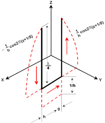
Figure 1: The U-shaped antenna whose radiation pattern is isotropic in the limit that $h\to 0$, for which the intensity also goes to zero. The dashed lines indicate the spatial dependence of the current. From [4].

Denoting the peak current in the antenna by $I$, the current density J can be written

$${\bf J}({\bf r},t)={\bf J}({\bf r})e^{-i\omega t},$$ (1)

where

$${\bf J}({\bf r}) = I\left[\delta(x-h/2)\delta(y)\cos(kz+\pi/4)\hat{\bf z}\right.+\ \delta(y)\delta(z+\lambda/8)\hat{\bf x}$$ (2)

$$\left.-\ \delta(x+h/2)\delta(y)\cos(kz+\pi/4)\hat{\bf z}\right],$$

and $-\lambda/8\leq z\leq\lambda/8$ on the vertical arms, $-h/2\leq x\leq h/2$ on the horizontal arm.

The time-averaged, far-zone radiation pattern of an antenna with a specified, time-harmonic current density can be calculated (in Gaussian units) according to [6]

$${dP\over d\Omega}={\omega^{2}\over 8\pi c^{3}}\left|\hat{\bf k}\times\left[\hat{\bf k}\times\int{\bf J}({\bf r})e^{i{\bf k}\cdot{\bf r}}d{\rm Vol}\right]\right|^{2}.$$ (3)

For an observer at angles $(\theta,\phi)$ with respect to the $z$ axis (in a spherical coordinate system), the unit wave vector has rectangular components

$$\hat{\bf k}=\sin\theta\cos\phi\ \hat{\bf x}+\sin\theta\sin\phi\ \hat{\bf y}+\cos\theta\ \hat{\bf z}.$$ (4)

The integral transform ${\bf J}_{k}=\int{\bf J}({\bf r})e^{i{\bf k}\cdot{\bf r}}d{\rm Vol}$ in eq. (3) has rectangular components

$$J_{k,x} = I\int_{-h/2}^{h/2}dxe^{ik\sin\theta\cos\phi x}\int dy\delta(y)e^{ik\sin\theta\sin\phi y}\int dz\delta(z+1/8)e^{ik\cos\theta z}$$ (5)

$$= I{\sin[(k/2)h\sin\theta\cos\phi]\over(k/2)\sin\theta\cos\phi}e^{-i(\pi/4)\cos\theta}\approx Ihe^{-i(\pi/4)\cos\theta},$$

$$J_{k,y} = 0,$$ (6)

$$J_{k,z} = I\int dx\delta(x-h/2)e^{ik\sin\theta\cos\phi x}\int dy\delta(y)e^{ik\sin\theta\sin\phi y}\int_{-\lambda/8}^{\lambda/8}dz\cos(kz+\pi/4)e^{ik\cos\theta z}$$ (7)

$$-I\int dx\delta(x+h/2)e^{ik\sin\theta\cos\phi x}\int dy\delta(y)e^{ik\sin\theta\sin\phi y}\int_{-\lambda/8}^{\lambda/8}dz\cos(kz+\pi/4)e^{ik\cos\theta z}$$

$$= I{\sin[(k/2)h\sin\theta\cos\phi]\over(k/2)\sin^{2}\theta}(ie^{i(\pi/4)\cos\theta}+\cos\theta e^{-i(\pi/4)\cos\theta})$$

$$\approx Ih{\cos\phi\over\sin\theta}(ie^{i(\pi/4)\cos\theta}+\cos\theta e^{-i(\pi/4)\cos\theta}).$$

Then,

$$\left|\hat{\bf k}\times\left(\hat{\bf k}\times{\bf J}_{k}\right)\right|^{2} = |{\bf J}_{k}|^{2}-|\hat{\bf k}\cdot{\bf J}_{k}|^{2}$$ (8)

$$= (1-\hat{k}_{x}^{2})|J_{k,x}|^{2}+(1-\hat{k}_{z}^{2})|J_{k,z}|^{2}-2\hat{k}_{x}\hat{k}_{z}ReJ_{k,x}J^{\star}_{k,z}$$

$$= (1-\sin^{2}\theta\cos^{2}\phi)|J_{k,x}|^{2}+\sin^{2}\theta|J_{k,z}|^{2}-2\sin\theta\cos\theta\cos\phi ReJ_{k,x}J^{\star}_{k,z}$$

$$= I^{2}{\sin^{2}[(k/2)h\sin\theta\cos\phi]\over[(k/2)\pi\sin\theta\cos\phi]^{2}}\left[(1-\sin^{2}\theta\cos^{2}\phi)\right.$$

$$\qquad+\cos^{2}\phi(1+\cos^{2}\theta-2\cos\theta\sin[(\pi/2)\cos\theta])$$

$$\qquad\left.-2\cos^{2}\phi(\cos^{2}\theta-\cos\theta\sin[(\pi/2)\cos\theta])\right]$$

$$= I^{2}{\sin^{2}[(k/2)h\sin\theta\cos\phi]\over[(k/2)\sin\theta\cos\phi]^{2}}\approx I^{2}h^{2}.$$

Thus, the radiation pattern is indeed isotropic in the limit that $h\to 0$. But in this limit, the radiation vanishes, for a fixed peak current $I$.

For a finite separation $h$ between the two vertical arms of the antenna, the deviation from isotropicity is roughly $1-\sin^{2}(kh/2)/(kh/2)^{2}$. Thus the pattern will be isotropic to 1% for $h\sim 0.05\lambda$. However, this uniformity is achieved at the expense of a substantial reduction in the intensity of the radiation. For example, the case of a U-shaped antenna with $h=0.05\lambda$ has an intensity only 1/40 of that of a basic half-wave, center-fed antenna.

As is to be expected, the polarization of the radiation of the U-shaped antenna is elliptical in general. The far-zone electromagnetic fields are related to the integral transform ${\bf J}_{k}$ according to

$${\bf B}=ik{e^{i(kr-\omega t)}\over r}\hat{\bf k}\times{\bf J}_{k},\qquad{\bf E}={\bf B}\times\hat{\bf k}.$$ (10)

The components of the far-zone electromagnetic fields in spherical coordinates are therefore,

$$E_{r}=B_{r} = \hat{\bf k}\cdot{\bf B}=0,$$ (11)

$$E_{\theta}=B_{\phi} = ik{e^{i(kr-\omega t)}\over r}(\cos\theta\cos\phi J_{k,x}-\sin\theta J_{k,z})$$ (12)

$$= Ik\cos\phi e^{i(\pi/4)\cos\theta}{\sin[(k/2)h\sin\theta\cos\phi]\over(k/2)\sin\theta\cos\phi}{e^{i(kr-\omega t)}\over r}$$

$$\approx Ihk\cos\phi e^{i(\pi/4)\cos\theta}{e^{i(kr-\omega t)}\over r}\,,$$

$$E_{\phi}=-B_{\theta} = -ik{e^{i(kr-\omega t)}\over r}\sin\phi J_{k,x}$$ (13)

$$= -iIk\sin\phi e^{-i(\pi/4)\cos\theta}{\sin[(k/2)h\sin\theta\cos\phi]\over(k/2)\sin\theta\cos\phi}{e^{i(kr-\omega t)}\over r}$$

$$\approx -iIhk\sin\phi e^{-i(\pi/4)\cos\theta}{e^{i(kr-\omega t)}\over r}\,.$$

The magnitudes of the fields are

$$E=B={Ik\over r}{\sin[(k/2)h\sin\theta\cos\phi]\over(k/2)\sin\theta\cos\phi}\approx{Ihk\over r}\,,$$ (14)

which are isotropic in the limit of small $h$. Figure 2 from [5] illustrates the character of the elliptical polarization of the fields (12)-(13) for various directions in the limit of small $h$.

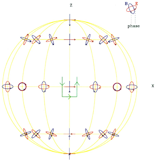
Figure 2: The elliptical polarization of the fields (12)-(13) of the U-shaped antenna in the limit of small $h$. From [5].

2.2 Isotropic Radiation from Currents on a Spherical Shell

In sec. 6.6 of his Ph.D. thesis [5], Matzner shows how the far-zone radiation pattern of the U-shaped antenna (in the limit $h\to 0$) can be reproduced by an appropriate distribution of currents on a spherical shell of radius $R=\lambda/4$. For this, he first expands the far-zone fields (12)-(13) in vector spherical harmonics, and then matches these to currents on a shell of radius $R$ and to an appropriate form for the fields inside the shell.

Figures 3 and 4 illustrate this procedure. The key point is that the surface currents are finite in magnitude, and hence an isotropic radiator is realizable in the laboratory (in contrast to the U-shaped antenna, which requires an infinite current $I$ to achieve perfectly isotropic radiation).

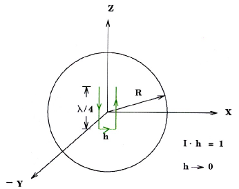
Figure 3: The spherical shell of radius $R=\lambda/4$ on which a set of currents can be found that produces the same far-zone fields as does the U-shaped antenna. From [5].

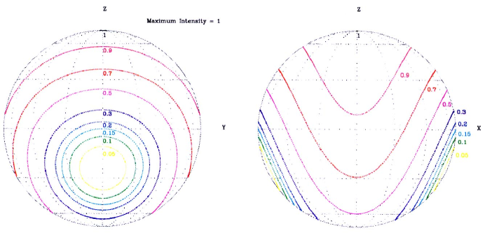
Figure 4: Contours of the current density on the spherical shell that produce the same far-zone fields as does the U-shaped antenna. From [5].

In principle, many other surfaces besides that of a sphere could support a pattern of finite, oscillating currents whose far zone radiation pattern is isotropic.

3 A Linear Array of “Turnstile” Antennas

Saunders [3] has noted that a certain infinite array (a certain vertical stack) of so-called “turnstile” antennas [7, 8] can also produce a far-zone radiation pattern that is isotropic

A turnstile antenna consists of a pair of half-wave, center-fed linear dipole antennas oriented at 90^∘ to each other, and driven 90^∘ out of phase, as shown in Fig. 5.

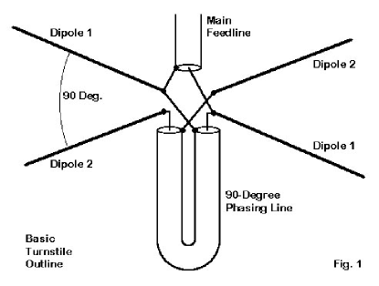
Figure 5: A “turnstile” antenna. From [8].

If we approximate the half-wave dipoles by point dipoles, then the dipole moment of the system can be written

$${\bf p}={\bf p}_{0}e^{-i\omega t}=p_{0}(\hat{\bf x}+i\hat{\bf y})e^{-i\omega t},$$ (15)

taking the antenna to be aligned along the $x$ and $y$ axes. The electromagnetic fields in the far zone are then

$${\bf B}=k^{2}{e^{i(kr-\omega t)}\over r}\hat{\bf k}\times{\bf p}_{0},\qquad{\bf E}={\bf B}\times\hat{\bf k},$$ (16)

whose components in spherical coordinates are

$$E_{r}=B_{r} = \hat{\bf k}\cdot{\bf B}=0,$$ (17)

$$E_{\theta}=B_{\phi} = -p_{0}k^{2}{e^{i(kr-\omega t)}\over r}\cos\theta(\cos\phi+i\sin\phi),$$ (18)

$$E_{\phi}=-B_{\theta} = -p_{0}k^{2}{e^{i(kr-\omega t)}\over r}(\sin\phi-i\cos\phi).$$ (19)

In the plane of the antenna, $\theta=90^{\circ}$, the electric field has no $\theta$ component, and hence no $z$ component; the turnstile radiation in the horizontal plane is horizontally polarized. In the vertical direction, $\theta=0^{\circ}$ or $180^{\circ}$, the radiation is circularly polarized. For intermediate angles $\theta$ the radiation is elliptically polarized.

The magnitudes of the fields are

$$E=B={p_{0}k^{2}\over r}\sqrt{1+\cos^{2}\theta},$$ (20)

so the time-averaged radiation pattern is

$${dP\over d\Omega}={cr^{2}\over 8\pi}B^{2}={p_{0}^{2}\omega^{4}\over 8\pi c^{3}}(1+\cos^{2}\theta).$$ (21)

The intensity of the radiation varies by a factor of 2 over the sphere, that is, by 3 dB, as shown in Fig. 6. Compared to other simple antennas, this pattern is remarkably isotropic.

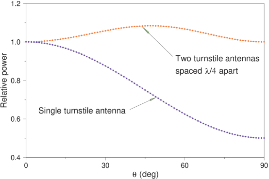
Figure 6: The relative radiation pattern of a single turnstile antenna, and of a pair of turnstile antennas that are separated by $\lambda/4$.

But we can make the pattern even more isotropic by considering a vertical stack of turnstile antennas.

If the center of the turnstile antenna had been at height $z$ along the $z$-axis, the only difference in the resulting electric and magnetic fields would be a phase change by $kz\cos\theta$ because the path length to the distant observer differs by $z\cos\theta$. That is, the fields (17)-(19) would simply be multiplied by the phase factor $e^{-ikz\cos\theta}$.

Thus, if we have two turnstile antennas, one whose center is at the origin, and the other whose center is at height $z$, and we operated them in phase, the fields (17)-(19) would be multiplied by

$$1+e^{-ikz\cos\theta}.$$ (22)

The radiated power would therefore by eq. (21) multiplied by the absolute square of eq. (22):

$${dP\over d\Omega}=2{p_{0}^{2}\omega^{4}\over 8\pi c^{3}}(1+\cos^{2}\theta)[1+\cos(kz\cos\theta)].$$ (23)

For example, suppose $kz=\pi/2$, i.e., the vertical separation of the two antennas is 1/4 of a wavelength. Then, the peak of the radiation pattern is only 1.08 times (0.35 db) greater than the minimum, as shown in Fig. 6. For most practical purposes, this double turnstile antenna could be considered to be isotropic.

Saunders [3] has further shown that an infinite array of turnstile antennas yields strictly isotropic radiation provided the number $N(z)$ of such antennas in an interval $dz$ along the vertical axis is proportional to $K_{0}(kz)$, the so-called modified Bessel function of order zero [9], whose behavior is sketched in Fig. 7. The antennas are all driven in phase. Since the function $K_{0}(kz)$ is sharply peaked at $z=0$, we see that a properly spaced collection of turnstile antennas that extends over only $\pm 1$ wavelength in $z$ could produce an extremely isotropic radiation pattern.

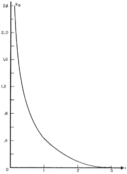
Figure 7: The modified Bessel function $K_{0}(x)$. From [9].

The U-shaped antenna of sec. 2 is a variant on the theme of a vertical stack of turnstile antennas. Since the currents are opposite in the two vertical arms of the U-shaped antenna, the charge accumulations on these arms have opposite signs as well. Thus, the two vertical arms are in effect a vertical stack of horizontal dipole antennas. If we had a second U-shaped antenna, rotated by 90^∘ about the vertical compared to the first, and driven $90^{\circ}$ out of phase, this would be equivalent to a vertical stack of (horizontal) turnstile antennas. Such a double U-shaped antenna is discussed in sec. 6.5.2 of [5], where its radiation pattern is found to be isotropic, although the details of the polarization of the radiation fields differ slightly from those for a single U-shaped radiator.

References

- [1] L.E.J. Brouwer, On Continuous Vector Distributions on Surfaces, Proc. Royal Acad. (Amsterdam) 11, 850 (1909); Collected Works, Volume 2: Geometry, Analysis, Topology, and Mechanics, ed. by Hans Freudenthal (North-Holland Publishing Company, 1976), p. 301.
- [2] H.F. Mathis, A short proof that an isotropic antenna is impossible, Proc. I.R.E. 39, 970 (1951); On isotropic antennas, Proc. I.R.E. 42, 1810 (1954).
- [3] W.K. Saunders, On the Unity Gain Antenna, in Electromagnetic Theory and Antennas, ed. by E.C. Jordan (Pergamon Press, New York, 1963), Vol. 2, p. 1125.
- [4] H. Matzner, M. Milgrom and S. Shtrikman, Magnetoelectric Symmetry and Electromagnetic Radiation, Ferroelectrics 161, 213 (1994).
- [5] H. Matzner, Moment Method and Microstrip Antennas, Ph.D. Thesis (Weizmann Institute of Science, Rehovot, Israel, 1993).
- [6] See, for example, eq. (14-53) of W.K.H. Panofsky and M. Phillips, Classical Electricity and Magnetism, 2nd ed. (Addison-Wesley, Reading, MA, 1962).
- [7] G.H. Brown, The “Turnstile” Antenna, Electronics 9, 15 (April, 1936).
- [8] L.B. Cebik, The Turnstile Antenna. An Omni-Directional Horizontally Polarized Antenna, http://www.cebik.com/turns.html
- [9] M. Abramowitz and I. Stegun, Handbook of Mathematical Functions (National Bureau of Standards, Washington, D.C., 1964), sec. 9.6.