1 Problem

Gaussian beams provide the simplest mathematical description of the essential features of a focused optical beam, by ignoring higher-order effects induced by apertures elsewhere in the system.

Wavefunctions $\psi({\bf x},t)=\psi({\bf x})e^{-i\omega t}$ for Gaussian laser beams [1, 2, 3, 4, 5, 6, 7, 10, 11, 12] of angular frequency $\omega$ are typically deduced in the paraxial approximation, meaning that in the far zone the functions are accurate only for angles $\theta$ with respect to the beam axis that are at most a few times the characteristic diffraction angle

$$\theta_{0}={\lambda\over\pi w_{0}}={2\over kw_{0}}={w_{0}\over z_{0}}\,,$$ (1)

where $\lambda$ is the wavelength, $k=\omega/c=2\pi/\lambda$ is the wave number, $c$ is the speed of light, $w_{0}$ is the radius of the beam waist, and $z_{0}$ is the depth of focus, also called the Rayleigh range, which is related by

$$z_{0}={kw_{0}^{2}\over 2}={2\over k\theta_{0}^{2}}\,.$$ (2)

Since the angle with respect to the beam axis has unique meaning only up to a value of $\pi/2$, the paraxial approximation implies that $\theta_{0}\ll 1$, and consequently that $z_{0}\gg w_{0}\gg\lambda$.

The question arises whether there are any “exact” solutions to the free-space wave equation

$$\nabla^{2}\psi-{1\over c^{2}}{\partial^{2}\psi\over\partial t^{2}}=0,$$ (3)

for which the paraxial wavefunctions are a suitable approximation. For monochromatic waves, it suffices to seek “exact” solutions to the Helmholtz wave equation,

$$\nabla^{2}\psi+k^{2}\psi=0.$$ (4)

This equation is known to be separable in 11 coordinate systems [13, 14], of which oblate spheroidal coordinates are well matched to the geometry of laser beams, as shown in Fig. 1.

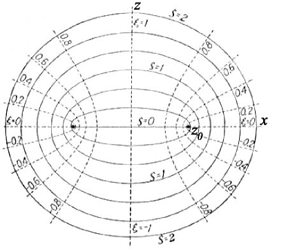
Figure 1: The $x$-$z$ plane of an oblate spheroidal coordinate system $({\small{\raise 2.0pt\hbox{$\zeta$}}},\xi,\phi)$ based on hyperboloids and ellipsoids of revolution about the $z$ axis, with foci at $(x,z)=(\pm z_{0},0)$. The coordinates have ranges $0\leq{\small{\raise 2.0pt\hbox{$\zeta$}}}<\infty$, $-1\leq\xi\leq 1$, and $0\leq\phi\leq 2\pi)$.

“Exact” solutions to the Helmholtz equation in oblate spheroidal coordinates were developed in the 1930’s, and are summarized in [15, 16, 17]. These solutions are, however, rather intricate and were almost forgotten at the time of the invention of the laser in 1960 [18].

This problem does not explore the “exact” solutions, but rather asks you to develop a systematic set of approximate solutions to the Helmholtz equation in oblate spheroidal coordinates, which will turn out to be one representation of paraxial Gaussian laser beams.

The relation between rectangular coordinates $(x,y,z)$ and oblate spheroidal coordinates $({\small{\raise 2.0pt\hbox{$\zeta$}}},\xi,\phi)$ is

$$x = z_{0}\sqrt{1+{\small{\raise 2.0pt\hbox{$\zeta$}}}^{2}}\sqrt{1-\xi^{2}}\cos\phi,$$ (5)

$$y = z_{0}\sqrt{1+{\small{\raise 2.0pt\hbox{$\zeta$}}}^{2}}\sqrt{1-\xi^{2}}\sin\phi,$$ (6)

$$z = z_{0}{\small{\raise 2.0pt\hbox{$\zeta$}}}\xi,$$ (7)

where the length $z_{0}$ is the distance from the origin to one of the foci of the ellipses and hyperbolae whose surfaces of revolution about the $z$ axis are surfaces of constant $\zeta$ and $\xi$. Coordinate $\phi$ is the usual azimuthal angle measured in the $x$-$y$ plane. For large $\zeta$, the oblate spheroidal coordinates are essentially identical to spherical coordinates $(r,\theta,\phi)$ with the identification ${\small{\raise 2.0pt\hbox{$\zeta$}}}=r/z_{0}$ and $\xi=\cos\theta$.

An obvious consequence of the definitions (5)-(7) is that

$$r_{\perp}=\sqrt{x^{2}+y^{2}}=z_{0}\sqrt{1+{\small{\raise 2.0pt\hbox{$\zeta$}}}^{2}}\sqrt{1-\xi^{2}}.$$ (8)

It is clear that the oblate spheroidal wave functions will have the mathematical restriction that the entire wave crosses the plane $z=0$ within an iris of radius $z_{0}$, the length used in the definitions (5)-(7) of the oblate spheroidal coordinates. In effect, the plane $z=0$ is perfectly absorbing except for the iris of radius $z_{0}$.

You will find that the length $z_{0}$ also has the physical significance of the Rayleigh range, which concept is usually associated with longitudinal rather than tranverse behavior of the waves. Since the paraxial approximation that you will explore is valid only when the beam waist $w_{0}$ is small compared to the Rayleigh range, i.e., when $w_{0}\ll z_{0}$, the paraxial wave functions are not accurate descriptions of waves of extremely short focal length, even though they will be formally defined for any value of $w_{0}$.

The wave equation (4) is separable in oblate spheroidal coordinates, with the form

$${\partial\over\partial{\small{\raise 2.0pt\hbox{$\zeta$}}}}(1+{\small{\raise 2.0pt\hbox{$\zeta$}}}^{2}){\partial\psi\over\partial{\small{\raise 2.0pt\hbox{$\zeta$}}}}+{\partial\over\partial\xi}(1-\xi^{2}){\partial\psi\over\partial\xi}+{{\small{\raise 2.0pt\hbox{$\zeta$}}}^{2}+\xi^{2}\over(1+{\small{\raise 2.0pt\hbox{$\zeta$}}}^{2})(1-\xi^{2})}{\partial^{2}\psi\over\partial\phi^{2}}+k^{2}z_{0}^{2}({\small{\raise 2.0pt\hbox{$\zeta$}}}^{2}+\xi^{2})\psi=0.$$ (9)

It is helpful to express the wave functions in radial and transverse coordinates that are scaled by the Rayleigh range $z_{0}$ and by the diffraction angle $\theta_{0}$, respectively. The oblate spheroidal coordinate $\zeta$ already has this desirable property for large values. However, the coordinate $\xi$ is usefully replaced by

$$\sigma={1-\xi^{2}\over\theta_{0}^{2}}={z_{0}^{2}\over w_{0}^{2}}(1-\xi^{2})={kz_{0}\over 2}(1-\xi^{2})={r_{\perp}^{2}\over w_{0}^{2}(1+{\small{\raise 2.0pt\hbox{$\zeta$}}}^{2})}\,,$$ (10)

which obeys $\sigma\approx(\theta/\theta_{0})^{2}$ for large $r$ and small $\theta$, and $\sigma\approx(r_{\perp}/w_{0})^{2}$ near the beam waist where ${\small{\raise 2.0pt\hbox{$\zeta$}}}\approx 0$.

To replace $\xi$ by $\sigma$ in the Helmholtz equation (9), note that $2\xi d\xi=-\theta_{0}^{2}d\sigma$. In the paraxial approximation, $\xi\approx 1$ (which implies that your solution will be restricted to waves in the hemisphere $z\geq 0$), you may to suppose that

$$d\xi\approx-{\theta_{0}^{2}\over 2}d\sigma.$$ (11)

Find an orthogonal set of waves,

$$\psi_{n}^{m}=Z_{n}^{m}({\small{\raise 2.0pt\hbox{$\zeta$}}})S_{n}^{m}(\sigma)e^{\pm im\phi},$$ (12)

which satisfy the Helmholtz equation in the paraxial approximation. You may anticipate that the “angular” functions $S_{n}^{m}(\sigma)$ are modulated Gaussians, containing a factor $\sigma^{m/2}e^{-\sigma}$. The “radial” functions $Z_{n}^{m}$ are modulated spherical waves in the far zone, with a leading factor $e^{ikr}$, and it suffices to keep terms in the remaining factor that are lowest order in the small quantity $\theta_{0}$.

Vector electromagnetic waves ${\bf E}={\bf E}({\bf x})e^{-i\omega t}$ and ${\bf B}={\bf B}({\bf x})e^{-i\omega t}$ that satisfy Maxwell’s equations in free space can be generated from the scalar wave functions $\psi_{n}^{m}$ by supposing the vector potential A has Cartesian components (for which $(\nabla^{2}{\bf A})_{j}=\nabla^{2}A_{j}$ [14]) given by one or more of the scalar waves $\psi_{n}^{m}e^{-i\omega t}$. For these waves, the fourth Maxwell equation in free space is $c\nabla\times{\bf B}=\partial{\bf E}/\partial t=-ik{\bf E}$ (Gaussian units), so both fields E and B can de derived from the vector potential A according to,

$${\bf E}={i\over k}\nabla\times{\bf B}=ik{\bf A}+{i\over k}\nabla(\nabla\cdot{\bf A}),\qquad{\bf B}=\nabla\times{\bf A},$$ (13)

since the vector potential obeys the Helmholtz equation (4).

Calculate the ratio of the angular momentum density of the wave in the far zone to its energy density to show that quanta of these waves (photons with intrinsic spin $S=1$) carry orbital angular momentum in addition to the intrinsic spin. Show also that lines of the Poynting flux form spirals on a cone in the far zone.

2 Solution

2.1 The Paraxial Gaussian-Laguerre Wave Functions

Using the approximation (11) when replacing variable $\xi$ by $\sigma$, the Helmholtz equation (9) becomes

$${\partial\over\partial{\small{\raise 2.0pt\hbox{$\zeta$}}}}(1+{\small{\raise 2.0pt\hbox{$\zeta$}}}^{2}){\partial\psi\over\partial{\small{\raise 2.0pt\hbox{$\zeta$}}}}+{4\over\theta_{0}^{2}}{\partial\over\partial\sigma}\sigma{\partial\psi\over\partial\sigma}+{1+{\small{\raise 2.0pt\hbox{$\zeta$}}}^{2}-\theta_{0}^{2}\sigma\over(1+{\small{\raise 2.0pt\hbox{$\zeta$}}}^{2})\theta_{0}^{2}\sigma}{\partial^{2}\psi\over\partial\phi^{2}}+{4\over\theta_{0}^{4}}(1+{\small{\raise 2.0pt\hbox{$\zeta$}}}^{2}-\theta_{0}^{2}\sigma)\psi=0.$$ (14)

This equation admits separated solutions of the form (12) for any integer $m$. Inserting this in eq. (14) and dividing by $\psi$, we find

$${1\over Z}{\partial\over\partial{\small{\raise 2.0pt\hbox{$\zeta$}}}}(1+{\small{\raise 2.0pt\hbox{$\zeta$}}}^{2}){\partial Z\over\partial{\small{\raise 2.0pt\hbox{$\zeta$}}}}+{4\over\theta_{0}^{2}S}{\partial\over\partial\sigma}\sigma{\partial S\over\partial\sigma}-m^{2}{1+{\small{\raise 2.0pt\hbox{$\zeta$}}}^{2}-\theta_{0}^{2}\sigma\over(1+{\small{\raise 2.0pt\hbox{$\zeta$}}}^{2})\theta_{0}^{2}\sigma}+{4\over\theta_{0}^{4}}(1+{\small{\raise 2.0pt\hbox{$\zeta$}}}^{2})-{4\sigma\over\theta_{0}^{2}}=0.$$ (15)

The functions $Z$ and $S$ will be the same for integers $m$ and $-m$, so henceforth we consider $m$ to be non-negative, and write the azimuthal functions as $e^{\pm im\phi}$. With $\lambda_{m}$ as the second separation constant, the $\zeta$ and $\sigma$ differential equations are

$${d\over d{\small{\raise 2.0pt\hbox{$\zeta$}}}}(1+{\small{\raise 2.0pt\hbox{$\zeta$}}}^{2}){dZ\over d{\small{\raise 2.0pt\hbox{$\zeta$}}}} = \left(\lambda_{m}-{4\over\theta_{0}^{4}}(1+{\small{\raise 2.0pt\hbox{$\zeta$}}}^{2})-{m^{2}\over 1+{\small{\raise 2.0pt\hbox{$\zeta$}}}^{2}}\right)Z,$$ (16)

$${d\over d\sigma}\sigma{dS\over d\sigma} = -{\theta_{0}^{2}\over 4}\left(\lambda_{m}-{4\sigma\over\theta_{0}^{2}}-{m^{2}\over\theta_{0}^{2}\sigma}\right)S.$$ (17)

The hint is that the wave functions have Gaussian transverse dependence, which implies that the “angular” function $S(\sigma)$ contains a factor $e^{-\sigma}=e^{-r_{\perp}^{2}/w_{0}^{2}(1+{\tiny{\raise 2.0pt\hbox{$\zeta$}}}^{2})}$. We therefore write $S=e^{-\sigma}T$, and eq. (17) becomes

$$\sigma{d^{2}T\over d\sigma^{2}}+(1-2\sigma){dT\over d\sigma}+\left(1+{\theta_{0}^{2}\over 4}\lambda_{m}-{m^{2}\over 4\sigma}\right)T=0.$$ (18)

The function $T(\sigma)$ cannot be represented as a polynomial, but (like the radial Shrödinger equation) this can be accomplished after a factor of $\sigma^{m/2}$ is extracted. That is, we write $T=\sigma^{m/2}L$, or $S=\sigma^{m/2}e^{-\sigma}L$, so that eq. (18) becomes

$$\sigma{d^{2}L\over d\sigma^{2}}+(m+1-2\sigma){dL\over d\sigma}+\nu L=0,$$ (19)

where

$$\nu={\theta_{0}^{2}\over 4}\lambda_{m}-m-1.$$ (20)

If $\nu=2n$ for integer $n\geq 0$, this is the differential equation for generalized Laguerre polynomials $L_{n}^{m}(2\sigma)$ [19], where

$$L_{n}^{m}(x)=m!n!\sum_{k=0}^{n}{(-1)^{k}x^{k}\over(m+k)!(n-k)!k!}=1-{nx\over m+1}+{n(n-1)x^{2}\over 2(m+1)(m+2)}-...$$ (21)

By direct calculation from eq. (19) with $\nu=2n$, we readily verify that the low-order solutions are

$$L_{0}^{m}=1,\qquad L_{1}^{m}(2\sigma)=1-{2\sigma\over m+1}\,,\qquad L_{2}^{m}(2\sigma)=1-{4\sigma\over m+1}+{4\sigma^{2}\over(m+1)(m+2)}\,.$$ (22)

The Laguerre polynomials are normalized to 1 at $x=0$, and obey the orthogonality relation

$$\int_{0}^{\infty}L_{n}^{m}(x)L_{n^{\prime}}^{m}(x)x^{m}e^{-x}dz={(m!)^{2}n!\over(m+n)!}\delta_{nn^{\prime}}.$$ (23)

The “angular” functions $S_{n}^{m}(\sigma)$ are thus given by

$$S_{n}^{m}(\sigma)=\sigma^{m/2}e^{-\sigma}L_{n}^{m}(2\sigma),$$ (24)

which obey the orthogonality relation

$$\int_{0}^{\infty}S_{n}^{m}(\sigma)S_{n^{\prime}}^{m}(\sigma)d\sigma={1\over 2^{m+1}}\int_{0}^{\infty}L_{n}^{m}(x)L_{n^{\prime}}^{m}(x)x^{m}e^{-x}dz={(m!)^{2}n!\over(m+n)!2^{m+1}}\delta_{nn^{\prime}}.$$ (25)

In the present application, $0\leq\sigma\leq 1/\theta_{0}^{2}$, on which interval the functions $S_{n}^{m}$ are only approximately orthogonal. Because of the exponential damping of the $S_{n}^{m}$, their orthogonality is nearly exact for $\theta_{0}\mathrel{\vbox{\kern 0.0pt\hbox{$<$} \kern 0.0pt\hbox{$\sim$} }}1/2$.

We now turn to the “radial” functions $Z_{n}^{m}({\small{\raise 2.0pt\hbox{$\zeta$}}})$ which obey the differential equation (16) with separation constant $\lambda_{m}$ given by

$$\lambda_{m}={4\over\theta_{0}^{2}}(2n+m+1),$$ (26)

using eq. (20) with $\nu=2n$. For large $r$ the radial functions are essentially spherical waves, and hence have leading dependence $e^{ikr}$. For small polar angles, where $\xi\approx 1$, the relation (7) implies that $r\approx z_{0}{\small{\raise 2.0pt\hbox{$\zeta$}}}$, and $kr\approx kz_{0}{\small{\raise 2.0pt\hbox{$\zeta$}}}=2{\small{\raise 2.0pt\hbox{$\zeta$}}}/\theta_{0}^{2}$, recalling eq. (2). Hence we expect the radial functions to have the form

$$Z({\small{\raise 2.0pt\hbox{$\zeta$}}})=e^{2i{\tiny{\raise 2.0pt\hbox{$\zeta$}}}/\theta_{0}^{2}}F({\small{\raise 2.0pt\hbox{$\zeta$}}}).$$ (27)

Inserting this in eq. (16), we find that function $F$ obeys the second-order differential equation

$$\left(1+{\small{\raise 2.0pt\hbox{$\zeta$}}}^{2}\right)\left({d^{2}F\over d{\small{\raise 2.0pt\hbox{$\zeta$}}}^{2}}+{4i\over\theta_{0}^{2}}{dF\over d{\small{\raise 2.0pt\hbox{$\zeta$}}}}\right)+2{\small{\raise 2.0pt\hbox{$\zeta$}}}\left({dF\over d{\small{\raise 2.0pt\hbox{$\zeta$}}}}+{2iF\over\theta_{0}^{2}}\right)=\left({4\over\theta_{0}^{2}}(2n+m+1)-{m^{2}\over 1+{\small{\raise 2.0pt\hbox{$\zeta$}}}^{2}}\right)F.$$ (28)

In the paraxial approximation, $\theta_{0}$ is small, so we keep only those terms in eq. (28) that vary as $1/\theta_{0}^{2}$, which yields the first-order differential equation,

$$\left(1+{\small{\raise 2.0pt\hbox{$\zeta$}}}^{2}\right){dF\over d{\small{\raise 2.0pt\hbox{$\zeta$}}}}=-\left({\small{\raise 2.0pt\hbox{$\zeta$}}}+i(2n+m+1)\right)F.$$ (29)

For $m=n=0$ we write $F_{0}^{0}=f$, in which case eq. (29) reduces to

$$\left(1+{\small{\raise 2.0pt\hbox{$\zeta$}}}^{2}\right){df\over d{\small{\raise 2.0pt\hbox{$\zeta$}}}}=\left({\small{\raise 2.0pt\hbox{$\zeta$}}}+i\right)\left({\small{\raise 2.0pt\hbox{$\zeta$}}}-i\right){df\over d{\small{\raise 2.0pt\hbox{$\zeta$}}}}=-\left({\small{\raise 2.0pt\hbox{$\zeta$}}}+i\right)f,$$ (30)

or

$${df\over f}=-{d{\small{\raise 2.0pt\hbox{$\zeta$}}}\over{\small{\raise 2.0pt\hbox{$\zeta$}}}-i}\,.$$ (31)

This integrates to $\ln f=\ln C-\ln\left({\small{\raise 2.0pt\hbox{$\zeta$}}}-i\right)$. We define $f(0)=1$, so that $C=-i$ and

$$f={1\over 1+i{\small{\raise 2.0pt\hbox{$\zeta$}}}}={1-i{\small{\raise 2.0pt\hbox{$\zeta$}}}\over 1+{\small{\raise 2.0pt\hbox{$\zeta$}}}^{2}}={e^{-i\tan^{-1}{\tiny{\raise 2.0pt\hbox{$\zeta$}}}}\over\sqrt{1+{\small{\raise 2.0pt\hbox{$\zeta$}}}^{2}}}\,.$$ (32)

At large $\zeta$, $f\approx 1/{\small{\raise 2.0pt\hbox{$\zeta$}}}\propto 1/r$, as expected in the far zone for waves that have a narrow waist at $z=0$. Indeed, we expect that $F_{n}^{m}\propto 1/{\small{\raise 2.0pt\hbox{$\zeta$}}}$ at large $\zeta$ for all $m$ and $n$. This suggests that $F_{n}^{m}$ differs from $f$ by only a phase change. A suitable form is

$$F_{n}^{m}={e^{-ia_{m,n}\tan^{-1}{\tiny{\raise 2.0pt\hbox{$\zeta$}}}}\over\sqrt{1+{\small{\raise 2.0pt\hbox{$\zeta$}}}^{2}}}={\left(e^{-i\tan^{-1}{\tiny{\raise 2.0pt\hbox{$\zeta$}}}}\right)^{a_{m,n}}\over\sqrt{1+{\small{\raise 2.0pt\hbox{$\zeta$}}}^{2}}}={1\over\sqrt{1+{\small{\raise 2.0pt\hbox{$\zeta$}}}^{2}}}\left({1-i{\small{\raise 2.0pt\hbox{$\zeta$}}}\over\sqrt{1+{\small{\raise 2.0pt\hbox{$\zeta$}}}^{2}}}\right)^{a_{m,n}}={\left(1-i{\small{\raise 2.0pt\hbox{$\zeta$}}}\right)^{a_{m,n}}\over\left(1+{\small{\raise 2.0pt\hbox{$\zeta$}}}^{2}\right)^{(1+a_{m,n})/2}}\,.$$ (33)

Inserting this hypothesis in the differential equation (29), we find that it is satisfied provided

$$a_{m,n}=2n+m+1.$$ (34)

Thus, the radial function is

$$Z_{n}^{m}({\small{\raise 2.0pt\hbox{$\zeta$}}})=e^{ikz_{0}{\tiny{\raise 2.0pt\hbox{$\zeta$}}}}F_{n}^{m}={e^{i[kz_{0}{\tiny{\raise 2.0pt\hbox{$\zeta$}}}-(2n+m+1)\tan^{-1}{\tiny{\raise 2.0pt\hbox{$\zeta$}}}]}\over\sqrt{1+{\small{\raise 2.0pt\hbox{$\zeta$}}}^{2}}}\,,$$ (35)

and the paraxial Gaussian-Laguerre wave functions are

$$\psi_{n}^{m}(\sigma,\phi,{\small{\raise 2.0pt\hbox{$\zeta$}}},t)=Z_{n}^{m}S_{n}^{m}e^{\pm im\phi}e^{-i\omega t}={\sigma^{m/2}e^{-\sigma}L_{n}^{m}(2\sigma)e^{i[kz_{0}{\tiny{\raise 2.0pt\hbox{$\zeta$}}}-\omega t-(2n+m+1)\tan^{-1}{\tiny{\raise 2.0pt\hbox{$\zeta$}}}\pm m\phi]}\over\sqrt{1+{\small{\raise 2.0pt\hbox{$\zeta$}}}^{2}}}\,.$$ (36)

The factor $e^{-i(2n+m+1)\tan^{-1}{\tiny{\raise 2.0pt\hbox{$\zeta$}}}}$ in the wave functions implies a phase shift of $(2n+m+1)\pi/2$ between the focal plane and the far field, as first noticed by Guoy [20] for whom this effect is named. Even the lowest mode, with $m=n=0$, has a Guoy phase shift of $\pi/2$. This phase shift is an essential difference between a plane wave and a wave that is asymptotically plane but which has emerged from a focal region. The existence of this phase shift can be deduced from an elementary argument that applies Faraday’s law to wave propagation through an aperture [21], as well as by arguments based on the Kirchhoff diffraction integral [10] as were used by Guoy.

It is useful to relate the coordinates $\sigma$ and $\zeta$ to those of a cylindrical coordinate system $(r_{\perp},\phi,z)$, in the paraxial approximation that $\xi\approx 1$. For this, we recall from eqs. (7), (8) and (10) that

$$\xi=1-\theta_{0}^{2}\sigma\approx 1,$$ (37)

so

$${\small{\raise 2.0pt\hbox{$\zeta$}}}^{2}={z^{2}\over z_{0}^{2}\xi^{2}}\approx{z^{2}\over z_{0}^{2}}(1+\theta_{0}^{2}\sigma),$$ (38)

and hence,

$$r_{\perp}^{2}=w_{0}^{2}\sigma(1+{\small{\raise 2.0pt\hbox{$\zeta$}}}^{2})\approx w_{0}^{2}\sigma\left(1+{z^{2}\over z_{0}^{2}}\right)+\theta_{0}^{4}\sigma z^{2}\approx w_{0}^{2}\sigma\left(1+{z^{2}\over z_{0}^{2}}\right),$$ (39)

where we neglect terms in $\theta_{0}^{4}$ in the lowest-order paraxial approximation. Then,

$$\sigma\approx{r_{\perp}^{2}\over w_{0}^{2}(1+z^{2}/z_{0}^{2})}\,,$$ (40)

and

$${\small{\raise 2.0pt\hbox{$\zeta$}}}\approx{z\over z_{0}}\left(1+{\theta_{0}^{2}\sigma\over 2}\right)\approx{z\over z_{0}}\left(1+{\theta_{0}^{2}r_{\perp}^{2}\over 2w_{0}^{2}(1+z^{2}/z_{0}^{2})}\right)={z\over z_{0}}\left(1+{r_{\perp}^{2}\over 2(z^{2}+z_{0}^{2})}\right).$$ (41)

For large $z$ eq. (41) becomes

$${\small{\raise 2.0pt\hbox{$\zeta$}}}\approx{z\over z_{0}}\left(1+{r_{\perp}^{2}\over 2z^{2}}\right)\approx{z\over z_{0}}\sqrt{1+{r_{\perp}^{2}\over z^{2}}}={r\over z_{0}}\,,$$ (42)

as expected. That is, the factor $e^{i(kz_{0}{\tiny{\raise 2.0pt\hbox{$\zeta$}}}-\omega t)}$ in the wave functions (36) implies that they are spherical waves in the far zone.

The characteristic transverse extent of the waves at position $z$ is sometimes called $w(z)$. From eq. (40) we see that the Gaussian behavior $e^{-\sigma}$ of the angular functions implies that

$$w(z)=w_{0}\sqrt{1+{z^{2}\over z_{0}^{2}}}\,.$$ (43)

The paraxial approximation is often taken to mean that variable $\zeta$ is simply $z/z_{0}$ everywhere in eq. (36) except in the phase factor $e^{ikz_{0}{\tiny{\raise 2.0pt\hbox{$\zeta$}}}}$, where the form (41) is required so that the waves are spherical in the far zone. In this convention, we can write

$$\psi_{n}^{m}(r_{\perp},\phi,z,t)={\sigma^{m/2}e^{-\sigma}L_{n}^{m}(2\sigma)e^{i\{kz[1+r_{\perp}^{2}/2(z^{2}+z_{0}^{2})]-\omega t-(2n+m+1)\tan^{-1}(z/z_{0})\pm m\phi\}}\over\sqrt{1+z^{2}/z_{0}^{2}}}\,.$$ (44)

The wave functions may be written in a slightly more compact form if we use the scaled coordinates

$$\rho={r_{\perp}\over w_{0}}\,,\qquad{\small{\raise 2.0pt\hbox{$\zeta$}}}={z\over z_{0}}\,,\qquad\sigma={\rho^{2}\over 1+{\small{\raise 2.0pt\hbox{$\zeta$}}}^{2}}\,.$$ (45)

Then, the simplest wave function is

$$\psi_{0}^{0}(r_{\perp},\phi,z,t) = e^{-\rho^{2}/(1+{\tiny{\raise 2.0pt\hbox{$\zeta$}}}^{2})}e^{ikzr_{\perp}^{2}/2z_{0}^{2}(1+{\tiny{\raise 2.0pt\hbox{$\zeta$}}}^{2})}e^{i(kz-\omega t)}{e^{-i\tan^{-1}{\tiny{\raise 2.0pt\hbox{$\zeta$}}}}\over\sqrt{1+{\small{\raise 2.0pt\hbox{$\zeta$}}}^{2}}}$$ (46)

$$= fe^{-\rho^{2}(1-i{\tiny{\raise 2.0pt\hbox{$\zeta$}}})/(1+{\tiny{\raise 2.0pt\hbox{$\zeta$}}}^{2})}e^{i(kz-\omega t)}=fe^{-f\rho^{2}}e^{i(kz-\omega t)},$$

recalling eq. (2) and the definition of $f({\small{\raise 2.0pt\hbox{$\zeta$}}})$ in eq. (32). In this manner the general, paraxial wave function can be written

$$\psi_{n}^{m}(r_{\perp},\phi,z,t)=f^{m+1}\rho^{m}e^{-f\rho^{2}}L_{n}^{m}(2\sigma)e^{i(kz-\omega t\pm m\phi-2n\tan^{-1}{\tiny{\raise 2.0pt\hbox{$\zeta$}}})}.$$ (47)

It is noteworthy that although our solution began with the hypothesis of separation of variables in oblate spheroidal coordinates, we have found wave functions that contain the factors $e^{-f\rho^{2}}$ and $L_{n}^{m}(\sigma)$ that are nonseparable functions of $r_{\perp}$ and $z$ in cylindrical coordinates.

The wave functions found above are for a pure frequency $\omega$. In practice one is often interested in pulses of characteristic width $\tau$ whose frequency spectrum is centered on frequency $\omega$. In this case we can replace the factor $e^{i(kz-\omega t)}$ in the wave function by $g(\varphi)e^{i\varphi}$, where the phase is $\varphi=kz-\omega t$, and still satisfy the wave equation (3) provided that the modulation factor $g$ obeys [11]

$$\left|g^{\prime}\over g\right|\ll 1.$$ (48)

An important example of a pulse shape that satisfies eq. (48) is

$$g(\varphi)={\rm sech}{\varphi\over\omega\tau}\,,$$ (49)

so long as $\omega\tau\gg 1$, i.e., so long as the pulse is longer that a few periods of the carrier wave. Perhaps surprisingly, a Gaussian temporal profile is not consistent with condition (48). Hence, a “Gaussian beam” can have a Gaussian transverse profile, but not a Gaussian longitudinal profile as well.

2.2 Electric and Magnetic Fields of Gaussian Beams

The scalar wave functions (47) can be used to generate vector electromagnetic fields that satisfy Maxwell’s equations. For this, we use eqs. (13) with a vector potential A whose Cartesian components are one or more of the functions (47).

If we wish to express the electromagnetic fields in cylindrical coordinates, then we immediately obtain one family of fields from the vector potential

$$A_{x}=A_{y}=A_{\perp}=A_{\phi}=0,\qquad A_{z}={E_{0}\over k\theta_{0}}\psi_{n}^{m}(r_{\perp},\phi,z,t).$$ (50)

The resulting magnetic field has no $z$ component, so we may call these transverse magnetic (TM) waves. If index $m=0$ then A has no $\phi$ dependence, and the magnetic field has no radial component; the magnetic field lines are circles about the $z$ axis.

The lowest-order TM mode, corresponding to indices $m=n=0$, has field components

$$E_{\perp} = E_{0}\rho f^{2}e^{-f\rho^{2}}ge^{i\varphi}+{\cal O}(\theta_{0}^{2}),$$

$$E_{\phi} = 0,$$

$$E_{z} = i\theta_{0}E_{0}f^{2}(1-f\rho^{2})e^{-f\rho^{2}}ge^{i\varphi}+{\cal O}(\theta_{0}^{3}).$$

$$B_{\perp} = 0,$$

$$B_{\phi} = E_{\perp},$$

$$B_{z} = 0,$$ (51)

as apparently first deduced in [22]. This is a so-called axicon mode [11], in which the electric field is dominantly radial, which component necessarily vanishes along the beam axis. In the far zone the beam intensity is largest on a cone of half angle $\theta_{0}$ and is very small on the axis itself; the beam appears to have a hole in the center.

The radial and longitudinal electric field of the TM${}_{0}^{0}$ mode are illustrated in Figs. 2 and 3. Photographs of Gaussian-Laguerre laser modes from [23] are shown in Fig. 4.

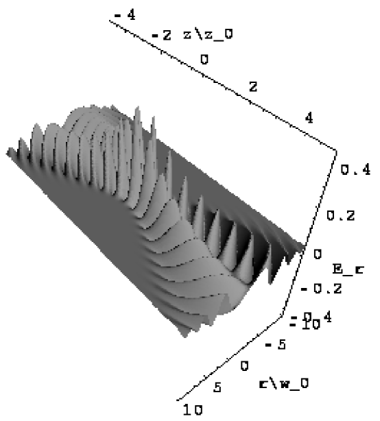
Figure 2: The electric field $E_{r}(r_{\perp},0,z)$ of the TM${}_{0}^{0}$ axicon Gaussian beam with diffraction angle $\theta_{0}=0.45$, according to eq. (51).

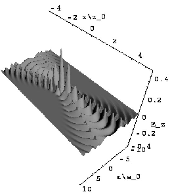
Figure 3: The electric field $E_{z}(r_{\perp},0,z)$ of the TM${}_{0}^{0}$ axicon Gaussian beam with diffraction angle $\theta_{0}=0.45$, according to eq. (51).

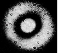
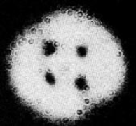
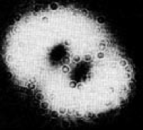
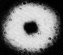
Figure 4: Photographs of Gaussian-Laguerre laser beams with $2n+m=2$. From [23].

As is well known, corresponding to each TM wave solution to Maxwell’s equations in free space, there is a TE (transverse electric) mode obtained by the duality transformation

$${\bf E}_{\rm TE}={\bf B}_{\rm TM},\qquad{\bf B}_{\rm TE}=-{\bf E}_{\rm TM}.$$ (52)

Since we are considering waves in free space where $\nabla\cdot{\bf E}=0$, the electric field could also be deduced from a vector potential, and the magnetic field from the electric field, according to the dual of eq. (13),

$${\bf E}=\nabla\times{\bf A},\qquad{\bf B}=-{i\over k}\nabla\times{\bf E}.$$ (53)

Then, the TE modes can be obtained by use of the vector potential (50) in eq. (53).

The TM Gaussian-Laguerre modes emphasize radial polarization of the electric field, and the TE modes emphasize circular polarization. In many physical applications, linear polarization is more natural, for which the modes are well-described by Gaussian-Hermite wave functions [2, 3, 4, 8]. Formal transformations between the Gaussian-Hermite wave functions and the Gaussian-Laguerre functions have been described in [24].

2.3 Energy, Momentum and Angular Momentum in the Far Zone

The electromagnetic field energy density,

$$u={E^{2}+B^{2}\over 8\pi}\,,$$ (54)

the field momentum density,

$${\bf p}={{\bf E}\times{\bf B}\over 4\pi c}\,,$$ (55)

and the field angular momentum density,

$${\bf l}={\bf r}\times{\bf p},$$ (56)

are the same for a TM Gaussian-Laguerre mode and the TE mode related to it by the duality transformation (52).

We consider the energy, momentum and angular momentum for TM waves in the far zone, where ${\small{\raise 2.0pt\hbox{$\zeta$}}}\approx r/z_{0}\gg 1$, and $r_{\perp}\approx r\theta\ll r$ in terms of spherical coordinates $(r,\theta,\phi)$. Then the waves are nearly spherical, and so have a phase factor $e^{ikr}$ that implies the electric field is related to the magnetic field by

$${\bf E}={i\over k}\nabla\times{\bf B}\approx{\bf B}\times\hat{\bf r},$$ (57)

so that $E^{2}=B^{2}$. The time-averaged densities can therefore be written

$$\left\langle u\right\rangle={\left|B\right|^{2}\over 8\pi}\,,$$ (58)

$$\left\langle{\bf p}\right\rangle={Re[({\bf B}\times\hat{\bf r})\times{\bf B}^{\star}]\over 8\pi c}={\left|B\right|^{2}\hat{\bf r}-Re[({\bf B}\cdot\hat{\bf r}){\bf B}^{\star}]\over 8\pi c}\,,$$ (59)

and

$$\left\langle{\bf l}\right\rangle=-{Re[({\bf B}\cdot\hat{\bf r})({\bf r}\times{\bf B}^{\star})]\over 8\pi c}\,.$$ (60)

The TM waves are derived from the vector potential (50) whose only nonzero component is $A_{z}$. Then, the magnetic field components in cylindrical coordinates are

$$B_{\perp}={1\over r_{\perp}}{\partial A_{z}\over\partial\phi}={\pm imA_{z}\over r_{\perp}},\qquad B_{\phi}=-{\partial A_{z}\over\partial r_{\perp}}=-{1\over w_{0}}{\partial A_{z}\over\partial\rho},\qquad B_{z}=0,$$ (61)

where $\rho=r_{\perp}/w_{0}$. The radius vector r has cylindrical components $(r_{\perp},0,z)$, so

$${\bf B}\cdot\hat{\bf r}={B_{\perp}r_{\perp}\over r},\qquad\mbox{and}\qquad{\bf r}\times{\bf B}^{\star}=-\hat{\bf r}_{\perp}zB_{\phi}^{\star}+\hat{\phi}zB_{\perp}^{\star}+\hat{\bf z}r_{\perp}B_{\phi}^{\star}.$$ (62)

Only the $z$ component of the angular momentum can be nonzero for the beam as a whole, so we calculate

$$\left\langle l_{z}\right\rangle = -{r_{\perp}^{2}\over 8\pi cr}Re(B_{\perp}B_{\phi}^{\star})\approx{\pm m\over 8\pi cw_{0}}\theta Re\left(iA_{z}{\partial A_{z}^{\star}\over\partial\rho}\right)={\pm m\over 8\pi cw_{0}}{2\theta\over kw_{0}\theta_{0}}Re\left(iA_{z}{\partial A_{z}^{\star}\over\partial\rho}\right)$$ (63)

$$= {\pm m\over 4\pi\omega w_{0}^{2}}{\theta\over\theta_{0}}Re\left(iA_{z}{\partial A_{z}^{\star}\over\partial\rho}\right),$$

recalling that $r_{\perp}/r\approx\theta$ and $\theta_{0}=2/kw_{0}^{2}$. The factors of $A_{z}$ that depend on $r_{\perp}$ and $\sigma\approx z_{0}^{2}\rho^{2}/r^{2}$ are

$$A_{z}\propto\rho^{m}e^{-f\rho^{2}}L_{n}^{m}(2\sigma)\approx\rho^{m}e^{-f\rho^{2}}\left(1-{2nz_{0}^{2}\rho^{2}\over(m+1)r^{2}}\right),$$ (64)

where in the far zone, $f({\small{\raise 2.0pt\hbox{$\zeta$}}})\approx-iz_{0}/r$. Thus,

$${\partial A_{z}\over\partial\rho}\approx\left({m\over\rho^{2}}+2i{z_{0}\over r}-{4nz_{0}^{2}\over(m+1)r^{2}}\right)\rho A_{z}\approx 2i{z_{0}\over r}\rho A_{z}\approx 2i{\theta\over\theta_{0}}A_{z},$$ (65)

since in the far zone the factor $\rho^{m}e^{-f\rho^{2}}\approx\rho^{m}e^{-\rho^{2}/{\tiny{\raise 2.0pt\hbox{$\zeta$}}}^{2}}$ implies that the wave functions are large only for $\rho\approx\sqrt{m}\ {\small{\raise 2.0pt\hbox{$\zeta$}}}\approx\sqrt{m}\ r/z_{0}\gg 1$. Inserting this in eq. (63), we find

$$\left\langle l_{z}\right\rangle\approx{\pm m\over 2\pi\omega w_{0}^{2}}{\theta^{2}\over\theta_{0}^{2}}\left|A_{z}\right|^{2}.$$ (66)

To compare with the energy density, we need

$$\left|B\right|^{2}=\left|B_{\perp}\right|^{2}+\left|B_{\phi}\right|^{2}={m^{2}\over r_{\perp}^{2}}\left|A_{z}\right|^{2}+{1\over w_{0}^{2}}\left|\partial A_{z}\over\partial\rho\right|^{2}\approx{1\over w_{0}^{2}}\left({m^{2}\over\rho^{2}}+4{\theta^{2}\over\theta_{0}^{2}}\right)\left|A_{z}\right|^{2}\approx{4\over w_{0}^{2}}{\theta^{2}\over\theta_{0}^{2}}\left|A_{z}\right|^{2},$$ (67)

since $\rho=\pi r\theta_{0}/\lambda\theta\gg\theta_{0}/\theta$ in the far zone. Using this in eq. (58), we have

$$\left\langle u\right\rangle\approx{1\over 2\pi w_{0}^{2}}{\theta^{2}\over\theta_{0}^{2}}\left|A_{z}\right|^{2},$$ (68)

and the ratio of angular momentum density to energy density of a Gaussian-Laguerre mode is

$${\left\langle l_{z}\right\rangle\over\left\langle u\right\rangle}\approx{\pm m\over\omega}\,,$$ (69)

where the $\pm$ sign corresponds to azimuthal dependence $e^{\pm im\phi}$.

In a quantum view, the mode contains $N$ photons per unit volume of energy $\hbar\omega$ each, so the classical result (69) implies that each of these photons carries orbital angular momentum $\pm m\hbar$. Since the photons have intrinsic spin $S=1$, with $S_{z}=\pm 1$, we infer that the photons of a Gaussian-Laguerre mode carry total angular momentum component $J_{z}=\pm m\pm 1$.

The angular momentum of Gaussian-Laguerre modes has also been discussed in [25], in a slightly different approximation. The first macroscopic evidence for the angular momentum of light appears to have been given in [26].

Using the above relations we can evaluate to momentum density (59), which is proportional to the Poynting vector, and in the far zone we find

$$\left\langle{\bf p}\right\rangle\approx{\left\langle u\right\rangle\over c}\left(\hat{\bf r}\mp{m\over kr_{\perp}}\hat{\phi}\right)\approx{\left\langle u\right\rangle\over c}\left(\hat{\bf z}+\theta\hat{\bf r}_{\perp}\mp{m\over kr_{\perp}}\hat{\phi}\right).$$ (70)

Since $kr_{\perp}\gg 1$ in the far zone, the energy flow is largely radial outward from the focal region. The small azimuthal component causes the lines of energy flow to become spirals, which lie on cones of constant polar angle $\theta$ in the far zone

We can, of course, also deduce the angular momentum density $\left\langle l_{z}\right\rangle=[{\bf r}\times\left\langle{\bf p}\right\rangle]_{z}$ using eq. (70).

References

- [1] Paraxial Gaussian laser beams were introduced nearly simultaneously from two different approaches in [2] and [3]. An influential review article is [4]. Corrections to the paraxial approximation were first organized in a power series in the parameter in [5]. The understanding that the scalar, paraxial wave function is best thought of as a component of the vector potential was first emphasized in [6], with higher-order approximations discussed in [7]. A textbook with an extensive discussion of Gaussian beams is [8]. A recent historical review on the theory and experiment of laser beam modes is [9]. Other problems on Gaussian laser beams by the author include [10], [11] and [12].
- [2] G. Goubau and F. Schwering, On the Guided Propagation of Electromagnetic Wave Beams, IRE Trans. Antennas and Propagation, AP-9, 248-256 (1961).
- [3] G.D. Boyd and J.P. Gordon, Confocal Multimode Resonator for Millimeter Through Optical Wavelength Masers, Bell Sys. Tech. J. 40, 489-509 (1961).
- [4] H. Kogelnik and T. Li, Laser Beams and Resonators, Appl. Opt. 5, 1550-1567 (1966).
- [5] M. Lax, W.H. Louisell and W.B. McKnight, From Maxwell to paraxial wave optics, Phys. Rev. A 11, 1365-1370 (1975).
- [6] L.W. Davis, Theory of electromagnetic beams, Phys. Rev. A 19, 1177-1179 (1979).
- [7] J.P. Barton and D.R. Alexander, Fifth-order corrected electromagnetic field components for a fundamental Gaussian beam, J. Appl. Phys. 66, 2800-2802 (1989).
- [8] A.E. Siegman, Lasers (University Science Books, Mill Valley, CA, 1986), chaps. 16-17.
- [9] A.E. Siegman, Laser Beams and Resonators: The 1960s; and Beyond the 1960s, IEEE J. Sel. Topics Quant. El. 6, 1380, 1389 (2000).
- [10] M.S. Zolotorev and K.T. McDonald, Time Reversed Diffraction (Sept. 5, 1999), physics/0003058, http://puhep1.princeton.edu/mcdonald/examples/laserfocus.pdf
- [11] K.T. McDonald, Axicon Gaussian Laser Beams (Mar. 14, 2000), physics/0003056, http://puhep1.princeton.edu/mcdonald/examples/axicon.pdf
- [12] K.T. McDonald, Bessel Beams (June 17, 2000), physics/0006046, http://puhep1.princeton.edu/mcdonald/examples/bessel.pdf
- [13] L.P. Eisenhart, Separable Systems of Stäckel, Ann. Math. 35, 284 (1934).
- [14] P.M. Morse and H. Feshbach, Methods of Theoretical Physics, Part I (McGraw-Hill, New York, 1953), pp. 115-116, 125-126 and 509-510.
- [15] J.A. Stratton et al., Spheroidal Wave Functions (Wiley, New York, 1956).
- [16] C. Flammer, Spheroidal Wave Functions (Stanford U. Press, 1957).
- [17] M. Abramowitz and I.A. Stegun, Handbook of Mathematical Functions (Wiley, New York, 1984), chap. 21.
- [18] Secs. 8.2.1 and 8.2.1 of [16] discuss the angular and radial functions for oblate spheroidal waves in the limit of large ( in [16]). Results closely related to our eq. (24) are obtained for the asymptotic behavior of the angular functions, but nothing like the simplicity of our eq. (35) is obtained for the asymptotic radial functions. The work of Flammer, Stratton, et al. seems to have been little guided by the physical significance of the parameters , and of electromagnetic waves that are strong only near an axis, and consequently had little direct impact on the later development of approximate theories of such waves. Rather, the classic application of spheroidal wave functions was to problems in which had the physical significance of a transverse aperture. The utility of spheroidal wave functions for problems in which there is no physical aperture, but in which waves have a narrow waist, was not appreciated in [15, 16]. This oversight extends to works that emphasize the focal region of optical beams, such as M. Born and E. Wolf, Principles of Optics, 7th ed. (Cambridge U. Press, Cambridge, 1999), where the assumption that the beams have closely filled an aperture not in the focal plane implies non-Gaussian transverse profiles in the focal plane. The Gaussian beams discussed here can be realized in the laboratory only if the beams do not fill any apertures in the optical transport. Prior to the invention of the laser, and the availability of very high power beams, little attention was paid to problems in which optical apertures were large compared to the beam size. Gaussian beams came into prominence in considerations of modes in a “cavity” formed by a pair of mirrors, in which the beam size should be smaller than the transverse size of the mirrors to prevent leakage beyond the mirror edges during multiple beam passes [3, 4].
- [19] The generalized Laguerre polynomials defined in eq. (21) are the Kummer polynomials discussed in sec. 13 of [17], with , and . The orthogonality relation (23) is deducible from 22.2.12 of [17], p. 774.
- [20] G. Guoy, Sur une propreite nouvelle des ondes lumineuases, Compt. Rendue Acad. Sci. (Paris) 110, 1251 (1890); Sur la propagation anomele des ondes, ibid. 111, 33 (1890).
- [21] M.S. Zolotorev and K.T. McDonald, Diffraction as a Consequence of Faraday’s Law, Am. J. Phys. 68, 674 (2000), physics/0003057, http://puhep1.princeton.edu/mcdonald/examples/diffraction.pdf
- [22] L.W. Davis and G. Patsakos, TM and TE electromagnetic beams in free space, Opt. Lett. 6, 22 (1981).
- [23] M. Brambilla et al., Transverse laser patterns. I. Phase singularity crystals, Phys. Rev. A 43, 5090 (1991).
- [24] E. Abramochkin and V. Volostnikov, Beam transformations and nontransformed beams, Opt. Comm. 83, 123 (1991).
- [25] L. Allen et al., Orbital angular momentum of light and the transformation of Laguerre-Gaussian laser modes, Phys. Rev. A 45, 8185 (1992).
- [26] R.A. Beth, Mechanical Detection and Measurement of the Angular Momentum of Light, Phys. Rev. 50, 115 (1936).