1 Problem

This note considers variations on the theme of a solenoid magnet (i.e., a magnet whose field has axial symmetry) as a lens for charged particles. A related problem has been posed in [1].

Recall that if a device is to be a lens with optic axis along the $z$ axis in a cylindrical coordinate system $(r,\phi,z)$, then as particles leave the device they must have no azimuthal momentum, $P_{\phi}=0$, and their radial momentum must be proportional to their radial coordinate, $P_{r}\propto r$. Special cases are (1) that all particles have $r=0$ at the exit of the device, which is a focal point; and (2) that all particles have zero radial momentum.

1.1 Particle Source Inside the Solenoid: A Neutrino “Horn”

A neutrino “horn” is a magnetic device whose goal is to focus charged $\pi$ mesons that emerge from a target into a parallel beam, so that when the pions decay, $\pi^{\pm}\to\mu^{\pm}\nu$, the resulting neutrinos form a beam that has minimal angular divergence. Suppose the pions are produced at the origin, inside a solenoid magnet of uniform field ${\bf B}=B\hat{\bf z}$ whose axis is the $z$ axis and whose downstream face is at $z=L$. Show that pions of momenta

$$P={eBL\over(2n+1)\pi c}\,,\quad(n=0,1,2,....)$$ (1)

emerge from the magnet with their momenta parallel to the $z$ axis, independent of the production angle $\theta$ (for $\theta\ll 1$). In this case, the solenoid acts like an ideal thin lens of focal length $L$, located at $z=L$.

Neutrinos from the forward decay of the resulting parallel beam of pions will have a quasi line spectrum with momenta proportional to those of eq. (1). If the neutrinos are detected at a distance $l$ from the source, that distance can be chosen so that the various peaks in the neutrino spectrum all satisfy the condition for maximal probability of oscillation into another neutrino species prior to their detection.

1.2 Particle Source Outside the Magnet

Consider a point source of charged particles located at a distance $D$ from the entrance to solenoid magnet of length $L$ and field strength $B$, the source being on the magnetic axis. For what momenta $P$ are particles with angle $\theta\ll 1$ with respect to the magnetic axis focused to a point on axis beyond the exit of the magnet?

In both cases, the focusing effect is due to the fringe field of the magnet, and not due to the uniform central field. A simple model of this effect (impulse approximation) supposes the magnetic “kicks” of the fringe field occur entirely in the entrance and exit planes of the magnet. Although this effect can be analyzed by direct use of $F=ma$, it is helpful to consider the canonical (angular) momentum of the particle in the magnetic field. For this, you can use either a Lagrangian formulation, or direction calculation via the Lorentz force law, in which latter case first consider $dL_{z}/dt=d({\bf r}\times{\bf P})_{z}/dt$.

2 Solution

Although this problem can be solved without explicit use of the canonical angular momentum of a charged particle in a magnetic field, that concept offers an elegant perspective. Therefore, we first discuss canonical momenta in sec. 2.1, and then comment on the paraxial approximation in sec. 2.2, and the impulse approximation in sec. 2.3, before turning to the solutions for solenoid focusing of particles produced outside, and inside, of the magnet in secs. 2.4 and 2.5. The possibly novel aspect of this note is the discussion in sec. 2.5.1 of a neutrino horn based on solenoid focusing.

2.1 Conservation of Canonical Angular Momentum

The canonical momentum of a particle of charge $e$ and rest mass $m$ is (in rectangular coordinates and in Gaussian units)

$${\bf p}={\bf P}+{e{\bf A}\over c}\,,$$ (2)

where ${\bf P}=\gamma m{\bf v}=m{\bf v}/\sqrt{1-v^{2}/c^{2}}$ is the mechanical momentum of the particle, A is the vector potential of the magnetic field, and $c$ is the speed of light. The canonical angular momentum is

$${\bf l}={\bf r}\times{\bf p},$$ (3)

where r is the position vector of the particle.

One way to deduce the conserved quantities for the particle’s motion is to consider its Lagrangian or Hamiltonian. If an electric field is present as well, with electric potential $V$, the Lagrangian ${\cal L}$ of the particle can be written [3]

$${\cal L}=-{mc^{2}\over\gamma}+{e{\bf A}\cdot{\bf v}\over c}-eV,$$ (4)

where ${\bf v}=d{\bf r}/dt$ is the particle’s velocity. The canonical momentum associated with a rectangular coordinate $x_{i}$ is therefore $p_{i}=\partial{\cal L}/\partial\dot{x}_{i}$, leading to eq. (2). Then, the Hamiltonian ${\cal H}$ of the system is

$${\cal H}=\sqrt{m^{2}c^{4}+\left({\bf p}-{e{\bf A}\over c}\right)^{2}}+eV.$$ (5)

If the external electromagnetic fields have azimuthal symmetry, then the potentials $V$ and A do also. We consider a cylindrical coordinate system $(r,\phi,z)$ with the $z$ axis being the axis of symmetry of the fields. Then both the Lagrangian and the Hamiltonian have no azimuthal dependence,

$${\partial{\cal L}\over\partial\phi}={\partial{\cal H}\over\partial\phi}=0,$$ (6)

so the equations of motion (and the identities ${\bf r}=r\hat{\bf r}+z\hat{\bf z}$, $\dot{\bf r}={\bf v}=\dot{r}\hat{\bf r}+r\dot{\phi}\hat{\phi}+\dot{z}\hat{\bf z}$) tell us that the canonical momentum $p_{\phi}$ is a constant of the motion (even for time-dependent fields, so long as they are azimuthally symmetric),

$$p_{\phi}={\partial{\cal L}\over\partial\dot{\phi}}=r\left(\gamma mr\dot{\phi}+{eA_{\phi}\over c}\right)=r({\bf p})_{\phi}=l_{z}.$$ (7)

We also see that the canonical momentum $p_{\phi}$ can be interpreted as the $z$ component of the canonical angular momentum (3), so $l_{z}$ is also a constant of the motion.

For completeness, we verify that $dl_{z}/dt=0$ using the Lorentz force law,

$${d{\bf P}\over dt}=e\left({\bf E}+{{\bf v}\over c}\times{\bf B}\right)=e\left(-\nabla V-{1\over c}{\partial{\bf A}\over\partial t}+{{\bf v}\over c}\times(\nabla\times{\bf A})\right).$$ (8)

We begin with the ordinary angular momentum ${\bf L}={\bf r}\times{\bf P}$, and consider the $z$ component of its time derivative:

$${dL_{z}\over dt}={d({\bf r}\times{\bf P})_{z}\over dt}=\left({\bf r}\times{d{\bf P}\over dt}\right)_{z}=r\left({d{\bf P}\over dt}\right)_{\phi}.$$ (9)

From eq. (8) we have, since $\partial V/\partial\phi=\partial A_{r}/\partial\phi=\partial A_{z}/\partial\phi=0$,

$$\left({d{\bf P}\over dt}\right)_{\phi} = -{e\over c}\left({\partial A_{\phi}\over\partial t}+{\dot{r}\over r}{\partial(rA_{\phi})\over\partial r}+\dot{z}{\partial A_{\phi}\over\partial z}\right)=-{e\over cr}\left({\partial(rA_{\phi})\over\partial t}+\dot{r}{\partial(rA_{\phi})\over\partial r}+\dot{z}{\partial(rA_{\phi})\over\partial z}\right)$$ (10)

$$= -{e\over cr}{d(rA_{\phi})\over dt}\,,$$

where ${d\over dt}$ when applied to a field such as the vector potential A is the convective derivative associated with the moving particle.

Noting that ${\bf P}=\gamma m(\dot{r}\hat{\bf r}+r\dot{\phi}\hat{\phi}+\dot{z}\hat{\bf z})$ and $\dot{\hat{\bf r}}=\dot{\phi}\hat{\phi}$, we also find

$$\left({d{\bf P}\over dt}\right)_{\phi}={dP_{\phi}\over dt}+\dot{\phi}P_{r}={d(\gamma mr\dot{\phi})\over dt}+\gamma m\dot{r}\dot{\phi}={1\over r}{d(\gamma mr^{2}\dot{\phi})\over dt}={1\over r}{d(rP_{\phi})\over dt}\,.$$ (11)

Combining eqs. (9)-(11), we have

$${dL_{z}\over dt}={d(rP_{\phi})\over dt}=-{e\over c}{d(rA_{\phi})\over dt}\,.$$ (12)

Hence,

$${d\over dt}\left[r\left(P_{\phi}+{e\over c}A_{\phi}\right)\right]={dl_{z}\over dt}={dp_{\phi}\over dt}=0,$$ (13)

as found by the Lagrangian method as well.

2.2 The Paraxial Approximation

We now turn our attention to the question of lenslike character of a solenoid magnet as a charged particle moves from a region of uniform field to zero field, or vice versa.

Inside a uniform solenoidal magnetic field ${\bf B}=B\hat{\bf z}$, the trajectory of the particle is a helix (whose axis is in general at some nonzero radius $r_{0}$ from the magnetic axis). The radius $R$ of the helix can be obtained from ${\bf F}=M{\bf a}=e{\bf v}/c\times{\bf B}$ using the relativistic mass $M=\gamma m$. The projection of the motion onto a plane perpendicular to the magnetic axis is a circle of radius $R$ and the projected velocity is $v_{\perp}$. Hence,

$${\gamma mv_{\perp}^{2}\over R}=e{v_{\perp}\over c}B,$$ (14)

so that

$$R={cP_{\perp}\over eB}\,,$$ (15)

where $P_{\perp}=\gamma mv_{\perp}$ is the transverse momentum of the particle. For a particle whose average velocity is in the $+z$ direction, the sense of rotation around the helix is in the $-\hat{\phi}$ direction (Lenz’ law). The angular frequency $\omega$ of the rotation (called the Larmor or cyclotron frequency) also follows from eq. (14):

$$\omega={v_{\perp}\over R}={eB\over\gamma mc}\,.$$ (16)

If the solenoid magnet has length $L$, then the time $t$ required for the particle to traverse the magnet is given by

$$t={L\over v_{z}}={L\over P_{z}/\gamma m}={\gamma mL\over P\cos\theta}\,,$$ (17)

where $\theta$ is the production angle of the particle with respect to the $z$ axis. Hence, the trajectory of the particle rotates about the axis of the helix by azimuthal angle $\phi_{h}$ as the particle traverses the magnet, where

$$\phi_{h}=\omega\,t={eB\over\gamma mc}\cdot{\gamma mL\over P\cos\theta}={eBL\over cP\cos\theta}\,.$$ (18)

There is a unique value for $\phi_{h}$ only for small production angles ($\theta\ll 1$), which is called the paraxial regime:

$$\phi_{h}\approx{eB\over cP}L={L\over{\mathchoice{\hbox{\raise 5.06941pt\hbox to0.0pt{\kern 1.45833pt\vrule width=2.91667pt,height=0.1pt,depth=0.1pt\hss}\hbox{$\displaystyle\lambda$}}}{\hbox{\raise 5.06941pt\hbox to0.0pt{\kern 1.45833pt\vrule width=2.91667pt,height=0.1pt,depth=0.1pt\hss}\hbox{$\textstyle\lambda$}}}{\hbox{\raise 3.54857pt\hbox to0.0pt{\kern 1.02083pt\vrule width=2.04167pt,height=0.1pt,depth=0.1pt\hss}\hbox{$\scriptstyle\lambda$}}}{\hbox{\raise 2.5347pt\hbox to0.0pt{\kern 0.72916pt\vrule width=1.45833pt,height=0.1pt,depth=0.1pt\hss}\hbox{$\scriptscriptstyle\lambda$}}}}},\qquad(\mbox{paraxial approximation},\ \theta\ll 1),$$ (19)

where we define the (reduced) Larmor wavelength of the particle’s motion to be

$${\mathchoice{\hbox{\raise 5.06941pt\hbox to0.0pt{\kern 1.45833pt\vrule width=2.91667pt,height=0.1pt,depth=0.1pt\hss}\hbox{$\displaystyle\lambda$}}}{\hbox{\raise 5.06941pt\hbox to0.0pt{\kern 1.45833pt\vrule width=2.91667pt,height=0.1pt,depth=0.1pt\hss}\hbox{$\textstyle\lambda$}}}{\hbox{\raise 3.54857pt\hbox to0.0pt{\kern 1.02083pt\vrule width=2.04167pt,height=0.1pt,depth=0.1pt\hss}\hbox{$\scriptstyle\lambda$}}}{\hbox{\raise 2.5347pt\hbox to0.0pt{\kern 0.72916pt\vrule width=1.45833pt,height=0.1pt,depth=0.1pt\hss}\hbox{$\scriptscriptstyle\lambda$}}}}\equiv{cP\over eB}\,.$$ (20)

In the paraxial approximation the magnetic force that bends the particle’s trajectory into a helix is a weak effect, in that it depends on the product of the small transverse velocity $v_{\perp}=v\sin\theta\ll v$ and the axial field $B$.

2.3 The Impulse Approximation

As the trajectory crosses the fringe field of the solenoid, the axial field drops rapidly from $B$ to zero (or rises rapidly from zero to $B$). In this region there must be a radial component to the magnetic field, according to the Maxwell equation

$$0=\nabla\cdot{\bf B}={1\over r}{\partial(rB_{r})\over r}+{\partial B_{z}\over\partial z}\,,$$ (21)

so that

$$B_{r}\approx-{r\over 2}{\partial B_{z}\over\partial z}$$ (22)

(as also readily deduced by applying Gauss’ law to a “pillbox” of radius $r$ and thickness $dz$). Although the radial component $B_{r}$ of the magnetic field is small, it couples to the large axial velocity $v_{z}$ to give a force $F_{\phi}=dP_{\phi}/dt$ in the azimuthal direction that is not negligible. We can write

$${dP_{\phi}\over dz}={1\over v_{z}}{dP_{\phi}\over dt}={1\over v_{z}}{ev_{z}B_{r}\over c}\approx-{er\over 2c}{\partial B_{z}\over\partial z}$$ (23)

Hence, the change $\Delta P_{\phi}$ in the azimuthal momentum of the particle as it crosses the fringe field is

$$\Delta P_{\phi}\approx-{er\Delta B_{z}\over 2c}={er\Delta B\over 2c}\,,$$ (24)

since $\Delta B_{z}=-B$ at the axial field falls from $B$ to zero.

The impulse approximation is that during the particle’s passage through the fringe field we can neglect the change in its momentum due to coupling with the axial magnetic field. We only consider the azimuthal kick (24). Thus

$$P_{r,\rm out}=P_{r,\rm in},\qquad P_{\phi,\rm out}=P_{\phi,\rm in}+{erB\over 2c}\,,\qquad P_{z,\rm out}=P_{z,\rm in}\qquad\mbox{(impulse\ approximation)}.$$ (25)

Furthermore, we neglect the change in the transverse coordinates of the particle as it passes through the fringe field.

$$r_{\rm out}=r_{\rm in},\qquad\phi_{\rm out}=\phi_{\rm in}\qquad\mbox{(impulse\ approximation)}.$$ (26)

We can connect the impulse approximation with conservation of canonical angular momentum by noting that a solenoid magnet with (uniform) field ${\bf B}=B\hat{\bf z}$ has vector potential

$${\bf A}=A_{\phi}\hat{\phi}={rB\over 2}\hat{\phi}.$$ (27)

To see this, recall that ${\bf B}=\nabla\times{\bf A}$ implies that the integral of the vector potential around a loop is equal to the magnetic flux through the loop; hence, $2\pi rA_{\phi}=\pi r^{2}B$.

The $z$ component of the canonical angular momentum (which is equal to the azimuthal component of the canonical momentum $p_{\phi}$),

$$l_{z}=p_{\phi}=r(P_{\phi}+eA_{\phi}/c)=r(P_{\phi}+erB/2c),$$ (28)

is a constant of the motion for a particle in a solenoid magnet. Hence, we see that the simplified impulse approximation that $r_{\rm out}=r_{\rm in}$ plus conservation of canonical angular momentum implies the form (25).

Additionally, we note that particles which are created on the magnetic axis have $l_{z}=0$, whether they are created inside or outside the magnetic field. As a consequence, whenever such a particle is outside the magnetic field region it has $P_{\phi}=0$. If it has passed through a region of solenoidal magnetic field, the azimuthal kicks at the entrance and exit cancel exactly. This results does not depend on the impulse approximation, as it is deduced directly from conservation of canonical angular momentum.

2.4 Particle Source Outside the Magnet

We consider a solenoid magnet whose axis is the $z$ axis with field ${\bf B}=B\hat{\bf z}$ for $0<z<L$. A particle of momentum $P$ and charge $e$ is emitted at polar angle $\theta_{1}\ll 1$ from a (point) source at $(x,y,z)=(0,0,-d_{1})$, and so arrives at the entrance of the magnet with spatial coordinates $(r,\phi,z)\approx(r_{1}=d_{1}\theta_{1},0,0)$ in the small angle (paraxial) approximation, and with momentum $(P_{r},P_{\phi},P_{z})\approx(P_{r_{1}},0,P)$, where

$$P_{r_{1}}=P\theta_{1}.$$ (29)

The projection of the particle’s trajectory onto the $x$-$y$ plane is shown in Fig. 1.

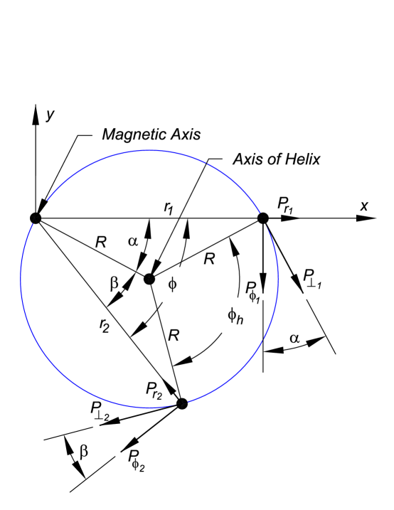
Figure 1: Geometry of the helical trajectory of a particle of total momentum $P$ that enters a solenoid magnet at $(r,\phi,z)=(r_{1}=d_{1}\theta_{1},0,0)$ with radial momentum $P_{r_{1}}=P\theta_{1}$. The fringe field at the entrance of the solenoid gives the particle an azimuthal kick resulting in momentum $P_{\phi_{1}}=-eBr_{1}/2c$, where the magnetic field is ${\bf B}=B\hat{\bf z}$ inside the solenoid. The helix has radius $R=cP_{\perp}/eB$. At the exit of the solenoid the particle is at $(r_{2},\phi,L)$ where $\phi=-eBL/2cP=\phi_{h}/2$; the azimuthal rotation of the particle’s trajectory about the magnetic axis is one half that about the axis of the helix.

The fringe field at the entrance of the solenoid gives the particle an azimuthal kick resulting in momentum

$$P_{\phi_{1}}=-{eBr_{1}\over 2c}=-{eBd_{1}\theta_{1}\over 2c}\,,$$ (30)

according to eq. (25), where the magnetic field is ${\bf B}=B\hat{\bf z}$ inside the solenoid. The transverse momentum $P_{\perp}$ of the particle inside the magnet is therefore

$$P_{\perp}=\sqrt{P^{2}_{r_{1}}+P^{2}_{\phi_{1}}}={eBr_{1}\over 2c}\sqrt{1+\left({2cP\over eBd_{1}}\right)^{2}}={eBr_{1}\over 2c}\sqrt{1+\left({2{\mathchoice{\hbox{\raise 5.06941pt\hbox to0.0pt{\kern 1.45833pt\vrule width=2.91667pt,height=0.1pt,depth=0.1pt\hss}\hbox{$\displaystyle\lambda$}}}{\hbox{\raise 5.06941pt\hbox to0.0pt{\kern 1.45833pt\vrule width=2.91667pt,height=0.1pt,depth=0.1pt\hss}\hbox{$\textstyle\lambda$}}}{\hbox{\raise 3.54857pt\hbox to0.0pt{\kern 1.02083pt\vrule width=2.04167pt,height=0.1pt,depth=0.1pt\hss}\hbox{$\scriptstyle\lambda$}}}{\hbox{\raise 2.5347pt\hbox to0.0pt{\kern 0.72916pt\vrule width=1.45833pt,height=0.1pt,depth=0.1pt\hss}\hbox{$\scriptscriptstyle\lambda$}}}}\over d_{1}}\right)^{2}}={eBR\over c}\,,$$ (31)

where $R$ is the radius of the helical trajectory of the particle inside the solenoid, recalling eq. (15). We also can write

$$r_{1}=2R\cos\alpha,$$ (32)

where the angle $\alpha$, shown in Fig. 1, is related by

$$\tan\alpha={P_{r_{1}}\over\left|P_{\phi_{1}}\right|}={2cP\over eBd_{1}}={2{\mathchoice{\hbox{\raise 5.06941pt\hbox to0.0pt{\kern 1.45833pt\vrule width=2.91667pt,height=0.1pt,depth=0.1pt\hss}\hbox{$\displaystyle\lambda$}}}{\hbox{\raise 5.06941pt\hbox to0.0pt{\kern 1.45833pt\vrule width=2.91667pt,height=0.1pt,depth=0.1pt\hss}\hbox{$\textstyle\lambda$}}}{\hbox{\raise 3.54857pt\hbox to0.0pt{\kern 1.02083pt\vrule width=2.04167pt,height=0.1pt,depth=0.1pt\hss}\hbox{$\scriptstyle\lambda$}}}{\hbox{\raise 2.5347pt\hbox to0.0pt{\kern 0.72916pt\vrule width=1.45833pt,height=0.1pt,depth=0.1pt\hss}\hbox{$\scriptscriptstyle\lambda$}}}}\over d_{1}}\,,$$ (33)

which is independent of the production angle $\theta_{1}$ in the paraxial approximation.

As the particle traverses length $L$ of the solenoid, its trajectory rotates by azimuthal angle

$$\phi_{h}=-{eBL\over cP}=-{L\over{\mathchoice{\hbox{\raise 5.06941pt\hbox to0.0pt{\kern 1.45833pt\vrule width=2.91667pt,height=0.1pt,depth=0.1pt\hss}\hbox{$\displaystyle\lambda$}}}{\hbox{\raise 5.06941pt\hbox to0.0pt{\kern 1.45833pt\vrule width=2.91667pt,height=0.1pt,depth=0.1pt\hss}\hbox{$\textstyle\lambda$}}}{\hbox{\raise 3.54857pt\hbox to0.0pt{\kern 1.02083pt\vrule width=2.04167pt,height=0.1pt,depth=0.1pt\hss}\hbox{$\scriptstyle\lambda$}}}{\hbox{\raise 2.5347pt\hbox to0.0pt{\kern 0.72916pt\vrule width=1.45833pt,height=0.1pt,depth=0.1pt\hss}\hbox{$\scriptscriptstyle\lambda$}}}}}$$ (34)

about the axis of the helix. At the exit of the solenoid the particle is at $(r_{2},\phi,L)$ in cylindrical coordinates centered on the axis of the magnet (rather than on the axis of the helix), as shown in Fig. 1. By the well-known geometrical relation that the angle subtended by an arc on a circle as viewed from another point on that circle is one half the angle subtended by that arc from the center of the circle, we have that

$$\phi={\phi_{h}\over 2}=-{eBL\over 2cP}=-{L\over 2{\mathchoice{\hbox{\raise 5.06941pt\hbox to0.0pt{\kern 1.45833pt\vrule width=2.91667pt,height=0.1pt,depth=0.1pt\hss}\hbox{$\displaystyle\lambda$}}}{\hbox{\raise 5.06941pt\hbox to0.0pt{\kern 1.45833pt\vrule width=2.91667pt,height=0.1pt,depth=0.1pt\hss}\hbox{$\textstyle\lambda$}}}{\hbox{\raise 3.54857pt\hbox to0.0pt{\kern 1.02083pt\vrule width=2.04167pt,height=0.1pt,depth=0.1pt\hss}\hbox{$\scriptstyle\lambda$}}}{\hbox{\raise 2.5347pt\hbox to0.0pt{\kern 0.72916pt\vrule width=1.45833pt,height=0.1pt,depth=0.1pt\hss}\hbox{$\scriptscriptstyle\lambda$}}}}}\,.$$ (35)

The radial coordinate of the particle at the exit of the solenoid is

$$r_{2}=2R\cos\beta,$$ (36)

where angle $\beta$ is given by

$$\beta=\left|\phi\right|-\alpha={L\over 2{\mathchoice{\hbox{\raise 5.06941pt\hbox to0.0pt{\kern 1.45833pt\vrule width=2.91667pt,height=0.1pt,depth=0.1pt\hss}\hbox{$\displaystyle\lambda$}}}{\hbox{\raise 5.06941pt\hbox to0.0pt{\kern 1.45833pt\vrule width=2.91667pt,height=0.1pt,depth=0.1pt\hss}\hbox{$\textstyle\lambda$}}}{\hbox{\raise 3.54857pt\hbox to0.0pt{\kern 1.02083pt\vrule width=2.04167pt,height=0.1pt,depth=0.1pt\hss}\hbox{$\scriptstyle\lambda$}}}{\hbox{\raise 2.5347pt\hbox to0.0pt{\kern 0.72916pt\vrule width=1.45833pt,height=0.1pt,depth=0.1pt\hss}\hbox{$\scriptscriptstyle\lambda$}}}}}-\tan^{-1}\left({2{\mathchoice{\hbox{\raise 5.06941pt\hbox to0.0pt{\kern 1.45833pt\vrule width=2.91667pt,height=0.1pt,depth=0.1pt\hss}\hbox{$\displaystyle\lambda$}}}{\hbox{\raise 5.06941pt\hbox to0.0pt{\kern 1.45833pt\vrule width=2.91667pt,height=0.1pt,depth=0.1pt\hss}\hbox{$\textstyle\lambda$}}}{\hbox{\raise 3.54857pt\hbox to0.0pt{\kern 1.02083pt\vrule width=2.04167pt,height=0.1pt,depth=0.1pt\hss}\hbox{$\scriptstyle\lambda$}}}{\hbox{\raise 2.5347pt\hbox to0.0pt{\kern 0.72916pt\vrule width=1.45833pt,height=0.1pt,depth=0.1pt\hss}\hbox{$\scriptscriptstyle\lambda$}}}}\over d_{1}}\right).$$ (37)

When the particle is at the exit of the solenoid, but still inside it, the transverse momentum vector ${\bf P}_{\perp_{2}}$ makes angle $\beta$ to the unit vector $\hat{\phi}$, as shown in Fig. 1. The radial momentum of the particle $P_{r_{2}}$ at the exit of the magnet is therefore

$$P_{r_{2}}=-P_{\perp}\sin\beta=-P_{\perp}{r_{2}\over 2R}\tan\beta=-{eBr_{2}\over 2c}{\tan{L\over 2{\mathchoice{\hbox{\raise 5.06941pt\hbox to0.0pt{\kern 1.45833pt\vrule width=2.91667pt,height=0.1pt,depth=0.1pt\hss}\hbox{$\displaystyle\lambda$}}}{\hbox{\raise 5.06941pt\hbox to0.0pt{\kern 1.45833pt\vrule width=2.91667pt,height=0.1pt,depth=0.1pt\hss}\hbox{$\textstyle\lambda$}}}{\hbox{\raise 3.54857pt\hbox to0.0pt{\kern 1.02083pt\vrule width=2.04167pt,height=0.1pt,depth=0.1pt\hss}\hbox{$\scriptstyle\lambda$}}}{\hbox{\raise 2.5347pt\hbox to0.0pt{\kern 0.72916pt\vrule width=1.45833pt,height=0.1pt,depth=0.1pt\hss}\hbox{$\scriptscriptstyle\lambda$}}}}}-{2{\mathchoice{\hbox{\raise 5.06941pt\hbox to0.0pt{\kern 1.45833pt\vrule width=2.91667pt,height=0.1pt,depth=0.1pt\hss}\hbox{$\displaystyle\lambda$}}}{\hbox{\raise 5.06941pt\hbox to0.0pt{\kern 1.45833pt\vrule width=2.91667pt,height=0.1pt,depth=0.1pt\hss}\hbox{$\textstyle\lambda$}}}{\hbox{\raise 3.54857pt\hbox to0.0pt{\kern 1.02083pt\vrule width=2.04167pt,height=0.1pt,depth=0.1pt\hss}\hbox{$\scriptstyle\lambda$}}}{\hbox{\raise 2.5347pt\hbox to0.0pt{\kern 0.72916pt\vrule width=1.45833pt,height=0.1pt,depth=0.1pt\hss}\hbox{$\scriptscriptstyle\lambda$}}}}\over d_{1}}\over 1+{2{\mathchoice{\hbox{\raise 5.06941pt\hbox to0.0pt{\kern 1.45833pt\vrule width=2.91667pt,height=0.1pt,depth=0.1pt\hss}\hbox{$\displaystyle\lambda$}}}{\hbox{\raise 5.06941pt\hbox to0.0pt{\kern 1.45833pt\vrule width=2.91667pt,height=0.1pt,depth=0.1pt\hss}\hbox{$\textstyle\lambda$}}}{\hbox{\raise 3.54857pt\hbox to0.0pt{\kern 1.02083pt\vrule width=2.04167pt,height=0.1pt,depth=0.1pt\hss}\hbox{$\scriptstyle\lambda$}}}{\hbox{\raise 2.5347pt\hbox to0.0pt{\kern 0.72916pt\vrule width=1.45833pt,height=0.1pt,depth=0.1pt\hss}\hbox{$\scriptscriptstyle\lambda$}}}}\over d_{1}}\tan{L\over 2{\mathchoice{\hbox{\raise 3.54857pt\hbox to0.0pt{\kern 1.02083pt\vrule width=2.04167pt,height=0.1pt,depth=0.1pt\hss}\hbox{$\displaystyle\lambda$}}}{\hbox{\raise 3.54857pt\hbox to0.0pt{\kern 1.02083pt\vrule width=2.04167pt,height=0.1pt,depth=0.1pt\hss}\hbox{$\textstyle\lambda$}}}{\hbox{\raise 2.484pt\hbox to0.0pt{\kern 0.71458pt\vrule width=1.42917pt,height=0.1pt,depth=0.1pt\hss}\hbox{$\scriptstyle\lambda$}}}{\hbox{\raise 1.77428pt\hbox to0.0pt{\kern 0.5104pt\vrule width=1.02083pt,height=0.1pt,depth=0.1pt\hss}\hbox{$\scriptscriptstyle\lambda$}}}}}}\,,$$ (38)

using eqs. (31) and (36), while the azimuthal component $P_{\phi_{2}}$ obeys

$$P_{\phi_{2}}=-P_{\perp}\cos\beta=-{eBr_{2}\over 2c}\,.$$ (39)

As the particle exits the magnet, the radial component of its transverse momentum remains at the value of eq. (38) in the impulse approximation, while the azimuthal component increases by $eBr_{2}/2c$ over the value of eq. (39) and hence vanishes, as expected since the canonical angular momentum is zero.

Once the particle has exited the magnet its transverse momentum is purely radial, with a value proportional to the radial coordinate $r_{2}$ at the exit of the magnet. This is lens-like behavior, in that the particle will then cross the magnetic axis at distance $d_{2}$ from the exit of the magnet, where

$${r_{2}\over d_{2}}=\theta_{2}={P_{r_{2}}\over P}\,.$$ (40)

and so

$$d_{2}={2cP\over eB\tan\beta}=2{\mathchoice{\hbox{\raise 5.06941pt\hbox to0.0pt{\kern 1.45833pt\vrule width=2.91667pt,height=0.1pt,depth=0.1pt\hss}\hbox{$\displaystyle\lambda$}}}{\hbox{\raise 5.06941pt\hbox to0.0pt{\kern 1.45833pt\vrule width=2.91667pt,height=0.1pt,depth=0.1pt\hss}\hbox{$\textstyle\lambda$}}}{\hbox{\raise 3.54857pt\hbox to0.0pt{\kern 1.02083pt\vrule width=2.04167pt,height=0.1pt,depth=0.1pt\hss}\hbox{$\scriptstyle\lambda$}}}{\hbox{\raise 2.5347pt\hbox to0.0pt{\kern 0.72916pt\vrule width=1.45833pt,height=0.1pt,depth=0.1pt\hss}\hbox{$\scriptscriptstyle\lambda$}}}}{1+{2{\mathchoice{\hbox{\raise 5.06941pt\hbox to0.0pt{\kern 1.45833pt\vrule width=2.91667pt,height=0.1pt,depth=0.1pt\hss}\hbox{$\displaystyle\lambda$}}}{\hbox{\raise 5.06941pt\hbox to0.0pt{\kern 1.45833pt\vrule width=2.91667pt,height=0.1pt,depth=0.1pt\hss}\hbox{$\textstyle\lambda$}}}{\hbox{\raise 3.54857pt\hbox to0.0pt{\kern 1.02083pt\vrule width=2.04167pt,height=0.1pt,depth=0.1pt\hss}\hbox{$\scriptstyle\lambda$}}}{\hbox{\raise 2.5347pt\hbox to0.0pt{\kern 0.72916pt\vrule width=1.45833pt,height=0.1pt,depth=0.1pt\hss}\hbox{$\scriptscriptstyle\lambda$}}}}\over d_{1}}\tan{L\over 2{\mathchoice{\hbox{\raise 5.06941pt\hbox to0.0pt{\kern 1.45833pt\vrule width=2.91667pt,height=0.1pt,depth=0.1pt\hss}\hbox{$\displaystyle\lambda$}}}{\hbox{\raise 5.06941pt\hbox to0.0pt{\kern 1.45833pt\vrule width=2.91667pt,height=0.1pt,depth=0.1pt\hss}\hbox{$\textstyle\lambda$}}}{\hbox{\raise 3.54857pt\hbox to0.0pt{\kern 1.02083pt\vrule width=2.04167pt,height=0.1pt,depth=0.1pt\hss}\hbox{$\scriptstyle\lambda$}}}{\hbox{\raise 2.5347pt\hbox to0.0pt{\kern 0.72916pt\vrule width=1.45833pt,height=0.1pt,depth=0.1pt\hss}\hbox{$\scriptscriptstyle\lambda$}}}}}\over\tan{L\over 2{\mathchoice{\hbox{\raise 3.54857pt\hbox to0.0pt{\kern 1.02083pt\vrule width=2.04167pt,height=0.1pt,depth=0.1pt\hss}\hbox{$\displaystyle\lambda$}}}{\hbox{\raise 3.54857pt\hbox to0.0pt{\kern 1.02083pt\vrule width=2.04167pt,height=0.1pt,depth=0.1pt\hss}\hbox{$\textstyle\lambda$}}}{\hbox{\raise 2.484pt\hbox to0.0pt{\kern 0.71458pt\vrule width=1.42917pt,height=0.1pt,depth=0.1pt\hss}\hbox{$\scriptstyle\lambda$}}}{\hbox{\raise 1.77428pt\hbox to0.0pt{\kern 0.5104pt\vrule width=1.02083pt,height=0.1pt,depth=0.1pt\hss}\hbox{$\scriptscriptstyle\lambda$}}}}}-{2{\mathchoice{\hbox{\raise 5.06941pt\hbox to0.0pt{\kern 1.45833pt\vrule width=2.91667pt,height=0.1pt,depth=0.1pt\hss}\hbox{$\displaystyle\lambda$}}}{\hbox{\raise 5.06941pt\hbox to0.0pt{\kern 1.45833pt\vrule width=2.91667pt,height=0.1pt,depth=0.1pt\hss}\hbox{$\textstyle\lambda$}}}{\hbox{\raise 3.54857pt\hbox to0.0pt{\kern 1.02083pt\vrule width=2.04167pt,height=0.1pt,depth=0.1pt\hss}\hbox{$\scriptstyle\lambda$}}}{\hbox{\raise 2.5347pt\hbox to0.0pt{\kern 0.72916pt\vrule width=1.45833pt,height=0.1pt,depth=0.1pt\hss}\hbox{$\scriptscriptstyle\lambda$}}}}\over d_{1}}}={fd_{1}\over d_{1}-f}\left(1+{2{\mathchoice{\hbox{\raise 5.06941pt\hbox to0.0pt{\kern 1.45833pt\vrule width=2.91667pt,height=0.1pt,depth=0.1pt\hss}\hbox{$\displaystyle\lambda$}}}{\hbox{\raise 5.06941pt\hbox to0.0pt{\kern 1.45833pt\vrule width=2.91667pt,height=0.1pt,depth=0.1pt\hss}\hbox{$\textstyle\lambda$}}}{\hbox{\raise 3.54857pt\hbox to0.0pt{\kern 1.02083pt\vrule width=2.04167pt,height=0.1pt,depth=0.1pt\hss}\hbox{$\scriptstyle\lambda$}}}{\hbox{\raise 2.5347pt\hbox to0.0pt{\kern 0.72916pt\vrule width=1.45833pt,height=0.1pt,depth=0.1pt\hss}\hbox{$\scriptscriptstyle\lambda$}}}}\over d_{1}}\tan{L\over 2{\mathchoice{\hbox{\raise 5.06941pt\hbox to0.0pt{\kern 1.45833pt\vrule width=2.91667pt,height=0.1pt,depth=0.1pt\hss}\hbox{$\displaystyle\lambda$}}}{\hbox{\raise 5.06941pt\hbox to0.0pt{\kern 1.45833pt\vrule width=2.91667pt,height=0.1pt,depth=0.1pt\hss}\hbox{$\textstyle\lambda$}}}{\hbox{\raise 3.54857pt\hbox to0.0pt{\kern 1.02083pt\vrule width=2.04167pt,height=0.1pt,depth=0.1pt\hss}\hbox{$\scriptstyle\lambda$}}}{\hbox{\raise 2.5347pt\hbox to0.0pt{\kern 0.72916pt\vrule width=1.45833pt,height=0.1pt,depth=0.1pt\hss}\hbox{$\scriptscriptstyle\lambda$}}}}}\right)\,,$$ (41)

where

$$f={2{\mathchoice{\hbox{\raise 5.06941pt\hbox to0.0pt{\kern 1.45833pt\vrule width=2.91667pt,height=0.1pt,depth=0.1pt\hss}\hbox{$\displaystyle\lambda$}}}{\hbox{\raise 5.06941pt\hbox to0.0pt{\kern 1.45833pt\vrule width=2.91667pt,height=0.1pt,depth=0.1pt\hss}\hbox{$\textstyle\lambda$}}}{\hbox{\raise 3.54857pt\hbox to0.0pt{\kern 1.02083pt\vrule width=2.04167pt,height=0.1pt,depth=0.1pt\hss}\hbox{$\scriptstyle\lambda$}}}{\hbox{\raise 2.5347pt\hbox to0.0pt{\kern 0.72916pt\vrule width=1.45833pt,height=0.1pt,depth=0.1pt\hss}\hbox{$\scriptscriptstyle\lambda$}}}}\over\tan{L\over 2{\mathchoice{\hbox{\raise 3.54857pt\hbox to0.0pt{\kern 1.02083pt\vrule width=2.04167pt,height=0.1pt,depth=0.1pt\hss}\hbox{$\displaystyle\lambda$}}}{\hbox{\raise 3.54857pt\hbox to0.0pt{\kern 1.02083pt\vrule width=2.04167pt,height=0.1pt,depth=0.1pt\hss}\hbox{$\textstyle\lambda$}}}{\hbox{\raise 2.484pt\hbox to0.0pt{\kern 0.71458pt\vrule width=1.42917pt,height=0.1pt,depth=0.1pt\hss}\hbox{$\scriptstyle\lambda$}}}{\hbox{\raise 1.77428pt\hbox to0.0pt{\kern 0.5104pt\vrule width=1.02083pt,height=0.1pt,depth=0.1pt\hss}\hbox{$\scriptscriptstyle\lambda$}}}}}}\,.$$ (42)

When distance $d_{2}$ is positive the solenoid acts as a (thick) focusing lens.

For the special cases of point-to-parallel focusing ($d_{2}\to\infty$) and parallel-to-point focusing ($d_{1}\to\infty$), the solenoid magnet has focal length $f$ given by eq. (42).

If $(2{\mathchoice{\hbox{\raise 5.06941pt\hbox to0.0pt{\kern 1.45833pt\vrule width=2.91667pt,height=0.1pt,depth=0.1pt\hss}\hbox{$\displaystyle\lambda$}}}{\hbox{\raise 5.06941pt\hbox to0.0pt{\kern 1.45833pt\vrule width=2.91667pt,height=0.1pt,depth=0.1pt\hss}\hbox{$\textstyle\lambda$}}}{\hbox{\raise 3.54857pt\hbox to0.0pt{\kern 1.02083pt\vrule width=2.04167pt,height=0.1pt,depth=0.1pt\hss}\hbox{$\scriptstyle\lambda$}}}{\hbox{\raise 2.5347pt\hbox to0.0pt{\kern 0.72916pt\vrule width=1.45833pt,height=0.1pt,depth=0.1pt\hss}\hbox{$\scriptscriptstyle\lambda$}}}}/d_{1})\tan(L/2{\mathchoice{\hbox{\raise 5.06941pt\hbox to0.0pt{\kern 1.45833pt\vrule width=2.91667pt,height=0.1pt,depth=0.1pt\hss}\hbox{$\displaystyle\lambda$}}}{\hbox{\raise 5.06941pt\hbox to0.0pt{\kern 1.45833pt\vrule width=2.91667pt,height=0.1pt,depth=0.1pt\hss}\hbox{$\textstyle\lambda$}}}{\hbox{\raise 3.54857pt\hbox to0.0pt{\kern 1.02083pt\vrule width=2.04167pt,height=0.1pt,depth=0.1pt\hss}\hbox{$\scriptstyle\lambda$}}}{\hbox{\raise 2.5347pt\hbox to0.0pt{\kern 0.72916pt\vrule width=1.45833pt,height=0.1pt,depth=0.1pt\hss}\hbox{$\scriptscriptstyle\lambda$}}}})\ll 1$ then the object distance $d_{1}$ and the image distance $d_{2}$ obey the lens formula

$${1\over d_{1}}+{1\over d_{2}}={1\over f}\qquad\left(\tan{L\over 2{\mathchoice{\hbox{\raise 5.06941pt\hbox to0.0pt{\kern 1.45833pt\vrule width=2.91667pt,height=0.1pt,depth=0.1pt\hss}\hbox{$\displaystyle\lambda$}}}{\hbox{\raise 5.06941pt\hbox to0.0pt{\kern 1.45833pt\vrule width=2.91667pt,height=0.1pt,depth=0.1pt\hss}\hbox{$\textstyle\lambda$}}}{\hbox{\raise 3.54857pt\hbox to0.0pt{\kern 1.02083pt\vrule width=2.04167pt,height=0.1pt,depth=0.1pt\hss}\hbox{$\scriptstyle\lambda$}}}{\hbox{\raise 2.5347pt\hbox to0.0pt{\kern 0.72916pt\vrule width=1.45833pt,height=0.1pt,depth=0.1pt\hss}\hbox{$\scriptscriptstyle\lambda$}}}}}\ll{d_{1}\over 2{\mathchoice{\hbox{\raise 5.06941pt\hbox to0.0pt{\kern 1.45833pt\vrule width=2.91667pt,height=0.1pt,depth=0.1pt\hss}\hbox{$\displaystyle\lambda$}}}{\hbox{\raise 5.06941pt\hbox to0.0pt{\kern 1.45833pt\vrule width=2.91667pt,height=0.1pt,depth=0.1pt\hss}\hbox{$\textstyle\lambda$}}}{\hbox{\raise 3.54857pt\hbox to0.0pt{\kern 1.02083pt\vrule width=2.04167pt,height=0.1pt,depth=0.1pt\hss}\hbox{$\scriptstyle\lambda$}}}{\hbox{\raise 2.5347pt\hbox to0.0pt{\kern 0.72916pt\vrule width=1.45833pt,height=0.1pt,depth=0.1pt\hss}\hbox{$\scriptscriptstyle\lambda$}}}}}\right).$$ (43)

If in addition the length $L$ of the solenoid is small compared to the Larmor wavelength  $\textstyle\lambda$ the solenoid can be called a thin lens, for which

$$f={4{\mathchoice{\hbox{\raise 5.06941pt\hbox to0.0pt{\kern 1.45833pt\vrule width=2.91667pt,height=0.1pt,depth=0.1pt\hss}\hbox{$\displaystyle\lambda$}}}{\hbox{\raise 5.06941pt\hbox to0.0pt{\kern 1.45833pt\vrule width=2.91667pt,height=0.1pt,depth=0.1pt\hss}\hbox{$\textstyle\lambda$}}}{\hbox{\raise 3.54857pt\hbox to0.0pt{\kern 1.02083pt\vrule width=2.04167pt,height=0.1pt,depth=0.1pt\hss}\hbox{$\scriptstyle\lambda$}}}{\hbox{\raise 2.5347pt\hbox to0.0pt{\kern 0.72916pt\vrule width=1.45833pt,height=0.1pt,depth=0.1pt\hss}\hbox{$\scriptscriptstyle\lambda$}}}}^{2}\over L}\qquad(\mbox{thin\ lens}:L\ll{\mathchoice{\hbox{\raise 5.06941pt\hbox to0.0pt{\kern 1.45833pt\vrule width=2.91667pt,height=0.1pt,depth=0.1pt\hss}\hbox{$\displaystyle\lambda$}}}{\hbox{\raise 5.06941pt\hbox to0.0pt{\kern 1.45833pt\vrule width=2.91667pt,height=0.1pt,depth=0.1pt\hss}\hbox{$\textstyle\lambda$}}}{\hbox{\raise 3.54857pt\hbox to0.0pt{\kern 1.02083pt\vrule width=2.04167pt,height=0.1pt,depth=0.1pt\hss}\hbox{$\scriptstyle\lambda$}}}{\hbox{\raise 2.5347pt\hbox to0.0pt{\kern 0.72916pt\vrule width=1.45833pt,height=0.1pt,depth=0.1pt\hss}\hbox{$\scriptscriptstyle\lambda$}}}},\ L\ll d_{1}).$$ (44)

This weakly focusing limit is, however, seldom achieved in practical applications of solenoid magnets as focusing elements.

The results (41)-(44) for thick- and thin-lens focusing can be utilized in a transfer-matrix description of particle transport through magnetic systems [5].

2.5 Particle Source Inside the Magnet

The case of a source of particles inside the solenoid magnet, say at $z=0$, can be treated as a special case of the analysis in sec. 2.4 in which $d_{1}=r_{1}=0$. The angle $\alpha$ shown in Fig. 1 is $\pi/2$ in this case, so that angle $\beta$ is

$$\beta={L\over 2{\mathchoice{\hbox{\raise 5.06941pt\hbox to0.0pt{\kern 1.45833pt\vrule width=2.91667pt,height=0.1pt,depth=0.1pt\hss}\hbox{$\displaystyle\lambda$}}}{\hbox{\raise 5.06941pt\hbox to0.0pt{\kern 1.45833pt\vrule width=2.91667pt,height=0.1pt,depth=0.1pt\hss}\hbox{$\textstyle\lambda$}}}{\hbox{\raise 3.54857pt\hbox to0.0pt{\kern 1.02083pt\vrule width=2.04167pt,height=0.1pt,depth=0.1pt\hss}\hbox{$\scriptstyle\lambda$}}}{\hbox{\raise 2.5347pt\hbox to0.0pt{\kern 0.72916pt\vrule width=1.45833pt,height=0.1pt,depth=0.1pt\hss}\hbox{$\scriptscriptstyle\lambda$}}}}}-{\pi\over 2}\,.$$ (45)

The radial coordinate of the particle at the exit of the magnet is

$$r_{2}=2R\cos\beta=2R\sin{L\over 2{\mathchoice{\hbox{\raise 5.06941pt\hbox to0.0pt{\kern 1.45833pt\vrule width=2.91667pt,height=0.1pt,depth=0.1pt\hss}\hbox{$\displaystyle\lambda$}}}{\hbox{\raise 5.06941pt\hbox to0.0pt{\kern 1.45833pt\vrule width=2.91667pt,height=0.1pt,depth=0.1pt\hss}\hbox{$\textstyle\lambda$}}}{\hbox{\raise 3.54857pt\hbox to0.0pt{\kern 1.02083pt\vrule width=2.04167pt,height=0.1pt,depth=0.1pt\hss}\hbox{$\scriptstyle\lambda$}}}{\hbox{\raise 2.5347pt\hbox to0.0pt{\kern 0.72916pt\vrule width=1.45833pt,height=0.1pt,depth=0.1pt\hss}\hbox{$\scriptscriptstyle\lambda$}}}}}\,,$$ (46)

and the image distance $d_{2}$ follows from eq. (41) as

$$d_{2}={2cP\over eB\tan\beta}=-2{\mathchoice{\hbox{\raise 5.06941pt\hbox to0.0pt{\kern 1.45833pt\vrule width=2.91667pt,height=0.1pt,depth=0.1pt\hss}\hbox{$\displaystyle\lambda$}}}{\hbox{\raise 5.06941pt\hbox to0.0pt{\kern 1.45833pt\vrule width=2.91667pt,height=0.1pt,depth=0.1pt\hss}\hbox{$\textstyle\lambda$}}}{\hbox{\raise 3.54857pt\hbox to0.0pt{\kern 1.02083pt\vrule width=2.04167pt,height=0.1pt,depth=0.1pt\hss}\hbox{$\scriptstyle\lambda$}}}{\hbox{\raise 2.5347pt\hbox to0.0pt{\kern 0.72916pt\vrule width=1.45833pt,height=0.1pt,depth=0.1pt\hss}\hbox{$\scriptscriptstyle\lambda$}}}}\tan{L\over 2{\mathchoice{\hbox{\raise 5.06941pt\hbox to0.0pt{\kern 1.45833pt\vrule width=2.91667pt,height=0.1pt,depth=0.1pt\hss}\hbox{$\displaystyle\lambda$}}}{\hbox{\raise 5.06941pt\hbox to0.0pt{\kern 1.45833pt\vrule width=2.91667pt,height=0.1pt,depth=0.1pt\hss}\hbox{$\textstyle\lambda$}}}{\hbox{\raise 3.54857pt\hbox to0.0pt{\kern 1.02083pt\vrule width=2.04167pt,height=0.1pt,depth=0.1pt\hss}\hbox{$\scriptstyle\lambda$}}}{\hbox{\raise 2.5347pt\hbox to0.0pt{\kern 0.72916pt\vrule width=1.45833pt,height=0.1pt,depth=0.1pt\hss}\hbox{$\scriptscriptstyle\lambda$}}}}}\,.$$ (47)

The radial momentum at the exit of the magnet is

$$P_{r_{2}}=-P_{\perp}\sin\beta=-{eBR\over c}{r_{2}\over 2R}\tan\beta={eBr_{2}\over 2c}\cot{L\over 2{\mathchoice{\hbox{\raise 5.06941pt\hbox to0.0pt{\kern 1.45833pt\vrule width=2.91667pt,height=0.1pt,depth=0.1pt\hss}\hbox{$\displaystyle\lambda$}}}{\hbox{\raise 5.06941pt\hbox to0.0pt{\kern 1.45833pt\vrule width=2.91667pt,height=0.1pt,depth=0.1pt\hss}\hbox{$\textstyle\lambda$}}}{\hbox{\raise 3.54857pt\hbox to0.0pt{\kern 1.02083pt\vrule width=2.04167pt,height=0.1pt,depth=0.1pt\hss}\hbox{$\scriptstyle\lambda$}}}{\hbox{\raise 2.5347pt\hbox to0.0pt{\kern 0.72916pt\vrule width=1.45833pt,height=0.1pt,depth=0.1pt\hss}\hbox{$\scriptscriptstyle\lambda$}}}}}\,.$$ (48)

according to eqs. (38) and (45).

This is lens-like behavior ($P_{r_{2}}\propto r_{2}$) for any length $L$ of the solenoid, with $L=n\pi{\mathchoice{\hbox{\raise 5.06941pt\hbox to0.0pt{\kern 1.45833pt\vrule width=2.91667pt,height=0.1pt,depth=0.1pt\hss}\hbox{$\displaystyle\lambda$}}}{\hbox{\raise 5.06941pt\hbox to0.0pt{\kern 1.45833pt\vrule width=2.91667pt,height=0.1pt,depth=0.1pt\hss}\hbox{$\textstyle\lambda$}}}{\hbox{\raise 3.54857pt\hbox to0.0pt{\kern 1.02083pt\vrule width=2.04167pt,height=0.1pt,depth=0.1pt\hss}\hbox{$\scriptstyle\lambda$}}}{\hbox{\raise 2.5347pt\hbox to0.0pt{\kern 0.72916pt\vrule width=1.45833pt,height=0.1pt,depth=0.1pt\hss}\hbox{$\scriptscriptstyle\lambda$}}}}$ being the boundary between focusing and defocusing.

For the special case that $L=2n\pi{\mathchoice{\hbox{\raise 5.06941pt\hbox to0.0pt{\kern 1.45833pt\vrule width=2.91667pt,height=0.1pt,depth=0.1pt\hss}\hbox{$\displaystyle\lambda$}}}{\hbox{\raise 5.06941pt\hbox to0.0pt{\kern 1.45833pt\vrule width=2.91667pt,height=0.1pt,depth=0.1pt\hss}\hbox{$\textstyle\lambda$}}}{\hbox{\raise 3.54857pt\hbox to0.0pt{\kern 1.02083pt\vrule width=2.04167pt,height=0.1pt,depth=0.1pt\hss}\hbox{$\scriptstyle\lambda$}}}{\hbox{\raise 2.5347pt\hbox to0.0pt{\kern 0.72916pt\vrule width=1.45833pt,height=0.1pt,depth=0.1pt\hss}\hbox{$\scriptscriptstyle\lambda$}}}}$ we have $d_{2}=r_{2}=0$, corresponding to an image of the source occuring at the exit of the magnet.

Of particular interest here is the special case that $L=(2n+1)\pi{\mathchoice{\hbox{\raise 5.06941pt\hbox to0.0pt{\kern 1.45833pt\vrule width=2.91667pt,height=0.1pt,depth=0.1pt\hss}\hbox{$\displaystyle\lambda$}}}{\hbox{\raise 5.06941pt\hbox to0.0pt{\kern 1.45833pt\vrule width=2.91667pt,height=0.1pt,depth=0.1pt\hss}\hbox{$\textstyle\lambda$}}}{\hbox{\raise 3.54857pt\hbox to0.0pt{\kern 1.02083pt\vrule width=2.04167pt,height=0.1pt,depth=0.1pt\hss}\hbox{$\scriptstyle\lambda$}}}{\hbox{\raise 2.5347pt\hbox to0.0pt{\kern 0.72916pt\vrule width=1.45833pt,height=0.1pt,depth=0.1pt\hss}\hbox{$\scriptscriptstyle\lambda$}}}}$, for which $d_{2}=\infty$, $P_{r_{2}}=0$, and we have point-to-parallel focusing. From Fig. 1 and eq. (48) we see that the condition for point-to-parallel focusing of a source inside the solenoid is that the particle has completed an odd number of half turns on its helical trajectory when it reaches the end of the solenoid. In this case we can say that the focal length of the solenoid lens is just the length $L$,

$$f=L=(2n+1)\pi{cP\over eB}\qquad\mbox{(point-to-parallel\ focus,\ source\ inside\ solenoid)}.$$ (49)

2.5.1 Neutrino Horn: Point-to-Parallel Focus, $L=(2n+1)\pi cP/eB$

A solenoid magnet provides point-to-parallel focusing for particles produced inside the magnet, on its axis, with a discrete set of momenta $P_{n}$ given by

$$P_{n}={P_{0}\over 2n+1}\,,\quad(n=0,1,2,....)\qquad\mbox{where}\qquad P_{0}={eBL\over\pi c}\,.$$ (50)

Particles with other momenta are not brought into parallelism, so that a “beam” formed by drifting particles that emerge from the solenoid will be quasimonochromatic with the sequence of momenta given in eq. (50). Figure 2 illustrates trajectories for particles of momenta $P_{0}$ and $3P_{0}$ in a solenoid magnet.

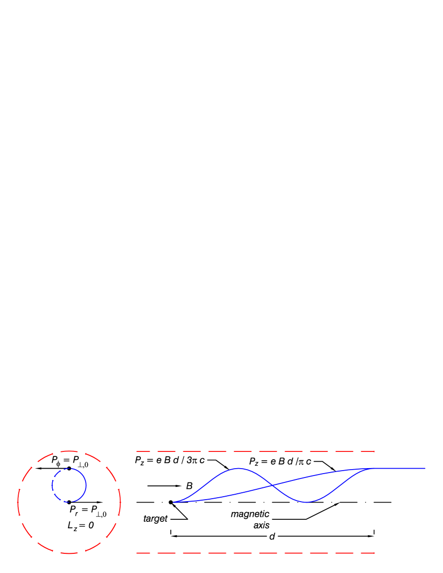
Figure 2: Concept of a neutrino horn based on solenoid focusing. The pion production target is inside the uniform field region of the solenoid. The focusing effects of the fringe field at the exit of the magnet (at distance $L$ from the target) act as ideal thin lens of focal length $L$ for a discrete set of particle momenta, given in eq. (50).

Such a sequence of momenta occurs in the phenomenon of neutrino oscillations over a flight path $l$. As is well, known, in the approximation of pure two-neutrino mixing, the probability that neutrino type (mass eigenstate) $i$ of energy $E=P$ appears are neutrino type $j$ after traversing distance $l$ is given by

$$\mbox{Prob}(i\to j)\propto\sin^{2}{\Delta M^{2}_{ij}l\over 2E}\,,$$ (51)

where $\Delta M_{ij}=M_{i}-M_{j}$ is the difference in the masses of the two neutrino types. Hence, for a fixed drift distance $l$, the probability of neutrino type $i$ appearing as type $j$ is maximal for the sequence of neutrino momenta (energy)

$$P_{n}={P_{0}\over 2n+1}\,,\quad(n=0,1,2,....)\qquad\mbox{where}\qquad P_{0}={\Delta M^{2}_{ij}l\over\pi}\,.$$ (52)

Thus a solenoid magnet could be very useful in preparing a neutrino beam with a sequence of momenta such that all oscillation effects are maximal. The potential advantage of such a beam for the study of CP violation in neutrino oscillations has been pointed out by Marciano [6], and elaborated upon in [7].

Of course, neutrinos are neutral, so that a solenoid magnet cannot directly affect their trajectories. Rather, the solenoid magnet would be used to focus $\pi^{\pm}$ particles that are produced in the interaction of a proton beam with a nuclear target that is placed on the axis inside the magnet. The length $l$ of the magnet should be short enough that most pions of interest exit the magnet before decaying into neutrinos, according to

$$\pi^{+}\to\mu^{+}\nu_{\mu},\qquad\pi^{-}\to\mu^{-}\bar{\nu}_{\mu}.$$ (53)

Because of the low “Q” value of this decay, the direction of the neutrinos is very close to that of the pions, provided that latter have energies greater than a few hundred MeV. The forward-going neutrinos carry about 4/9 of their parent pion momentum, so the solenoid system should be chosen with a momentum $P_{0,\pi}$ equal to 9/4 of the highest desired neutrino momentum at which the oscillation probability is maximal, i.e.,

$$P_{0,\pi}\approx{9\over 4}P_{0,\nu}.$$ (54)

As implied by eq. (53), the solenoid-focused beam would contain both muon neutrinos and muon antineutrinos, in roughly equal numbers. This has the advantage to studies could be made simultaneously with both neutrino and antineutrino beams. However, for the study of CP violation it would be necessary to identify whether each interactions was due to a neutrino or an antineutrino. This identification must be provided by the detector in which the neutrino interacts. If the neutrinos oscillate into electron neutrinos or antineutrinos before they interact in a the detector, the latter must distinguish showers of electrons from positrons. This difficult experimental challenge can likely only be met by a magnetized liquid argon detector [8, 9, 10].

When studying the oscillation of muon neutrinos into electron neutrinos, the presence of electron neutrinos in the beam constitutes the limiting background. Electron neutrinos are present in the beam due to the 3-body decay of the muons from pion decay:

$$\pi^{+}\to\mu^{+}\nu_{\mu},\quad\mu^{+}\to e^{+}\nu_{e}\bar{\nu}_{\mu},\qquad\qquad\pi^{-}\to\mu^{-}\bar{\nu}_{\mu},\quad\mu^{-}\to e^{-}\bar{\nu}_{e}\nu_{\mu}.$$ (55)

The background of electron neutrinos, compared to the flux of muon neutrinos at a particular energy, is suppressed when the beam contains only a narrow range of momenta of the parent pions. This occurs because the muon neutrinos from the pion decay then have typically higher momentum that the electron neutrinos from the related muon decay. Hence, the solenoid-focused neutrino beam, with its quasi line spectrum of energies will have lower electron neutrino content, at least for highest-energy neutrino “lines”, compared to a wide-band neutrino beam.

A final advantage of the solenoid-focused beam is that the magnetic elements are farther removed transversely from the pion production target, and so can be made more radiation resistant to intense proton fluxes than is the case for more conventional toroid-focused neutrino “horns”. Further, the relatively open geometry of the solenoid lens will permit use of liquid metal target, as needed if the proton beam has several megawatts of power [11].

The author thanks Ron Davidson for the demonstration that conservation of the canonical momentum $p_{\phi}$ follows from the Lorentz force law.

References

• [1] K.T.Β McDonald, Canonical Angular Momentum of a Solenoid Field (Nov.Β 13, 1998), http://puhep1.princeton.edu/$\tilde{\phantom{a}}$mcdonald/examples/canon.pdf
• [2] K.T.Β McDonald, An Off-Axis Neutrino Beam (Nov.Β 6, 2001), hep-ex/0111033
• [3] L.D.Β Landau and E.M.Β Lifshitz, The Classical Theory of Fields, 4th ed.Β (Pergamon Press, Oxford, 1975), sec.Β 16.
• [4] See, for example, K.-J.Β Kim and C.-X.Β Wang, Formulas for Transverse Ionization Cooling in Solenoidal Focusing Channels, Phys.Β Rev.Β Lett.Β 85, 760 (2000), http://www-mucool.fnal.gov/mcnotes/public/ps/muc0092/muc0092.ps.gz
• [5] See, for example, H.Β Weidemann, Particle Accelerator Physics II: Nonlinear and Higher-Order Beam Dynamics (Springer-Verlag, New York, 1994), sec.Β 3.3.
• [6] W.J.Β Marciano, Extra Long Baseline Neutrino Oscillations and CP Violation, BNL-HET-01/31 (Aug.Β 2001), hep-ph/0108181.
• [7] M.V.Β Diwan et al., Very Long Baseline Neutrino Oscillation Experiments for Precise Measurements of Mixing Parameters and CP Violating Effects, Phys.Β Rev.Β D 68, 012002 (2003), hep-ph/0303081
• [8] D.B.Β Cline et al., LANNDD – a massive liquid argon detector for proton decay, supernova and solar neutrino studies and a neutrino factory, Nucl.Β Instr.Β and Meth.Β A503, 136 (2003), astro-ph/0105442
• [9] A.Β Badertscher et al., Magnetized Liquid Argon Detector for Electron Charge Sign Discrimination, Letter of Intent to the CERN SPSSC (Jan. 3, 2002), http://www.hep.princeton.edu/$\tilde{\phantom{a}}$mcdonald/nufact/uL@CERN_LOI.pdf
• [10] M.V.Β Diwan et al., Proposal to Measure the Efficiency of Electron Charge Sign Determination up to 10 GeV in a Magnetized Liquid Argon Detector (BNL P-965, Apr.Β 7, 2002), http://www.hep.princeton.edu/$\tilde{\phantom{a}}$mcdonald/nufact/bnl_loi/argonprop.pdf
• [11] A.Β Hassenein et al., An R&D Program for Targetry and Capture at a Neutrino Factory and Muon Collider Source, Nucl.Β Instr. and Meth.Β A503, 70 (2003).