Multivariate Analysis from a Statistical Point of View

Abstract

Multivariate Analysis is an increasingly common tool in experimental high energy physics; however, many of the common approaches were borrowed from other fields. We clarify what the goal of a multivariate algorithm should be for the search for a new particle and compare different approaches. We also translate the Neyman-Pearson theory into the language of statistical learning theory.

I Introduction

Multivariate Analysis is an increasingly common tool in experimental high energy physics; however, most of the common approaches were borrowed from other fields. Each of these algorithms were developed for their own particular task, thus they look quite different at their core. It is not obvious that what these different algorithms do internally is optimal for the the tasks which they perform within high energy physics. It is also quite difficult to compare these different algorithms due to the differences in the formalisms that were used to derive and/or document them. In Section II we introduce a formalism for a Learning Machine, which is general enough to encompass all of the techniques used within high energy physics. In Sections III & IV we review the statistical statements relevant to new particle searches and translate them into the formalism of statistical learning theory. In the remainder of the note, we look at the main results of statistical learning theory and their relevance to some of the common algorithms used within high energy physics.

II Formalism

Formally a Learning Machine is a family of functions $\mathcal{F}$ with domain $I$ and range $O$ parametrized by $\alpha\in\Lambda$. The domain can usually be thought of as, or at least embedded in, $\mathbb{R}^{d}$ and we generically denote points in the domain as $x$. The points $x$ can be referred to in many ways (e.g. patterns, events, inputs, examples, …). The range is most commonly $\mathbb{R}$, $[0,1]$, or just $\{0,1\}$. Elements of the range are denoted by $y$ and can be referred to in many ways (e.g. classes, target values, outputs, …). The parameters $\alpha$ specify a particular function $f_{\alpha}\in\mathcal{F}$ and the structure of $\alpha\in\Lambda$ depends upon the learning machine Vapnik:1968 ; Vapnik:2000 .

In the modern theory of machine learning, the performance of a learning machine is usually cast in the more pessimistic setting of risk. In general, the risk, $R$, of a learning machine is written as

$$R(\alpha)=\int Q(x,y;\alpha)~{}p(x,y)dxdy$$ (1)

where $Q$ measures some notion of loss between $f_{\alpha}(x)$ and the target value $y$. For example, when classifying events, the risk of mis-classification is given by Eq. 1 with $Q(x,y;\alpha)=|y-f_{\alpha}(x)|$. Similarly, for regression tasks one takes $Q(x,y;\alpha)=(y-f_{\alpha}(x))^{2}$. Most of the classic applications of learning machines can be cast into this formalism; however, searches for new particles place some strain on the notion of risk.

III Searches for New Particles

The conclusion of an experimental search for a new particle is a statistical statement – usually a declaration of discovery or a limit on the mass of the hypothetical particle. Thus, the appropriate notion of performance for a multivariate algorithm used in a search for a new particle is that performance measure which will maximize the chance of declaring a discovery or provide the tightest limits on the hypothetical particle. In principle, it should be a fairly straight-forward procedure to use the formal statistical statements to derive the most appropriate performance measure. This procedure is complicated by the fact that experimentalists (and statisticians) cannot settle on a formalism to use (i.e. Bayesians vs. Frequentists). As an example, let us consider the Frequentist theory developed by Neyman and Pearson Kendall . This was the basis for the results of the search for the Standard Model Higgs boson at LEP FinalLHWG:2003sz .

The Neyman-Pearson theory (which we review briefly for completeness) begins with two Hypotheses: the null hypothesis $H_{0}$ and the alternate hypothesis $H_{1}$ Kendall . In the case of a new particle search $H_{0}$ is identified with the currently accepted theory (i.e. the Standard Model) and is usually referred to as the “background-only” hypothesis. Similarly, $H_{1}$ is identified with the theory being tested usually referred to as the “signal-plus-background” hypothesis

Next, one defines a region $W\in I$ such that if the data fall in $W$ we accept the null hypothesis (and reject the alternate hypothesis). Similarly, if the data fall in $I-W$ we reject the null hypothesis and accept the alternate hypothesis. The probability to commit a Type I error is called the size of the test and is given by (note alternate use of $\alpha$)

$$\alpha=\int_{I-W}p(x|H_{0})dx.$$ (2)

The probability to commit a Type II error is given by

$$\beta=\int_{W}p(x|H_{1})dx.$$ (3)

Finally, the Neyman-Pearson lemma tells us that the region $W$ of size $\alpha$ which minimizes the rate of Type II error (maximizes the power) is given by

$$W=\left\{x~{}\Bigg{|}~{}\frac{p(x|H_{1})}{p(x|H_{0})}>k_{\alpha}\right\}.$$ (4)

IV The Neyman-Pearson Theory in the Context of Risk

In Section I we provided the loss functional $Q$ appropriate for the classification and regression tasks; however, we did not provide a loss functional for searches for new particles. Having chosen the Neyman-Pearson theory as an explicit example, it is possible to develop a formal notion of risk.

Once the size of the test, $\alpha$, has been agreed upon, the notion of risk is the probability of Type II error $\beta$. In order to return to the formalism outlined in Section II, identify $H_{1}$ with $y=1$ and $H_{0}$ with $y=0$. Let us consider learning machines that have a range $\mathbb{R}$ which we will compose with a step function $\tilde{f}(x)=\Theta(f_{\alpha}(x)-k_{\alpha})$ so that by adjusting $k_{\alpha}$ we insure that the acceptance region $W$ has the appropriate size. The region $W$ is the acceptance region for $H_{0}$, thus it corresponds to $W=\{x|\tilde{f}(x)=0\}$ and $I-W=\{x|\tilde{f}(x)=1\}$. We can also translate the quantities $p(x|H_{0})$ and $p(x|H_{1})$ into their learning-theory equivalents $p(x|0)=p(x,0)/p(0)=\delta(y)p(x,y)/\int p(x,0)dx$ and $\delta(1-y)p(x,y)/\int p(x,1)dx$, respectively. With these substitutions we can rewrite the Neyman-Pearson theory as follows. A fixed size gives us the global constraint

$$\alpha=\frac{\int\Theta(f_{\alpha}(x)-k_{\alpha})~{}\delta(y)~{}p(x,y))dxdy}{\int p(x,0)dx}$$ (5)

and the risk is given by

$$\beta = \frac{\int[1-\Theta(f_{\alpha}(x)-k_{\alpha})]~{}p(x,1)dx}{\int p(x,1)dx}$$

$$\propto \int\Theta(f_{\alpha}(x)+k_{\alpha})~{}\delta(1-y)~{}p(x,y)dxdy.$$

Extracting the integrand we can write the loss functional as

$$Q(x,y;\alpha)=\Theta(f_{\alpha}(x)+k_{\alpha})~{}\delta(1-y).$$ (7)

Unfortunately, Eq. 1 does not allow for the global constraint imposed by $k_{\alpha}$ (which is implicitly a functional of $f_{\alpha}$), but this could be accommodated by the methods of Euler and Lagrange. Furthermore, the constraint cannot be evaluated without explicit knowledge of $p(x,y)$.

IV.1 Asymptotic Equivalence

Certain approaches to multivariate analysis leverage the many powerful theorems of statistics assuming one can explicitly refer to $p(x,y)$. This dependence places a great deal of stress on the asymptotic ability to estimate $p(x,y)$ from a finite set of samples $\{(x,y)_{i}\}$. There are many such techniques for estimating a multivariate density function $p(x,y)$ given the samples Scott ; Cranmer:2000du . Unfortunately, for high dimensional domains, the number of samples needed to enjoy the asymptotic properties grows very rapidly; this is known as the curse of dimensionality.

In the case that there is no (or negligible) interference between the signal process and the background processes one can avoid the complications imposed by quantum mechanics and simply add probabilities. This is often the case with searches for new particles, thus the signal-plus-background hypothesis can be rewritten $p(x,|H_{1})=n_{s}p_{s}(x)+n_{b}p_{b}(x)$, where $n_{s}$ and $n_{b}$ are normalization constants that sum to unity. This allows us to rewrite the contours of the likelihood ratio as contours of the signal-to-background ratio. In particular the contours of the likelihood ratio $p(x|H_{1})/p(x|H_{0})=k_{\alpha}$ can be rewritten as $p_{s}(x)/p_{b}(x)=(k_{\alpha}-n_{b})/n_{s}=k^{\prime}_{\alpha}$.

The kernel estimation techniques described in this conference represent a particular statistical approach in which classification is achieved by cutting on a discriminant function $D(x)$ Askew . The discriminant function $D(x)=p_{s}(x)/(p_{s}(x)+p_{b}(x))$ is one-to-one with $p_{s}(x)/p_{b}(x)$ (which is in turn one-to-one with the likelihood ratio). These correspondences are only valid asymptotically, and the ability to accurately approximate $p(x)$ from an empirical sample is often far from ideal. However, for particle physics applications, up to 5-dimensional multivariate analyses have shown good performance miettinen1 . Furthermore, they have the added benefit that they can be easily understood

IV.2 Direct vs. Indirect Methods

The loss functional defined in Eq. 7 is derived from a minimization on the rate of Type II error. This is logically distinct from, but asymptotically equivalent to, approximating the likelihood ratio. In the case of no interference, this is logically distinct from, but asymptotically equivalent to, approximating the signal-to-background ratio. In fact, most multivariate algorithms are concerned with approximating an auxiliary function that is one-to-one with the likelihood ratio. Because the methods are not directly concerned with minimizing the rate of Type II error, they should be considered indirect methods. Furthermore, the asymptotic equivalence breaks down in most applications, and the indirect methods are no longer optimal. Neural networks, kernel estimation techniques, and support vector machines all represent indirect solutions to the search for new particles. The Genetic Programming (GP) approach presented in Section VI is a direct method concerned with optimizing a user-defined performance measure.

V Statistical Learning Theory

The starting point for statistical learning theory is to accept that we might not know $p(x,y)$ in any analytic or numerical form. This is, indeed, the case for particle physics, because only $\{(x,y)_{i}\}$ can be obtained from the Monte Carlo convolution of a well-known theoretical prediction and complex numerical description of the detector. In this case, the learning problem is based entirely on the training samples $\{(x,y)_{i}\}$ with $l$ elements. The risk functional is thus replaced by the empirical risk functional

$$R_{\rm emp}(\alpha)=\frac{1}{l}\sum_{i=1}^{l}Q(x_{i},y_{i};\alpha).$$ (8)

There is a surprising result that the true risk $R(\alpha)$ can be bounded independent of the distribution $p(x,y)$. In particular, for $0\leq Q(x,y;\alpha)\leq 1$

$$R(\alpha){\leq}{R_{\rm emp}(\alpha)}+\sqrt{\left(\frac{h(\log(2l/h)+1)-\log(\eta/4)}{l}\right)},$$ (9)

where $h$ is the Vapnik-Chervonenkis (VC) dimension and $\eta$ is the probability that the bound is violated. As $\eta\rightarrow 0$, $h\rightarrow\infty$, or $l\rightarrow 0$ the bound becomes trivial.

The VC dimension is a fundamental property of a learning machine $\mathcal{F}$, and is defined as the maximal cardinality of a set which can be shattered by $\mathcal{F}$. “A set $\{x_{i}\}$ can be shattered by $\mathcal{F}$” means that for each of the $2^{h}$ binary classifications of the points $\{x_{i}\}$, there exists a $f_{\alpha}\in\mathcal{F}$ which satisfies $y_{i}=f_{\alpha}(x_{i})$. A set of three points can be shattered by an oriented line as illustrated in Figure 1. Note that for a learning machine with VC dimension $h$, not every set of $h$ elements must be shattered by $\mathcal{F}$, but at least one.

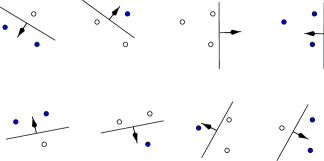
Figure 1: Example of an oriented line shattering 3 points. Solid and empty dots represent the two classes for $y$ and each of the $2^{3}$ permutations are shown.

Eq. 9 is a remarkable result which relates the number of training examples $l$, a fundamental property of the learning machine $h$, and the risk $R$ independent of the unknown distribution $p(x,y)$. The bounds provided by Eq. 9 are relatively weak due to their stunning generality.

It is important to realize that with an independent testing sample one can evaluate the true risk arbitrarily well. This testing sample, by definition, is not known to the algorithm, so the bound is useful for the design of algorithms through structural risk minimization. However, neural networks and most other methods rely on an independent testing sample to aid in their design and validation. An independent testing sample is clearly a better way to assess the true risk of a multivariate algorithm; however, Eq. 9 does shed light on the issues of overtraining, suggests the number of training samples that are needed, and offers a tool to compare different algorithms.

V.1 VC Dimension of Neural Networks

In order to apply Eq. 9, one must determine the VC dimension of neural networks. This is a difficult problem in combinatorics and geometry aided by algebraic techniques. Eduardo Sontag has an excellent review of these techniques and shows that the VC dimension of neural networks can, thus far, only be bounded fairly weakly Sontag . In particular, if we define $\rho$ as the number of weights and biases in the network, then the best bounds are $\rho^{2}<h<\rho^{4}$. In a typical particle physics neural network one can expect $100<\rho<1000$, which translates into a VC dimension as high as $10^{12}$, which implies $l>10^{13}$ for reasonable bounds on the risk. These bounds imply enormous numbers of training samples when compared to a typical training sample of $10^{5}$. Sontag goes on to show that these shattered sets are incredibly special and that the set of all shattered sets of cardinality $\mu>2\rho+1$ is measure zero in general. Thus, perhaps a more relevant notion of the VC dimension of a neural network is given by $\mu$.

VI Genetic Programming and Algorithms

Genetic Programming (GP) and Genetic Algorithms (GA) are based on a similar evolutionary metaphor in which “individuals” (potential solutions to the problem at hand) compete with respect to a user-defined performance measure. For new particle searches, the rate of Type II error, the significance, the exclusion potential, or G. Punzi’s suggestion Punzi are all reasonable performance measures. Ideally, one would use as a performance measure the same procedure that will be used to quote the results of the experiment. For instance, there is no reason (other than speed) that one could not include discriminating variables and systematic error in the optimization procedure (in fact, the author has done both).

The use of GP for the classification is fairly limited; however, it can be traced to the early works on the subject by Koza koza:gp . To the best of the author’s knowledge, the first application of GP within particle physics will appear in PhysicsGP . The difference between the algorithms is that GAs evolve a bit string which typically encodes parameters to a pre-existing program, function, or class of cuts, while GP directly evolves the programs or functions. For example, Field and Kanev Field:1997kt used Genetic Algorithms to optimize the lower- and upper-bounds for six 1-dimensional cuts on Modified Fox-Wolfram “shape” variables. In that case, the phase-space region was a pre-defined 6-cube and the GA was simply evolving the parameters for the upper- and lower-bounds. On the other hand, GP algorithm is not constrained to a pre-defined shape or parametric form. Instead, the GP approach is concerned directly with the construction of an optimal, non-trivial phase space region (i.e. an acceptance region $W$) with respect to a user-defined performance measure. GPs which only produce polynomial expressions form a vector space, which allows for a quick approximation of their VC dimension Sontag .

VII Conclusions

Clearly multivariate algorithms will have an increasingly important role in high energy physics, which necessitates that the field develop a coherent formalism and carefully consider what it means for a method to be optimal. Statistical learning theory offers a formalism that is general enough to describe all of the common multivariate analysis techniques, and provides interesting results relating risk, the number of training samples, and the learning capacity of the algorithm. However, independent testing samples and the global constraint on the rate of Type I error places some strain on the risk formalism. Finally, when one takes into account limited training data and systematic errors it is not clear that indirect methods are truly optimizing an experiments sensitivity. Direct methods, such as Genetic Programming, force analysts to be more clear about what statistical statements they plan to make and remove an artificial boundary between the goals of the experiment and the optimization procedures of the algorithm.

- [1] V. Vapnik and A.J. Cervonenkis. The uniform convergence of frequencies of the appearance of events to their probabilities. Dokl. Akad. Nauk SSSR, 1968. in Russian.
- [2] V. Vapnik. The Nature of Statistical Learning Theory. Springer, New York, 2nd edition, 2000.
- [3] J.K Stuart, A. Ord and S. Arnold. Kendall’s Advanced Theory of Statistics, Vol 2A (6th Ed.). Oxford University Press, New York, 1994.
- [4] Search for the standard model Higgs boson at LEP. Phys. Lett., B565:61–75, 2003.
- [5] D. Scott. Multivariate Density Estimation: Theory, Practice, and Visualization. John Wiley and Sons Inc., 1992.
- [6] K. Cranmer. Kernel estimation in high-energy physics. Comput. Phys. Commun., 136:198–207, 2001.
- [7] A. Askew. Event selection with adaptive gaussian kernels. In PhyStat2003, 2003.
- [8] L. Hölmstrom et. al. A new multivariate technique for top quark search. Comput. Phys. Commun., 88:195–210, 1995.
- [9] E. Sontag. VC dimension of neural networks. In C.M. Bishop, editor, Neural Networks and Machine Learning, pages 69–95, Berlin, 1998. Springer-Verlag.
- [10] G. Punzi. Sensitivity of searches for new signals and its optimization. In PhyStat2003, 2003.
- [11] J.R. Koza. Genetic Programming: On the Programming of Computers by Means of Natural Selection. MIT Press, Cambridge, MA, 1992.
- [12] K. Cranmer and R.S. Bowman. PhysicsGP: A genetic programming approach to event selection. submitted to Comput. Phys. Commun.
- [13] R. D. Field and Y. A. Kanev. Using collider event topology in the search for the six-jet decay of top quark antiquark pairs. hep-ph/9801318, 1997.