Frequentist Hypothesis Testing with Background Uncertainty

Abstract

We consider the standard Neyman-Pearson hypothesis test of a signal-plus-background hypothesis and background-only hypothesis in the presence of uncertainty on the background-only prediction. Surprisingly, this problem has not been addressed in the recent conferences on statistical techniques in high-energy physics – although the its confidence-interval equivalent has been. We discuss the issues of power, similar tests, coverage, and ordering rules. The method presented is compared to the Cousins-Highland technique, the ratio of Poisson means, and “profile” method.

I Introduction

In the last five years there have been several conferences on statistics for particle physics. Much of the emphasis of these conferences were on limit setting and the Feldman-Cousins “unified approach”, the quintessential frequentist method based on the Neyman construction. As particle physicists prepare for the Large Hadron Collider (LHC) at CERN, we will need to reexamine our list of statistical tools in the context of discovery. In fact, there has been no presentation at these statistical conferences on frequentist hypothesis testing in the presence of uncertainty on the background.

In Section II we will review the Neyman-Pearson theory for testing between two simple hypotheses, and examine the impact of background uncertainty in Section III. In Sections IV- V we will present a fully frequentist method for hypothesis testing with background uncertainty based on the Neyman Construction. In the remainder of the text we will present an example and compare this method to other existing methods.

II Simple Hypothesis Testing

In the case of Simple Hypothesis testing, the Neyman-Pearson theory (which we review briefly for completeness) begins with two Hypotheses: the null hypothesis $H_{0}$ and the alternate hypothesis $H_{1}$ Kendall . These hypotheses are called simple because they have no free parameters. Predictions of some physical observable $x$ can be made with these hypotheses and described by the likelihood functions $L(x|H_{0})$ and $L(x|H_{1})$ (for simplicity, think of $x$ as the number of events observed).

Next, one defines a region $W\in I$ such that if the data fall in $W$ we accept the $H_{0}$ (and reject $H_{1}$). Conversely, if the data fall in $I-W$ we reject $H_{0}$ and accept the $H_{1}$. The probability to commit a Type I error is called the size of the test and is given by

$$\alpha=\int_{I-W}L(x|H_{0})dx.$$ (1)

The probability to commit a Type II error is given by

$$\beta=\int_{W}L(x|H_{1})dx.$$ (2)

Finally, the Neyman-Pearson lemma tells us that the region $W$ of size $\alpha$ which minimizes the rate of Type II error (maximizes the power) is given by

$$W=\left\{x~{}\Bigg{|}~{}\frac{L(x|H_{1})}{L(x|H_{0})}>k_{\alpha}\right\}.$$ (3)

III Nuisance Parameters

Within physics, the majority of the emphasis on statistics has been on limit setting – which can be translated to hypothesis testing through a well known dictionary Kendall . When one includes nuisance parameters $\theta_{s}$ (parameters that are not of interest or not observable to the experimenter) into the calculation of a confidence interval, one must ensure coverage for every value of the nuisance parameter. When one is interested in hypothesis testing, there is no longer a physics parameter $\theta_{r}$ to cover, instead one must ensure the rate of Type I error is bounded by some predefined value. Analogously, when one includes a nuisance parameters in the null hypothesis, one must ensure that the rate of Type I error is bounded for every value of the nuisance parameter. Ideally one can find an acceptance region $W$ which has the same size for all values of the nuisance parameter (i.e. a similar test). Furthermore, the power of a region $W$ also depends on the nuisance parameter; ideally, we would like to maximize the power for all values of the nuisance parameter (i.e. Uniformly Most Powerful). Such tests do not exist in general.

In this note, we wish to address how the standard hypothesis test is modified by uncertainty on the background prediction. The uncertainty in the background prediction represents the presence of a nuisance parameter: for example, let us assume it is the expected background $b$. Typically, an auxiliary, or side-band, measurement is made to provide a handle on the nuisance parameter. Let us generically call that measurement $M$ and $L(M|H_{0},b)$ the prediction of that measurement given the null hypothesis with nuisance parameter $b$. In Section VIII we address the special case that $L(M|H_{0},b)$ is a Poisson distribution.

IV The Neyman-Construction

Usually one does not consider an explicit Neyman construction when performing hypothesis testing between two simple hypotheses; though one exists implicitly. Because of the presence of the nuisance parameter, the implicit Neyman construction must be made explicit and the dimensionality increased. The basic idea is that for each value of the nuisance parameters $\theta_{s}$, one must construct an acceptance interval (for $H_{0}$) in a space which includes their corresponding auxiliary measurements $M$, and the original test statistic $x$ which was being used to test $H_{0}$ against $H_{1}$.

For the simple case introduced in the previous section, this requires a three-dimensional construction with $b$, $M$, and $x$. For each value of $b$, one must construct a two-dimensional acceptance region $W_{b}$ of size $\alpha$ (under $H_{0}$). If an experiment’s data $(x_{0},M_{0})$ fall into an acceptance region $W_{b}$, then one cannot exclude the null hypothesis with $100(1-\alpha)\%$ confidence. Conversely, to reject the null hypothesis (i.e. claim a discovery) the data must not lie in any acceptance region $W_{b}$. Said yet another way, to claim a discovery, the confidence interval for the nuisance parameter(s) must be empty (when the construction is made assuming the null hypothesis).

V The Ordering Rule

The basic criterion for discovery was discussed abstractly in the previous section. In order to provide an actual calculation, one must provide an ordering rule: an algorithm which decides how to chose the region $W_{b}$. Recall, that there the constraint on Type I error does not uniquely specify an acceptance region for $H_{0}$. In the Neyman-Pearson lemma, it is the alternate hypothesis $H_{1}$ that breaks the symmetry between possible acceptance regions. Also in the unified approach, it is the likelihood ratio that is used as an ordering rule Feldman:1998qc .

At the Workshop on conference limits at FermiLab, Feldman showed that Unified Method with Nuisance Parameters is in Kendall’s Theory (the chapter on likelihood ratio tests & test efficiency) Feldman:fermilab . The notation used by Kendall is given in Table 1. Also, Kendall identifies $H_{0}$ with $\theta_{r}=\theta_{r0}$ and $H_{1}$ with $\theta_{r}\neq\theta_{r0}$.

Variable	Meaning
$\theta_{r}$	physics parameters
$\theta_{s}$	nuisance parameters
$\hat{\theta}_{r},\hat{\theta}_{s}$	unconditionally maximize $L(x|\hat{\theta}_{r},\hat{\theta}_{s})$
$\hat{\hat{\theta}}_{s}$	conditionally maximize $L(x|\theta_{r0},\hat{\hat{\theta}}_{s})$

Table 1: The notation used by Kendall for likelihood tests with nuisance parameters

Let us briefly quote from Kendall:

“Now consider the Likelihood Ratio

$$l=\frac{L(x|\theta_{r0},\hat{\hat{\theta}}_{s})}{L(x|\hat{\theta}_{r},\hat{\theta}_{s})}$$ (4)

Intuitively $l$ is a reasonable test statistic for $H_{0}$: it is the maximum likelihood under $H_{0}$ as a fraction of its largest possible value, and large values of $l$ signify that $H_{0}$ is reasonably acceptable.”

Feldman uses this chapter as motivation for the profile method (see Section IX), though in Kendall’s book the same likelihood ratio is used as an ordering rule for each value of the nuisance parameter.

The author tried simple variations on this ordering rule before rediscovering it as written. It is worth pointing out that Eq. 4 is independent of the nuisance parameter $b$; however, the contour of $l_{\alpha}$ which provides an acceptance region of size $\alpha$ is not necessarily independent of $b$. It is also worth pointing out that $\hat{\theta_{r}}$ and $\hat{\theta}_{s}$ do not consider the null hypothesis – if they did, the region in which $l=1$ may be larger than $(1-\alpha)$. Finally, if one uses $\theta_{s}$ instead of $\hat{\theta}_{s}$ or $\hat{\hat{\theta}}_{s}$, one will not obtain tests which are approximately similar.

VI An Example

Let us consider the case when the nuisance parameter is the expected number of background events $b$ and $M$ is an auxiliary measurement of $b$. Furthermore, let us assume that we have a absolute prediction of the number of signal events $s$. For our test statistic we choose the number of events observed $x$ which is Poisson distributed with mean $\mu=b$ for $H_{0}$ and $\mu=s+b$ for $H_{1}$. In the construction there are no assumptions about $L(M|H_{0},b)$ – it could be some very complicated shape relating particle identification efficiencies, Monte Carlo extrapolation, etc. In the case where $L(M|H_{0},b)$ is a Poisson distribution, other solutions exist (see Section VIII). For our example, let us take $L(M|H_{0},b)$ to be a Normal distribution centered on $b$ with standard deviation $\Delta b$, where $\Delta$ is some relative systematic error. Additionally, let us assume that we can factorize $L(x,M|H,b)=L(x|H,b)L(M|b)$ (where $H$ is either $H_{0}$ or $H_{1}$).

For our example problem, we can re-write the ordering rule in Eq. 4 as

$$l=\frac{L(x,M|H_{0},\hat{\hat{b}})}{L(x,M|H_{1},\hat{b})},$$ (5)

where $\hat{b}$ conditionally maximizes $L(x,M|H_{1},b)$ and $\hat{\hat{b}}$ conditionally maximizes $L(x,M|H_{0},b)$.

Now let us take $s=50$ and $\Delta=5\%$, both of which could be determined from Monte Carlo. In our toy example, we collect data $M_{0}=100$. Let $\alpha=2.85\cdot 10^{-7}$, which corresponds to $5\sigma$. The question now is how many events $x$ must we observe to claim a discovery? The condition for discovery is that $(x_{0},M_{0})$ do not lie in any acceptance region $W_{b}$. In Fig. 1 a sample of acceptance regions are displayed. One can imagine a horizontal plane at $M_{0}=100$ slicing through the various acceptance regions. The condition for discovery is that $x_{0}>x_{\rm max}$ where $x_{\rm max}$ is the maximal $x$ in the intersection.

There is one subtlety which arises from the ordering rule in Eq. 5. The acceptance region $W_{b}=\{(x,M)~{}~{}|~{}~{}l>l_{\alpha}\}$ is bounded by a contour of the likelihood ratio and must satisfy the constraint of size: $\int_{W_{b}}L(x,M|H_{0},b)=(1-\alpha)$. While it is true that the likelihood is independent of $b$, the constraint on size is dependent upon $b$. Similar tests are achieved when $l_{\alpha}$ is independent of $b$. The contours of the likelihood ratio are shown in Fig. 2 together with contours of $L(x,M|H_{0},b)$. While tests are roughly similar for $b\approx M$, similarity is violated for $M\ll b$. This violation should be irrelevant because clearly $b\ll M$ should not be accepted. This problem can be avoided by clipping the acceptance region around $M=b\pm N\Delta b$, where $N$ is sufficiently large ($\approx 10$) to have negligible affect on the size of the acceptance region. Fig. 1 shows the acceptance region with this slight modification.

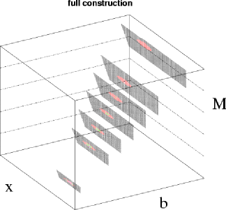
Figure 1: The Neyman construction for a test statistic $x$, an auxiliary measurement $M$, and a nuisance parameter $b$. Vertical planes represent acceptance regions $W_{b}$ for $H_{0}$ given $b$. The condition for discovery corresponds to data $(x_{0},M_{0})$ that do not intersect any acceptance region. The contours of $L(x,M|H_{0},b)$ are in color.

In the case where $s=50$, $\Delta=5\%$, and $M_{0}=100$, one must observe 167 events to claim a discovery. While no figure is provided, the range of $b$ consistent with $M_{0}=100$ (and no constraint on $x$) is $b\in[68,200]$. In this range, the tests are similar to a very high degree.

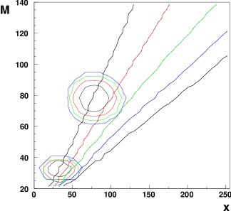
Figure 2: Contours of the likelihood $L(x,M|H_{0},b)$ are shown as concentric ellipses for $b=32$ and $b=80$. Contours of the likelihood ratio in Eq. 5 are shown as diagonal lines. This figure schematically illustrates that if one chooses acceptance regions based solely on contours of the likelihood ratio, that similarity is badly violated. For example, data $M=80,x=130$ would be considered part of the acceptance region for $b=32$, even though it should clearly be ruled out.

VII The Cousins-Highland Technique

The Cousins-Highland approach to hypothesis testing is quite popular FinalLHWG:2003sz because it is a simple smearing on the nuisance parameter Cousins:1992qz . In particular, the background-only hypothesis $L(x|H_{0},b)$ is transformed from a compound hypothesis with nuisance parameter $b$ to a simple hypothesis $L^{\prime}(x|H_{0})$ by

$$L^{\prime}(x|H_{0})=\int_{b}L(x|H_{0},b)L(b)db,$$ (6)

where $L(b)$ is typically a normal distribution. The problem with this method is largely philosophical: $L(b)$ is meaningless in a frequentist formalism. In a Bayesian formalism one can obtain $L(b)$ by considering $L(M|b)$ and inverting it with the use of Bayes’s theorem and the a priori likelihood for $b$. Typically, $L(M|b)$ is normal and one assumes a flat prior on $b$.

In the case where $s=50$, $L(b)$ is a normal distribution with mean $\mu=M_{0}=100$ and standard deviation $\sigma=\Delta M_{0}=5$, one must observe 161 events to claim a discovery. Initially, one might think that 161 is quite close to 167; however, they differ at the 4% level and the methods are only considering a $\Delta=5\%$ effect. Still worse, if $H_{0}$ is true (say $b_{t}=100$) and one can claim a discovery with the Cousins-Highland method ($x_{0}>161$), the chance that one could not claim a discovery with the fully frequentist method $(x_{0}<167$) is $\approx 95\%$. Similarly, if $H_{1}$ is true and one can claim a discovery with the Cousins-Highland method, the chance that one could not claim a discovery with the fully frequentist method is $\approx 50\%$. Even practically, there is quite a difference between these two methods.

VIII The Ratio of Poisson Means

During the conference, J. Linnemann presented results on the ratio of Poisson means. In that case, one considers a background and a signal process, both with unknown means. By making “on-source” (i.e. $x$) and “off-source” (i.e. $M$) measurements one can form a confidence interval on the ratio $\lambda=s/b$. If the $100(1-\alpha)\%$ confidence interval for $\lambda$ does not include $0$, then one could claim discovery. This approach does take into account uncertainty on the background; however, it is restricted to the case in which $L(M|b)$ is a Poisson distribution.

There are two variations on this technique. The first technique has been known for quite some time and was first brought to physics in Ref. James:1980 . This approach conditions on $x+M$, which allows one to tackle the problem with the use of a binomial distribution. Later, Cousins improved on these limits by removing the conditioning and considering the full Neyman construction Cousins:1998 . Cousins paper has an excellent review of the literature for those interested in this technique.

IX The Profile Method

As was mentioned in Section III the likelihood ratio in Eq. 4 is independent of the nuisance parameters. If it were not for the violations in similarity between tests, one would only need to perform the construction for one value of the nuisance parameters. Clearly, $\hat{\hat{\theta}}_{s}$ is an appropriate choice to perform the construction. This is the logic behind the profile method. It should be pointed out that the profile method is an approximation to the full Neyman construction; though a particularly good one. In the example above with $x_{0}=167$, $M_{0}=100$, the construction would be made at $b=\hat{\hat{b}}=117$ which gives the identical result as the fully frequentist method.

The main advantage to the profile method is that of speed and scalability. Instead of performing the construction for every value of the nuisance parameters, one must only perform the construction once. For many variables, the fully frequentist method is not scalable if one naïvely loops over on a fixed grid. However, Monte Carlo sampling the nuisance parameters does not suffer from the curse of dimensionality and serves as a more robust approximation of the full construction than the profile method.

X Conclusion

We have presented a fully frequentist method for hypothesis testing. The method consists of a Neyman construction in each of the nuisance parameters, their corresponding auxiliary measurements, and the test statistic that was originally used to test $H_{0}$ against $H_{1}$. We have chosen as an ordering rule the likelihood ratio with the nuisance parameters conditionally maximized to their respective hypotheses. With a slight modification, this ordering rule produces tests that are approximately similar. We have compared this method to the most common methods in the field. This method is philosophically more sound than the Cousins-Highland technique and more general than the ratio of Poisson means. This method can be made computationally less intensive either with Monte Carlo sampling of the nuisance parameters or by the approximation known as the profile method.

- [1] J.K Stuart, A. Ord and S. Arnold. Kendall’s Advanced Theory of Statistics, Vol 2A (6th Ed.). Oxford University Press, New York, 1994.
- [2] Gary J. Feldman and Robert D. Cousins. A unified approach to the classical statistical analysis of small signals. Phys. Rev., D57:3873–3889, 1998.
- [3] J. Feldman, Gary. Multiple measurements and parameters in the unified approach, 2000. Workshop on Confidence Limits, FermiLab.
- [4] Search for the standard model Higgs boson at LEP. Phys. Lett., B565:61–75, 2003.
- [5] R.D. Cousins and V.L. Highland. Incorporating systematic uncertainties into an upper limit. Nucl. Instrum. Meth., A320:331–335, 1992.
- [6] F. James and M. Roos. Errors on ratios of small numbers of events. Nucl. Phys., B 172:475–480, 1980.
- [7] R.D. Cousins. Improved central confidence intervals for the ratio of Poisson means. Nucl. Instrum. and Meth. in Phys. Res., A 417:391–399, 1998.