The Free Electron Laser Klystron Amplifier Concept

Abstract

The simplest high gain free electron laser (FEL) amplifier concept is proposed. A klystron amplifier has the useful property that the various electronic processes take place in separate portions of the amplifier, rather than overlapping as in FEL amplifier with an uniform undulator. The klystron consists of two fundamental parts: succession of 2-3 cascades (modulator), and an output undulator (radiator) in which the modulated electron beam coherently radiates. Each cascade consists of uniform undulator and dispersion section. Unlike distributed optical klystrons, we have a high gain per cascade pass. This has a few consequences. First, klystron gain does not depend on the bunch compression in the injector linac, i.e. maximum gain per cascade pass at high peak beam current is the same as at low peak beam current, without compression. Conventional, short-wavelength FEL amplifier and distributed optical klystron require electron beam peak current of a few kA. Second, there are no requirements on the alignment of the cascade undulators and dispersion sections, because, in our (high gain) case, there is no need for radiation phase matching. There are applications, like XFELs, where the unique properties of high gain klystron FEL amplifier are very desirable. Such a scheme allows one to decrease the total length of the magnetic system. In this paper we discuss also implementation of the proposed SASE FEL scheme for the frequency multiplier, for femtosecond experiments, and multi-user soft X-ray facility.

DESY 03-108

August 2003

, , and

1 Introduction

High gain FEL amplifiers are of interest for a variety of potential applications that range from X-ray lasers [1, 2] to ultraviolet MW-scale industrial lasers [3]. There are various versions of the high gain FEL amplifier. A number of high gain FEL amplifier concepts may prove useful for XFEL applications. Two especially noteworthy ones are the FEL amplifier with a single uniform undulator [1, 2] (see Fig. 1) and the distributed optical klystron [4, 5, 6, 7] (see Fig. 2). The high gain cascade klystron amplifier described in this paper is an attractive alternative to other configurations for operation in the X-ray wavelength range (see Fig. 3).

Let us first investigate qualitatively the processes that take place in any FEL amplifier; this investigation should also enable us to distinguish somewhat more accurately between the so-called distributed optical klystron concept and the new high gain klystron amplifier concept. In any FEL, several processes must take place, either separately or simultaneously. The first process that must occur in any FEL is energy modulation. Energy modulation means the application of radiation fields to the electrons as they move in their trajectories under the action of undulator magnetic fields, in such a way that the energies of these electrons are varied in some periodic fashion. It is then necessary to take advantage of this phase-dependent motion.

The second process, then, that must occure in a FEL is the conversion of this variation in the motion of the electrons into a usable form. It is necessary to turn the variations in the electron energy into a radiation frequency current, which can deliver energy to the electromagnetic field; i.e., the variations in velocity must be converted into density variations. The ways in which this conversion is brought about are numerous, and FEL amplifier types are distinguished by their conversion mechanism.

It may be useful to illustrate processes at this point to see how energy modulation and conversion into density modulation take place in some of the types of FEL amplifier. In a conventional high gain FEL amplifier with a single uniform undulator energy modulation and bunching occurs both simultaneously and continuously along the undulator. Energy modulation occurring at any one point continues to affect bunching at points beyond, with additional modulation being added as the beam moves along. The problem of electromagnetic wave amplification in the uniform undulator refers to a class of self-consistent problem. To solve the problem, the field equations and equations of particle motion should be solved simultaneously. When the FEL amplifier operates in linear regime the transverse distribution of the radiation field remains fixed, while its amplitude grows exponentially with undulator length.

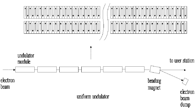
Figure 1: Schematic diagram of conventional SASE FEL

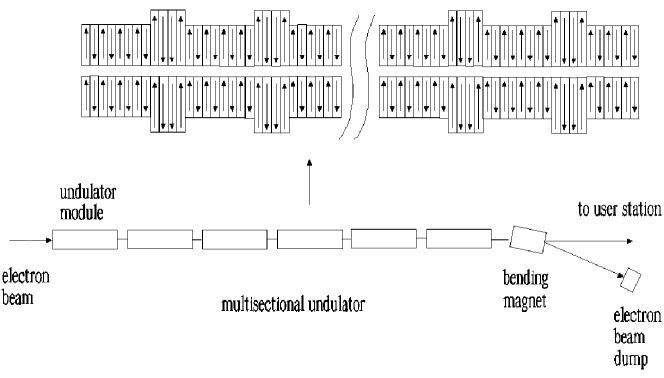
Figure 2: Schematic diagram of distributed optical klystron

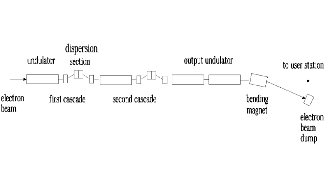
Figure 3: Schematic diagram of high gain cascade klystron amplifier

Perhaps the simplest FEL amplifier, from pedagogical point of view, is the high gain klystron amplifier. This simplicity arises from the fact that the important processes of energy modulation of the beam and subsequent conversion of the energy modulation to density modulation occur in distinctly separate regions of the FEL and thus may be considered in a sequential manner. This separability of functions aids materially in developing an understanding of modulation and bunching phenomena.

In its simplest configuration the klystron amplifier consists of an input undulator (energy modulator), and an output undulator (radiator) separated by a dispersion section. In the input undulator an incident electron beam is subjected to a radiation field, which produces an energy modulation, a modulation which after dispersion section, is converted into an density modulation in the beam. In the output undulator the bunched beam radiates coherently. This process, of conversion of energy modulation to bunching by the action of a dispersion section, is one of the characteristics of the klystron and is one of the reasons why this device is so useful in many connections.

We have considered the two-undulator klystron amplifier. In some experimental situations this simplest configuration is not optimal. For example, this study has shown that in the soft X-ray wavelength range the maximal (intensity) gain of this amplifier does not exceed 30-40 dB. The obvious and technically possible solution of the problem of gain increase might be to use a klystron with three or more undulators. Suppose that we have a three undulator (or so-called two-cascade) klystron, and that we introduce a very small signal into the first undulator. This will result in a small value of the amplitude of energy modulation, and a resulting rather small power output from the second undulator. Nevertheless, the radiation field amplitude in the second undulator will still be much greater than that in the first undulator, on account of the considerable amplification of the first cascade. We now disregard the power produced by the second undulator, but consider its effect on the electron beam passing through its magnetic system. The considerable radiation field in the second undulator will produce a further energy modulation of the beam and, when it emerges on the far side of the second undulator, it will have a large energy modulation, which, with a second dispersion section, will result in optimum bunching. This bunched beam then enters the third (radiator) undulator, and produces a large amount of power. In other words, we have essentially combined two stages of amplification by incorporating essentially two klystrons in a single unit. The final power is no greater than could be produced by a two-undulator klystron with the same output undulator, but we can secure this power with a much weaker input signal.

Let us consider now the problem of a periodically spaced sequence of undulators and dispersion sections, with the electron beam traversing each in succession. The larger the number of cascades the longer is the amplifier length. Suppose that the increase of total length (gain) of amplifier is tempered by an accompanying decrease in the length (gain) of cascade. From this approach at very large number of cascades and small gain per cascade pass we are led to the other device, which was the subject of the papers [4, 5, 6, 7]: the ”distributed optical klystron”. At first glance this is essentially the extension klystron amplifier, extended to a very large number of cascades. However, as noted earlier, this amplifier is considerably more complicated in principle than a klystron amplifier with high gain per cascade pass. When the gain per cascade pass is small, the cascades cannot be considered independent. It is important to realize that the cascades are connected optically, so that the radiation produced, for example, into the first undulator passes on into the second and produces additional energy modulation of the beam. It is clear that we cannot conveniently treat the theory of distributed klystron by the same method we used in the klystron case. Because of the low gain per cascade pass used for the distributed klystron, it cannot be approximated as scheme with separate functions, and the klystron amplifier theory has all based on that assumption. A quite different approach to the problem, which proves to be more suited to mathematical development of distributed klystron theory, is more along the lines of an analogy with the theory of conventional FEL amplifier with uniform undulator. The problem of electromagnetic wave amplification in the distributed klystron refers to a class of self-consistent problems. For instance, when the distributed klystron operates in linear regime its amplitude gain grows exponentially with cascade numbers. From a study of the rate of exponential build-up of the electromagnetic wave we can find the gain of the amplifier.

Our theory of klystron amplifier is based on the assumption that beam density modulation does not appreciably change as the beam propagates through the undulator. This approximation means that only the contributions to the radiation field arising from the initial density modulation are taken into account, and not those from the induced bunching. At very long klystron undulators we are led to device, which is the subject of the papers [8, 9]. Two-segment high gain FEL amplifier is variant of the standard high-gain FEL amplifier with uniform undulator. Because of the high gain per undulator pass used for this modification, it cannot be approximated as scheme with separate functions.

The klystron amplifier analysis is not only relevant from a pedagogical point of view. There are reasons to expect that the new concept of FEL amplifier discussed here can be of interest for short wavelength applications such as X-ray SASE FELs. Generation of X-ray radiation using klystron amplifiers has many advantages, primarily because of the separation of electronic processes, gain, and potentially low sensitivity to alignment. In principle, the gain of the klystron amplifier can be increased indefinitely by adding additional cascades along the beam. In practice, with three-cascade klystron amplifier, a gain in excess of 80 dB may be obtained in the soft X-ray wavelength range. At this level, the shot noise of the beam is amplified up to saturation and a cascade klystron amplifier operates as soft X-ray SASE FEL.

Now our intention is to develop certain physical ideas about the operation of the klystron amplifier, the characteristics of its radiation, and those features that set it apart from other FEL sources in the short wavelength region of the spectrum. The resonance properties of the radiation of the electron beam in the klystron can be understood as follows. Since a dispersion section is a nonresonant device, the klystron bandwidth is restricted by the resonance properties of the cascade undulator, that is, by its number of periods $N_{\mathrm{w}}$. The typical amplification bandwidth of the klystron in the soft X-ray wavelength range is on the order of one percent $(N_{\mathrm{w}}\simeq 10^{2})$. Since we study the start-up from shot noise, we assume the input current to have a homogeneous spectral distribution. At large number of undulator periods the spectrum of transversely coherent fraction of radiation is concentrated within the narrow band, $\Delta\lambda/\lambda\simeq N^{-1}_{\mathrm{w}}$.

The actual physical picture of start-up from noise should take into account that the fluctuations of current density in the electron beam are uncorrelated not only in time but in space too. Thus a large number of transverse radiation modes are excited when the electron beam enters the undulator. These radiation modes have different gain. Obviously, as cascade number progresses, the high gain modes will predominate more and more and we can regard the klystron as a filter, in the sense that it filters from arbitrary radiation field those components corresponding to the high gain modes. If we consider the undulator radiation from the point of view of paraxial optics, then we immediately see that the high gain modes are associated with radiation propagating along the axis of the undulator, as opposed to radiation propagating at an angle to the axis which has a low gain. Consider an electron beam of radius $r_{\mathrm{b}}$ moving in the (cascade) undulator with length $L_{\mathrm{w}}$. The parameter $N_{\mathrm{F}}=r_{\mathrm{b}}^{2}/(\lambda L_{\mathrm{w}})$ can be referred to as the Fresnel number. Here $\lambda$ is the radiation wavelength. The requirement for the mode selection to be quickly holds at small value of the Fresnel number. Hence, for thin electron beam with Fresnel number of $N_{\mathrm{F}}\simeq 1$, the emission will emerge in a single (fundamental) transverse mode and the degree of transverse coherence of output radiation will approach unity.

As mentioned above, amplification in each cascade is a two-step process. Since we study the start-up from shot noise there is no electromagnetic field at the undulator entrance and the modulation of the beam density serves as the input signal for the klystron amplifier. The radiation field produced an ponderomotive potential across the undulator; as is now known from general FEL theory, this voltage modulates the energy of the electron beam. Then the energy modulation causes modulation of the beam density in the dispersion section. If we can neglect beam bunching in the cascade undulator, the amplitude of energy modulation at the undulator exit, $\delta{\cal E}$, is proportional to the resonance Fourier component of beam current, $\delta I_{\mathrm{in}}=a_{\mathrm{in}}I_{0}$. Here $a_{\mathrm{in}}$ is the initial beam microbunching at the resonant wavelength, and $I_{0}$ is the peak beam current. We now examine the behaviour of the electrons as they travel in a dispersion section. Like the situation with usual microwave klystron, the Bessel function factor $J_{1}(X)$ represents the microbunching at the dispersion section exit. The parameter $X$ in our case is proportional to the product of the amplitude of energy modulation $\delta{\cal E}$ and the compaction factor of the dispersion section $R_{56}$. In the high gain linear regime $X$ is much smaller then unity and we make the approximation $J_{1}(X)\simeq X/2$. Thus, microbunching at the cascade exit is proportional to input signal amplitude, $a_{\mathrm{out}}\sim R_{56}I_{0}a_{\mathrm{in}}$. When a cascade operates in the high gain linear regime the gain per cascade pass is independent of input signal amplitude and proportional to the product of the compaction factor and the peak beam current, $G=a_{\mathrm{out}}/a_{\mathrm{in}}\sim R_{56}I_{0}$.

If we build a klystron, we want to have small number of cascades and high gain. One might think that all we have to do is to get enough gain per cascade pass - we can always increase compaction factor $R_{56}$ and we can always increase $G$, and there is no reason why we cannot use the simple two-undulator klystron scheme. So the limitations of a gain per cascade pass are not that it is impossible to build a dispersion section that has a very large compaction factor. In fact, one of the main problems in klystron amplifier operation is preventing spread of microbunching due to energy spread into the electron beam. This energy spread is unimportant when the compaction factor of dispersion section is relatively small, but we shell see that energy spread is of fundamental importance in the case of very large compaction factor. To get a rough idea of the spread of the microbunching, the position of the particles within the electron bunch at the dispersion section exit has a spread which is equal to $\Delta z\simeq R_{56}\Delta\gamma/\gamma$, where $\Delta\gamma/\gamma$ is the local energy spread into the electron beam. And how big is $\Delta z$ in the spread-out microbunching? We know that uncertainty in the phase of the particles is about $\Delta\psi\simeq 2\pi\Delta z/\lambda$. Therefore, the largest compaction factor that we can have is approximately $R_{56}\simeq\lambda\gamma/(2\pi\Delta\gamma)$. This is what we wanted to deduce - that the gain maximum per cascade pass varies as ratio $G_{\mathrm{max}}\sim I_{0}/\Delta\gamma$. It is of course desirable that the klystron gain be maximum. An experimenter can easily tune the gain of the klystron by tuning the magnetic fields in the dispersion sections. It should be pointed out that the local energy spread plays a very important role in the operation of the FEL klystron amplifier, and this characteristic distinguishes the klystron from conventional FEL amplifier.

Electron bunches with very small transverse emittance and high peak current are needed for the operation of conventional XFELs. This is achieved using a two-step strategy: first generate beams with small transverse emittance using an RF photocathode and, second, apply longitudinal compression at high energy using a magnetic chicane. Although simple in first-order theory, the physics of bunch compression becomes very challenging if collective effects like space charge forces and coherent synchrotron radiation forces (CSR) are taken into account. Wakefields of bunches as short as 0.1 mm have never been measured and are challenging to predict.

The situation is quite different for klystron amplifier scheme described in our paper. An distinguishing feature of the klystron amplifier is the absence of apparent limitations which would prevent operation without bunch compression in the injector linac. According to our discussion above, the gain maximum per cascade pass is proportional to the peak current and inversely proportional to the energy spread of the beam. Since the bunch length and energy spread are related to each other through Liouville’s theorem, the peak current and energy spread cannot vary independently of each other in the injector linac. To extent that local energy spead is proportional to the peak current, which is usually the case for bunch compression, the gain will be independent of the actual peak current. We see, therefore, that klystron gain in linear regime depends only on the actual photoinjector parameters. This incipient proportionality between gain and $I_{0}/\Delta\gamma$ is a temptation, in designing an XFEL, to go to very high values of $I_{0}/\Delta\gamma$ and very long values of bunch length.

Let us present a specific numerical example for the case of a 4th generation soft X-ray light source based on the use RF photoinjector and superconducting linac with duty factor 1 %. The average brilliance of a klystron facility operating without bunch compression in the injector linac surpasses the spontaneous undulator radiation from 3rd generation synchrotron radiation facilities by 4 or more orders of magnitude. Decreasing the peak current also decreases the peak brilliance of the SASE FEL radiation by about of factor 100, but this is still 6 order of magnitude higher than that of 3rd generation synchrotron radiation sources.

Our studies have shown that the soft X-ray cascade klystron holds great promise as a source of radiation for generating high power single femtosecond pulses. The obvious temporal limitation of the visible pump/X-ray probe technique is the duration of the X-ray probe. At a klystron facility operating without bunch compression, the X-ray pulse duration is about 10 ps. This is longer than the timescale of many interesting physical phenomena. The new principle of pump-probe techniques described in section 6 offers a way around this difficulty. Section 6 also deals with the design strategy for the multi-user distribution system for an X-ray laboratory. An X-ray laboratory should serve several, may be up to ten experimental stations which can be operated independently according to the needs of the user community. On the other hand, the prefered layout of a conventional SASE FEL is a linear arrangement in which the injector , accelerator, bunch compressors and undulators are nearly collinear, and in which the electron beam does not change direction between accelerator and undulators. The situation is quite different for the klystron amplifier scheme proposed in our paper. Since it operates without bunch compression in the injector linac, the problem of emittance dilution in the bending magnets does not exist. An electron beam distribution system based on unbunched electron beam can provide efficient ways to generate a multi-user facility - very similar to present day synchrotron radiation facilities.

It may be wondered, after hearing of all of the wonderful properties of the high gain klystron amplifier, why this advance in XFEL techniques occurred only this year. It should be note that the XFEL which was proposed in 1982 [10] has had nearly 20 years of development. One of the explanations is as follows. For years we were led to believe that local energy spread into electron beam which delivered from a photoinjector is relatively large. Recent analysis of experimental results obtained at TTF SASE FEL [11] shows that the value of the local energy spread should be revised. After bunch compression, it is expected to be about 0.2 MeV (for $I_{0}\simeq 2.5\ {\mathrm{kA}}$) or smaller which is significantly less than the previously projected value of 1 MeV. This decrease significantly improves operation of klystron amplifier and extends the safety margin for X-ray klystron facility operation.

This paper is intended primarily for the experimental scientist or XFEL program manager who has to design XFELs and who wishes to undestand the operating principles of XFELs. The material to be discussed provides the necessary background information required for making strategic XFEL design decisions. In this paper the electronic processes that occur in an XFEL will be discussed in elementary fashion. The XFEL theory has a, not entirely undeserved, reputation for difficulty and obscurity. This is due partly to the complexity of systems in which (shot) noise is input signal and partly to the unfamiliar nature of some of the mathematical tools involved (integrodifferential equations). Klystron amplifiers are one of the simplest examples of high gain FEL amplifiers and therefore we shall use them as an introduction to the techniques of XFEL theory. In the klystron amplifier case little demand is made on the reader’s mathematical ability. The mathematics that is involved is particularly simple, involving very simple differential equations and algebraic operations and no integrodifferential equations. Such introduction to the operating principles of XFELs has never been done before, to our knowledge.

2 Interaction between electrons and fields in an undulator

Klystron amplifiers amplify the input signal. To describe the klystron amplifier operation, we first define the initial conditions. Important practical kind of initial condition refers to the case when there is no radiation field at the undulator entrance and the modulation of the beam current density serves as the input signal for the amplifier. As stated in the introductory section, in undulator two physical processes take place simultaneously:

1) The modulated electron beam excites electromagnetic waves which are propagated along the undulator;

2) The electric field components of these waves produce a modulation of the energy of the electrons.

The approach discussed in this section consists of deriving for these two process separate expressions which, when joined, give quantitative information about the composite phenomena taking place in the undulator. We assume that the density modulation effect is negligible. Hence, electrons passing through the first undulator receive only energy modulation, but no density modulation. Density modulation present when the electrons enter the second undulator, must have developed while the electrons were traveling in the dispersion section. This effect will be discussed later.

2.1 Collective fields produced by the modulated electron beam in an undulator

The simplest form of bunched beam is found if we have swarm of electrons, all moving in the same direction (say the $z$-direction) with the same velocity (say $v$), but in which the number of electrons per unit volume (say $n$) depends on $z$. Then if the charge on the electron $(-e)$ we can easily find the current density at any value of $z$. The quantity $n$ must really be a function of $z/v-t$, on account of the velocity $v$ of the electrons. Thus, the current density at point $z$, at time $t$, is $-ev_{z}n(z/v-t)$, where $n(z/v-t)$ indicates the function $n$ of the argument $z/v-t$. Unless $n$ is a constant independent of its argument, this will lead to a current density which varies with time. The simplest variation of $n$ for our present purposes is a superposition of a constant, or d-c component, and a periodic function of $z/v-t$, with an angular frequency $\omega$. First we consider the case where $n$ is simply a constant plus a single cosine term: $n(z/v-t)=n_{0}[1+a_{\mathrm{in}}\cos\omega(z/v-t)]$. We must note one important fact: $n$ can never become negative, and hence $a_{\mathrm{in}}$ cannot be greater than unity.

To understand the basic principles of klystron amplifier operation, let us consider the helical undulator. The magnetic field on the axis of the helical undulator is given by

$$\vec{H}_{\mathrm{w}}=\vec{e}_{x}H_{\mathrm{w}}\cos(k_{\mathrm{w}}z)-\vec{e}_{y}H_{\mathrm{w}}\sin(k_{\mathrm{w}}z)\ ,$$

where $k_{\mathrm{w}}=2\pi/\lambda_{\mathrm{w}}$ is the undulator wavenumber and $\vec{e}_{x,y}$ are unit vectors directed along the $x$ and $y$ axes of the Cartesian coordinate system $(x,y,z)$. The Lorentz force $\vec{F}=-e(\vec{v}\times\vec{H}_{\mathrm{w}})/c$ is used to derive the equations of motion of electrons with charge $(-e)$ and mass $m_{\mathrm{e}}$ in the presence of the magnetic field. The explicit expression for the electron velocity in the field of the helical undulator has the form:

$$\vec{v}_{\perp}(z)=c\theta_{\mathrm{w}}\left[\vec{e}_{x}\cos(k_{\mathrm{w}}z)-\vec{e}_{y}\sin(k_{\mathrm{w}}z)\right]\ ,$$

which means that the electron in the undulator moves along a constrained helical trajectory parallel to the $z$ axis. The angle of rotation is given by the relation $\theta_{\mathrm{w}}=K/\gamma=\lambda_{\mathrm{w}}eH_{\mathrm{w}}/(2\pi m_{\mathrm{e}}c^{2}\gamma)$, where $\gamma=(1-v^{2}/c^{2})^{-1/2}$ is the relativistic factor and $v^{2}=v_{x}^{2}+v_{y}^{2}+v_{z}^{2}$. As a rule, the electron rotation angle $\theta_{\mathrm{w}}$ is small and the longitudinal electron velocity $v_{z}$ is close to the velocity of light, $v_{z}\simeq c$.

Let us consider a bunched relativistic electron beam moving along the $z$ axis in the field of a helical undulator. In what follows we use the following assumptions: i) the electrons move along constrained helical trajectories in parallel with the $z$ axis; ii) the radius of the electron rotation in the undulator, $r_{\mathrm{w}}=\theta_{\mathrm{w}}/k_{\mathrm{w}}$, is much less than the transverse size of the electron beam. Next let us assume that electron beam density at the undulator entrance is simply $n=n_{0}(\vec{r}_{\perp})[1+a_{\mathrm{in}}\cos\omega(z/v_{z}-t)]$, where $a_{\mathrm{in}}={\mathrm{const.}}$ In other words we consider the case in which there are no variations in amplitude and phase of the density modulation in the transverse plane.

Under these assumptions the transverse current density may be written in the form

$$\vec{j}_{\perp}=-e\vec{v}_{\perp}(z)n(\vec{r}_{\perp},z/v_{z}-t)=-e\vec{v}_{\perp}n_{0}(\vec{r}_{\perp})[1+a_{\mathrm{in}}\cos\omega(z/v_{z}-t)]\ ,$$

where we calibrated the time in such a way that current density has its maximum at time $t=0$, at point $z=0$. Even through the measured quantities are real, it is generally more convenient to use complex representation. For this reason, starting with real $\vec{j}_{\perp}$, one defines the complex transverse current density:

$$j_{x}+\mathop{\mathrm{i}}j_{y}=-ec\theta_{\mathrm{w}}n_{0}(\vec{r}_{\perp})\exp(-\mathop{\mathrm{i}}k_{\mathrm{w}}z)[1+a_{\mathrm{in}}\cos\omega(z/v_{z}-t)]\ .$$ (1)

Transverse current have the angular frequency $\omega$ and two waves traveling in the same directions with variations $\exp\mathop{\mathrm{i}}(\omega z/v_{z}-k_{\mathrm{w}}z-\omega t)$ and $\exp-\mathop{\mathrm{i}}(\omega z/v_{z}+k_{\mathrm{w}}z-\omega t)$ will add to give a total current proportional to $\exp(-\mathop{\mathrm{i}}k_{\mathrm{w}}z)\cos\omega(z/v_{z}-t)$. The factor $\exp\mathop{\mathrm{i}}(\omega z/v_{z}-k_{\mathrm{w}}z-\omega t)$ indicates a fast wave, while the factor $\exp-\mathop{\mathrm{i}}(\omega z/v_{z}+k_{\mathrm{w}}z-\omega t)$ indicates a slow wave. The use of the word ”fast” (”slow”) here implies a wave with a phase velocity faster (slower) than the beam velocity.

Now we should consider the electrodynamic problem. Using Maxwell’s equations, we can write the equation for the electric field:

$$c^{2}\vec{\nabla}\times(\vec{\nabla}\times\vec{E})=-\partial^{2}\vec{E}/\partial t^{2}-4\pi\partial\vec{j}/\partial t\ .$$

Then make use of the identity

$$\vec{\nabla}\times(\vec{\nabla}\times\vec{E})=\vec{\nabla}(\vec{\nabla}\cdot\vec{E})-\vec{\nabla}^{2}\vec{E}\ ,$$

where $\vec{\nabla}\cdot\vec{E}$ can be found from the Poisson equation. Finally, we come to the inhomogeneous wave equation for $\vec{E}$:

$$c^{2}\vec{\nabla}^{2}\vec{E}-\partial^{2}\vec{E}/\partial t^{2}=4\pi c^{2}\vec{\nabla}\rho+4\pi\partial\vec{j}/\partial t\ .$$ (2)

This equation allows one to calculate the electric field $\vec{E}(\vec{r},t)$ for given charge and current sources, $\rho(\vec{r},t)$ and $\vec{j}(\vec{r},t)$. Thus, equation (2) is the complete and correct formula for radiation. However we want to apply it to a still simpler circumstance in which the second term (or, the current term) in the right-hand side of (2) provides the main contribution to the value of the radiation field. Since in the paraxial approximation the radiation field has only transverse components, we are interested in the transverse component of (2). Thus we consider the wave equation

$$c^{2}\vec{\nabla}^{2}\vec{E}_{\perp}-\partial^{2}\vec{E}_{\perp}/\partial t^{2}=4\pi\partial\vec{j}_{\perp}/\partial t\ ,$$ (3)

which relates the transverse component of the electric field to the transverse component of current density.

We wish to examine the case when the phase velocity of the current wave is close to the velocity of light. This requirement may be met under resonance condition

$$\omega/c=\omega/v_{z}-k_{\mathrm{w}}\ .$$ (4)

First we may point out that the statement of (4), the condition for the relation between $\omega,k_{\mathrm{w}}$ and $v_{z}$, is the condition for synchronism between the transverse electromagnetic wave and the fast transverse current wave with the propagating constant $\omega/v_{z}-k_{\mathrm{w}}$. With a current wave traveling with the same phase speed as the electromagnetic wave, we have the possibility of (space) resonance between electromagnetic wave and electrons. If this is the case cumulative interaction between bunched electron beam and transverse electromagnetic wave takes place. We are therefore justified in considering the contributions of all the waves except the synchronous one to be negligible.

It would be nice to find an explanation of resonance condition (4) which is elementary in the sense that we can see what is happening physically. Let us call the plane electromagnetic wave velocity $c$, which is of course, related to the phase constant by $k=\omega/c$. Then the velocity of the beam relative to the electromagnetic wave is merely $c-v_{z}$. With this relative velocity, the frequency of the electromagnetic waves as seen by the electrons is give by $\omega_{\mathrm{e}}=(c-v_{z})k$, where we have used the obvious relation between the phase constant $k$ and the wavelength of the electromagnetic wave, $k=2\pi/\lambda$. Relation for $\omega_{\mathrm{e}}$ can be written as $\omega_{\mathrm{e}}=\omega-kv_{z}$. Under the condition when (4) holds, we see by comparison with that equation that this would be merely the undulator frequency $\omega_{\mathrm{e}}=k_{\mathrm{w}}v_{z}$. Accordingly, the condition of (4) that we have imposed is merely that the electron velocity is such that as the electron run past the electromagnetic waves, the apparent frequency they see is the undulator frequency. This is the basic effect involved in this interaction. If the apparent frequency is the undulator frequency, a cumulative effect on the electromagnetic wave results, since the waves are being driven at a frequency corresponding to natural rotation frequency of the electrons in the magnetic field. Another way of saying the same thing is that in the frame of reference moving with the electrons, the electromagnetic waves have a Doppler-shifted frequency equal to undulator frequency.

Any state of transverse electromagnetic wave can always be written as a linear combination of the two base states (polarizations). By giving the amplitudes and phases of these base states we completely describe the electromagnetic wave state. It is usually best to start with the form which is physically clearest. We choose the Cartesian base states and seek the solution for $\vec{E}_{\perp}$ in the form

$$E_{x,y}=\tilde{E}_{x,y}(z,\vec{r}_{\perp})\exp[\mathop{\mathrm{i}}\omega(z/c-t)]+{\mathrm{C.C.}}$$ (5)

Here and in what follows, complex amplitudes related to the field are written with a tilde. The description of the field given by (5) is quite general. However, the usefulness of the concept of carrier wave number is limited to the case where the amplitude is slowly varying function of $z$.

To determine the form of $\tilde{E}_{x,y}(z,\vec{r}_{\perp})$ we substitute (1) and (5) into (3). We have

$$\exp[\mathop{\mathrm{i}}\omega(z/c-t)]\left\{\vec{\nabla}^{2}_{\perp}+\frac{2\mathop{\mathrm{i}}\omega}{c}\frac{\partial}{\partial z}+\frac{\partial^{2}}{\partial z^{2}}\right\}{\tilde{E}_{x}\choose\tilde{E}_{y}}+{\mathrm{C.C.}}$$

$$=-4\pi\frac{\omega}{c}{\cos(k_{\mathrm{w}}z)\choose-\sin(k_{\mathrm{w}})}e\theta_{\mathrm{w}}a_{\mathrm{in}}n_{0}(\vec{r}_{\perp})\sin\omega(z/v_{z}-t)\ .$$ (6)

Here $\vec{\nabla}^{2}_{\perp}$ is the Laplace operator in transverse coordinates.

Now we have an apparently simple pair of equations - and they are still exact, of course. The question is, how to solve these equations? First we simplify the equations obtained by noting that for a radiation field it is reasonable to assume that $\tilde{E}_{x,y}(z,\vec{r}_{\perp})$ are slowly varying functions of $z$ (because of the radiation directivity) so that $\partial^{2}\tilde{E}_{x,y}/\partial z^{2}$ may be neglected. The corresponding requirement for the complex amplitude is $\mid\partial\tilde{E}_{x,y}/\partial z\mid\ll k\mid\tilde{E}_{x,y}\mid$. In other words, the radiation pulse must not change significantly while traveling through a distance comparable with the wavelength $\lambda=2\pi/k$. This assumption is not a restriction. Such is the case in all practical cases of interest. Differential equations becomes

$$\exp[\mathop{\mathrm{i}}\omega(z/c-t)]\left\{\vec{\nabla}^{2}_{\perp}+\frac{2\mathop{\mathrm{i}}\omega}{c}\frac{\partial}{\partial z}\right\}{\tilde{E}_{x}\choose\tilde{E}_{y}}+{\mathrm{C.C.}}$$

$$=4\pi\frac{\omega}{c}{\cos(k_{\mathrm{w}}z)\choose-\sin(k_{\mathrm{w}})}e\theta_{\mathrm{w}}a_{\mathrm{in}}n_{0}(\vec{r}_{\perp})\sin\omega(t-z/v_{z})\ .$$ (7)

The reader may well wonder why such a transformation is useful; therefore we digress temporarily to address this question.

Such a transformation immediately modifies the hyperbolic wave equations to the parabolic equations. We should stress that the equations (7) are preferable for an analytical solution, since the mathematical techniques are always connected with more conventional parabolic equations. Although equations (7) cannot be solved in general, we will solve them for some special cases. These equations can be simplified further by noting that the complex amplitudes $\tilde{E}_{x,y}$ will not vary much with $z$, especially in comparison with the exponential terms $\exp(-\mathop{\mathrm{i}}k_{\mathrm{w}}z)$. The slow wave of transverse current oscillates very rapidly about an average value of zero and, therefore, does not contribute very much to the rate of change of $\tilde{E}_{x,y}$. So we can make a reasonably good approximation by replacing these terms by their average value, namely, zero. We will leave them out, and take as our approximation:

$$\vec{\nabla}^{2}_{\perp}{\tilde{E}_{x}\choose\tilde{E}_{y}}+\frac{2\mathop{\mathrm{i}}\omega}{c}\frac{\partial}{\partial z}{\tilde{E}_{x}\choose\tilde{E}_{y}}=-{\mathop{\mathrm{i}}\choose 1}2\pi\frac{\omega}{c}e\theta_{\mathrm{w}}a_{\mathrm{in}}n_{0}(\vec{r}_{\perp})\exp(-\mathop{\mathrm{i}}Cz)\ .$$ (8)

Even the remaining terms, with exponents proportional to $C=\omega/v_{z}-\omega/c-k_{\mathrm{w}}$ will also vary rapidly unless $C$ is near zero. Only then will the right-hand side vary slowly enough that any appreciable amount will accumulate when we integrate the equations with respect to $z$. The required conditions will be met if

$$C\ll k_{\mathrm{w}}\qquad 1\ll k_{\mathrm{w}}z\ .$$

In other words, we use the resonance approximation here and assume that complex amplitudes $\tilde{E}_{x,y}$ are slowly varying in the longitudinal coordinate. By ”slowly varying” we mean that $\mid\partial\tilde{E}_{x,y}/\partial z\mid\ll k_{\mathrm{w}}\mid\tilde{E}_{x,y}\mid$. For this inequality to be satistied, the spatial variation of $\tilde{E}_{x,y}$ within an undulator period $\lambda_{\mathrm{w}}=2\pi/k_{\mathrm{w}}$ has to be small.

Equations (8) are simple enough and can be solved in any number of ways. One convenient way is the following. Taking the sum and the difference of the two we get

$$\left(\vec{\nabla}^{2}_{\perp}+\frac{2\mathop{\mathrm{i}}\omega}{c}\frac{\partial}{\partial z}\right)\left(\tilde{E}_{x}+\mathop{\mathrm{i}}\tilde{E}_{y}\right)=2\pi\mathop{\mathrm{i}}\frac{\omega}{c}e\theta_{\mathrm{w}}a_{\mathrm{in}}n_{0}(\vec{r}_{\perp})\exp(-\mathop{\mathrm{i}}Cz)\ ,$$ (9)

$$\left(\vec{\nabla}^{2}_{\perp}+\frac{2\mathop{\mathrm{i}}\omega}{c}\frac{\partial}{\partial z}\right)\left(\tilde{E}_{x}-\mathop{\mathrm{i}}\tilde{E}_{y}\right)=0\ .$$ (10)

These equations describe the general case of electromagnetic wave radiation by the bunched electron beam in the helical undulator. Equation (9) and (10) refer to the right- and left-helicity components of the wave respectively. The solutions for the right- and left-helicity waves are linearly independent . It follows from (9) and (10) that only those waves are radiated that have the same helicity as the undulator field itself.

Of course we could predict such a result. The electric field, $\vec{E}_{\perp}$, of the wave radiated in the helical undulator in resonance approximation is circularly polarized and may be represent in the complex form:

$$E_{x}+\mathop{\mathrm{i}}E_{y}=\tilde{E}(z,\vec{r}_{\perp})\exp[\mathop{\mathrm{i}}\omega(z/c-t)]\ .$$ (11)

Finally, the equation for $\tilde{E}$ can be written in the form

$$\left(\vec{\nabla}^{2}_{\perp}+\frac{2\mathop{\mathrm{i}}\omega}{c}\frac{\partial}{\partial z}\right)\tilde{E}=2\pi\mathop{\mathrm{i}}\frac{\omega}{c}e\theta_{\mathrm{w}}a_{\mathrm{in}}n_{0}(\vec{r}_{\perp})\exp(-\mathop{\mathrm{i}}Cz)\ .$$ (12)

Equation (12) is an inhomogeneous parabolic equation. Its solution can be expressed in terms of a convolution of the free-space Green’s function (impulse response)

$$G(z-z^{\prime},\vec{r}_{\perp}-\vec{r}^{\prime}_{\perp})=\frac{1}{4\pi(z-z^{\prime})}\exp\left[\frac{\mathop{\mathrm{i}}\omega\mid\vec{r}_{\perp}-\vec{r}^{\prime}_{\perp}\mid^{2}}{2c(z-z^{\prime})}\right]\$$ (13)

with the source term. When the right-hand side of (12) is equal to zero, it transforms to the well-known paraxial wave equation in optics.

The radiation process displays resonance behaviour and the amplitude of electric field depends stronly on the value of the detuning parameter $C$. With the approximation made in getting (12) the equation can be solved exactly, but the work is a little elaborate, so we won’t do that until later when we take up the problem of output radiation characteristics. Now we will find an exact solution for the case of perfect resonance. When the parameters are tuned to perfect resonance, such that $C=0$, the solution of the equation (12) has the form

$$\tilde{E}(z,\vec{r}_{\perp})=\frac{\mathop{\mathrm{i}}e\theta_{\mathrm{w}}\omega a_{\mathrm{in}}}{2c}\int\limits^{z}_{0}\frac{\mathop{\mathrm{d}}z^{\prime}}{z-z^{\prime}}\int\mathop{\mathrm{d}}\vec{r}^{\prime}_{\perp}n_{0}(\vec{r}_{\perp}^{\prime})\exp\left[\frac{\mathop{\mathrm{i}}\omega\mid\vec{r}_{\perp}-\vec{r}^{\prime}_{\perp}\mid^{2}}{2c(z-z^{\prime})}\right]\ ,$$ (14)

where $(z,\vec{r}_{\perp})$ and $(z^{\prime},\vec{r}_{\perp}^{\prime})$ are the coordinates of the observation and the source point, respectively.

Let us consider an axisymmetric electron beam with gradient profile of the current density. In this case we have $-ev_{z}n_{0}(\vec{r}_{\perp})=-j_{0}S(r)$, where $r$ is the radial coordinate of the cylindrical system $(r,\phi,z)$ and $S(r)$ describes the transverse profile of the electron beam. To be specific, we write down all the expressions for the case of a Gaussian transverse distribution:

$$-ev_{z}n_{0}(\vec{r}_{\perp})=-j_{0}S(r)=-\frac{I_{0}}{2\pi\sigma^{2}}\exp\left(-\frac{r^{2}}{2\sigma^{2}}\right)\ ,$$

where $I_{0}$ is the total beam current. At this point we find it convenient to impose the following restriction: we focus only on the radiation see by an observer lying on the electron beam axis. When $r=0$ and the beam profile is Gaussian, we can write (14) in the form

$$\tilde{E}_{0}(z)=\frac{\mathop{\mathrm{i}}\theta_{\mathrm{w}}\omega a_{\mathrm{in}}I_{0}}{2\sigma^{2}c^{2}}\int\limits^{z}_{0}\frac{\mathop{\mathrm{d}}z^{\prime}}{z-z^{\prime}}\int\limits^{\infty}_{0}r^{\prime}\exp\left[-\frac{(r^{\prime})^{2}}{2\sigma^{2}}\right]\exp\left[\frac{\mathop{\mathrm{i}}\omega(r^{\prime})^{2}}{2c(z-z^{\prime})}\right]\mathop{\mathrm{d}}r^{\prime}\ .$$

Integrating first with respect to $r^{\prime}$, we have

$$\tilde{E}_{0}(z)=\frac{\mathop{\mathrm{i}}\theta_{\mathrm{w}}\omega a_{\mathrm{in}}I_{0}}{2c^{2}}\int\limits^{z}_{0}\frac{\mathop{\mathrm{d}}z^{\prime}}{z-z^{\prime}+\mathop{\mathrm{i}}k\sigma^{2}}\ ,$$ (15)

where $k=\omega/c$ is the radiation wavenumber. The physical implications of this result are best understood by considering some limiting cases. It is convenient to rewrite this expression in a dimensionless form. After appropriate normalization it is a function of one dimensionless parameter only:

$$\hat{E}_{0}=f(\hat{z},\beta)=\mathop{\mathrm{i}}\int\limits^{\hat{z}}_{0}\frac{\mathop{\mathrm{d}}\hat{z}^{\prime}}{\hat{z}-\hat{z}^{\prime}+\mathop{\mathrm{i}}\beta}\ ,$$

where $\hat{z}=z/L_{\mathrm{w}}$ is the dimensionless coordinate along the undulator, $L_{\mathrm{w}}$ is the total undulator length, $\beta=k\sigma^{2}/L_{\mathrm{w}}$ is the diffraction parameter and

$$\hat{E}_{0}=\tilde{E}/E_{\mathrm{n}}=2c^{2}\tilde{E}/(\theta_{\mathrm{w}}\omega a_{\mathrm{in}}I_{0})$$

is the normalized field amplitude. The changes of scale performed during the normalization process, mean that we are measuring distance along the undulator and electron beam size as multiples of ”natural” undulator radiation units. Let us study the asymptotic behaviour of the field amplitude at large values of the diffraction parameter $\beta$. In this case $\beta\gg\hat{z}-\hat{z}^{\prime}$ and we have asymptotically:

$$\hat{E}_{0}\to\hat{z}/\beta\qquad{\mathrm{as}}\quad\beta\to\infty\ .$$ (16)

Now let us study the asymptote of a thin electron beam. In this case $\beta\to 0$ and the function $f(\hat{z},\beta)$ can be evaluated in the following way. First we remark that the integral can be expressed as $p+\mathop{\mathrm{i}}q$:

$$f(\hat{z},\beta)=\mathop{\mathrm{i}}\int\limits^{\hat{z}}_{0}\frac{\mathop{\mathrm{d}}\hat{z}^{\prime}}{\hat{z}-\hat{z}^{\prime}+\mathop{\mathrm{i}}\beta}=\int\limits^{\hat{z}/\beta}_{0}\frac{\mathop{\mathrm{d}}x}{1+x^{2}}+\mathop{\mathrm{i}}\int\limits^{\hat{z}/\beta}_{0}\frac{x\mathop{\mathrm{d}}x}{1+x^{2}}$$

The first integral should go from $0$ to $\hat{z}/\beta$, but $0$ is so far from $\hat{z}/\beta$ that the curve is all finished by that time , so we go instead to $\infty$ - it makes no difference and it is much easier to do the integral. The integral is an inverse tangent function. If we look it up in a book we see that it is equal to $\pi/2$. The second integral can be expressed as logarithm function. Thus we have

$$\hat{E}_{0}\to\pi/2+\mathop{\mathrm{i}}\ln(\hat{z}/\beta)\qquad{\mathrm{as}}\quad\beta\to 0\ .$$ (17)

It is interesting to note that in the case of a thin electron beam, the radiation field, acting on the electrons is almost constant along the undulator axis, which is a little strange, because the modulated electron beam radiates electromagnetic waves along the undulator. But that is the way it comes out - fortunately a rather simple formula .

Special attention is called to the fact that in the thin electron beam case, at $\beta\to 0$, amplitude $\tilde{E}(z)$ is a complex function. One immediately recognizes the physical meaning of the complex $\tilde{E}_{0}(z)$. Note that electric field (response) is given by fast wave of transverse current (”force”) times a certain factor. This factor can either be written as $p+\mathop{\mathrm{i}}q$, or as a certain magnitude $\rho$ times $\exp(\mathop{\mathrm{i}}\delta)$. If it is written as a certain amplitude $\rho$ times $\exp(\mathop{\mathrm{i}}\delta)$, let us see what it means. This tells us that electric field is not oscillating in phase with the fast wave of transverse current, which has (at $C=0$) the phase $\psi=\omega z/c-\omega t$, but is shifted by an extra amount $\delta(z)$. Therefore $\delta(z)$ represent the phase shift of the response.

To get an intuitive picture on what happens with the radiation beam inside the near zone according to equation (14), let us first choose thin beam asymptotic. This is an example in which diffraction effects play an important role. Simple physical consideration can lead directly to a crude approximation for the radiation beam cross-section. There is a complete analogy between the radiation effects of the bunched electron beam in the undulator and the radiation effects of a sequence of periodically spaced oscillators. The radiation of these oscillators always interferes coherently at zero angle with respect to the undulator axis. When all the oscillators are in phase there is a strong intensity in the direction $\theta=0$. An interesting question is, where is the minimum? If we have a triangle with a small altitude $r\simeq z\theta$ and a long base $z$, then the diagonal $s$ is longer than the base. The difference is $\Delta=s-z\simeq r^{2}/2z\simeq z\theta^{2}/2$. When $\Delta$ is equal to one wavelength, we get a minimum. Now why do we get a minimum when $\Delta\simeq\lambda$? Because the contributions of various oscillators are then uniformly distributed in phase from $0$ to $2\pi$. In the limit of small size of the electron beam interference will be constructive within an angle of about $\theta_{\mathrm{c}}\simeq 1/\sqrt{kz}$.

In the limit of large electron beam size, the spread of the angle distribution can be found from a two-dimensional Fourier transform of the field. The radiation field across the electron beam may be presented as a superposition of plane waves, all with the same wavenumber $k=\omega/c$. The value of $k_{\perp}/k$ gives the sine of the angle between the $z$ axis and the direction of propagation of the plane wave. In the paraxial approximation $k_{\perp}/k=\sin\theta\simeq\theta$. We can expect that the typical width of the angular spectrum should be of the order $\theta_{\mathrm{c}}\simeq(k\sigma)^{-1}$, a consequence of the reciprocal width relations of the Fourier transform pair $\Delta k_{\perp}\sigma\simeq 1$.

Figure 4: Apparent photon source size in the case of a thin electron beam. The photon source extends over undulator length $L_{\mathrm{w}}$ along the particle path

The boundary between these two asymptotes is about $k\sigma\simeq\sqrt{kL_{\mathrm{w}}}$ or (another way to write it) $\sigma^{2}\simeq\sigma_{\mathrm{dif}}^{2}=L_{\mathrm{w}}/k$. A rough estimate for the diffraction effects to be small is $\sigma\gg L_{\mathrm{w}}/(k\sigma)$, which simply means that the diffraction expansion of the radiation at undulator length must be much less than the size of the beam. Another way to write this condition is $k\sigma^{2}/L_{\mathrm{w}}=\beta\gg 1$. The parameter $\beta$ can be referred to as the electron beam Fresnel number.

Our estimates show (see Fig. 4) that in the case of a thin beam the square of the radiation beam grows linearly with the undulator length

$$S_{\mathrm{rad}}\simeq(z\theta_{\mathrm{c}})^{2}\simeq z/k\ \ \ \ \qquad{\mathrm{for}}\quad\beta\ll 1\ .$$

In the case of a wide electron beam the most of the radiation overlaps with the electron beam

$$S_{\mathrm{rad}}\simeq\sigma^{2}={\mathrm{const.}}\qquad\ \ \ {\mathrm{for}}\quad 1\ll\beta\ .$$

Up to this point we only talked about electric field amplitude on the electron beam axis. Ultimately we want to consider the distribution of the electric field over the full electron beam cross-section. The full analysis is a difficult analytical problem. The calculations can be performed without great difficulty in two limiting cases, namely, the cases of diffraction parameter very large and very small comared with unity. To calculate equation (14) we note that the behaviour of Green’s function (13) for $k\sigma^{2}/L_{\mathrm{w}}\gg 1$ approaches the behaviour of the delta function. The source function $n_{0}(\vec{r}^{\prime}_{\perp})$ does not vary very much across the region $\mid\vec{r}_{\perp}-\vec{r}^{\prime}_{\perp}\mid^{2}\simeq L_{\mathrm{w}}/k$ in the case of a wide electron beam: therefore we can replace it by a constant. In other words, we simply take $n_{0}(\vec{r}^{\prime}_{\perp})$ outside the integral sign and call it $n_{0}(\vec{r}_{\perp})$. In this case the integral over source coordinates $\vec{r}^{\prime}_{\perp}$ in (14) is calculated analytically

$$\tilde{E}(z,\vec{r}_{\perp})=\pi e\theta_{\mathrm{w}}za_{\mathrm{in}}n_{0}(\vec{r}_{\perp})=\frac{\theta_{\mathrm{w}}za_{\mathrm{in}}I_{0}}{2c\sigma^{2}}\exp\left(-\frac{r^{2}}{2\sigma^{2}}\right)\quad{\mathrm{as}}\quad\beta\gg 1\ .$$ (18)

We emphasize the following features of this result. At exact resonance $(C=0)$ amplitude $\tilde{E}$ is a real function. This tells us that electric field is oscillating in phase with the fast wave of transverse current.

Let us turn next to the second case where $\beta\ll 1$. It should be noted that dealing with klystron amplifier this situation is more preferable than the previous one. In thin electron beam case there is only a small variation in electric field amplitude over electron beam cross section. This feature follows naturally from the fact that the radiation expands out and electron beam becomes thin with respect to the radiation beam. Using (14), we find that the field amplitude inside the thin electron beam is given by the formula

$$\tilde{E}(z,\vec{r}_{\perp})=\frac{\theta_{\mathrm{w}}\omega a_{\mathrm{in}}I_{0}}{2c^{2}}\left[\frac{\pi}{2}+\mathop{\mathrm{i}}\ln\left(\frac{cz}{\omega\sigma^{2}}\right)\right]\qquad{\mathrm{as}}\quad\beta\ll 1\ .$$ (19)

The nonzero imaginary term is a manifestation of the fact that electric field is not oscillating in phase with the fast wave of transverse current.

In (14) we have the general solution of the problem of finding the field produced by modulated current, and this is the first part of the problem of the operation of the high gain klystron amplifier. The next question which we must take up is the converse one: Given an electric field of the type we have just considered, what is the electronic motion in such a field?

2.2 Self-interaction within a modulated electron beam moving in an undulator

Since, the wavelength of the radiation pulse is much less than either the transverse electron beam size or the pulse length it can be accurately represented by a wave traveling at $\omega/k\simeq c$. Further, since the electron also travels at $v_{z}\simeq c$, the electron and the radiation remain essentially overlapped during the transit through the undulator. Although the radiation fields alone do not affect the electron trajectory, the interaction of the transverse radiation electric field with the transverse oscillations of the electron induced by the static undulator magnetic field causes the electron to either gain or lose energy.

As simple example of the interaction between electrons and electromagnetic wave in an undulator we shall consider a circularly polarized plane electromagnetic wave propagating parallel to the electron beam. The field of the electromagnetic wave has only a transverse component, so the energy exchange between the electron and the electromagnetic wave is due to the transverse component of the electron velocity. The rate of electron energy change is

$$\frac{\mathop{\mathrm{d}}{\cal E}}{\mathop{\mathrm{d}}t}=m_{\mathrm{e}}c^{2}\frac{\mathop{\mathrm{d}}\gamma}{\mathop{\mathrm{d}}t}=-e\vec{v}_{\perp}\cdot\vec{E}_{\perp}\ ,$$

where $\vec{E}_{\perp}$ is the vector of the electric field of the wave:

$$\vec{E}_{\perp}=E\left\{\vec{e}_{x}\cos\left[\omega(z/c-t)\right]+\vec{e}_{y}\sin\left[\omega(z/c-t)\right]\right\}\ .$$

Remembering that $\mathop{\mathrm{d}}z=v_{z}\mathop{\mathrm{d}}t$ we find

$$\frac{\mathop{\mathrm{d}}{\cal E}}{\mathop{\mathrm{d}}z}=-\frac{e}{v_{z}}\left(v_{x}E_{x}+v_{y}E_{y}\right)$$

$$\simeq-e\theta_{\mathrm{w}}E\left\{\cos(k_{\mathrm{w}}z)\cos\left[\omega(z/c-t)\right]-\sin(k_{\mathrm{w}}z)\sin\left[\omega(z/c-t)\right]\right\}$$

$$=-e\theta_{\mathrm{w}}E\cos\left[k_{\mathrm{w}}z+\omega(z/c-t)\right]$$

$$=-e\theta_{\mathrm{w}}E\cos\psi\ .$$ (20)

The phase $\psi$ has a simple physical interpretation and is equal to the angle between the transverse velocity of the particle, $\vec{v}_{\perp}$, and the vector of the electric field. For effective energy exchange between the electron and the wave, the scalar product $(e\vec{v}_{\perp}\cdot\vec{E}_{\perp})$ should be kept nearly constant along the whole undulator length, i.e. a synchronism should be provided. This resonance condition may be written as

$$\mathop{\mathrm{d}}\psi=k_{\mathrm{w}}\mathop{\mathrm{d}}z+(\omega/c)\mathop{\mathrm{d}}z-\omega\mathop{\mathrm{d}}t=0\ .$$

Remembering that $\mathop{\mathrm{d}}z=v_{z}\mathop{\mathrm{d}}t$, we have $k_{\mathrm{w}}+\omega/c-\omega/v_{z}=0$. Or, since $\lambda=2\pi c/\omega$,

$$\lambda_{\mathrm{w}}/v_{z}=\lambda/(c-v_{z})\ .$$

Thus, we see that synchronism takes place when the wave advances the electron beam by one wavelength at one undulator period. This resonance condition is exactly equation (4), so we have come full circle. Electromagnetic wave excitation and production of the electron beam energy modulation are ultimately connected.

From this simple analysis it is apparent that the electron’s relative position within a radiation wavelength will determine whether it consistently gains or loses energy as it travels through the undulator magnet. A convenient variable for the description of the interaction between electrons and electromagnetic wave in an undulator is the phase $\psi$. The relevant value of the phase $\psi$ is that at the location of the particle. Hence, the total derivative of $\psi$ is given by

$$\frac{\mathop{\mathrm{d}}\psi}{\mathop{\mathrm{d}}z}=C=\frac{\partial\psi}{\partial z}+\frac{\partial\psi}{\partial t}\frac{\mathop{\mathrm{d}}t}{\mathop{\mathrm{d}}z}=k_{\mathrm{w}}+\frac{\omega}{c}-\frac{\omega}{v_{z}}\ .$$

Thus, the phase of the particle changes when the resonance condition is not satisfied exactly.

Since discrete electrons are considered, their entrance into the interaction region is conveniently described in terms of their entrance phase positions relative to one cycle of the modulating electromagnetic wave at the input, i.e. $z=0$. An entrance phase variable is defined by $\psi_{0}=-\omega t_{0}$, where $t_{0}$ is the entrance time. Let the initial electron energy be ${\cal E}_{0}$. Thus, at a given displacement plane the electron will have a kinetic energy deviation

$${\cal E}(\psi_{0},z)-{\cal E}_{0}=-e\theta_{\mathrm{w}}\int\limits^{z}_{0}\mathop{\mathrm{d}}zE\cos\left(\psi_{0}+Cz\right)\ ,$$

if $\psi_{0}$ is the arrival phase of this particular electron at the undulator entrance.

We should remark that our analysis of the interaction between electrons and radiation in an undulator gives a result that is somewhat simpler than we would actually find in nature. All of our calculations have been made for the plane electromagnetic wave with phase velocity equal to the velocity of light. The actual radiation wave in an undulator will experience an amplitude change and a phase shift due to the radiation process. The electric field of the wave radiated in the helical undulator can be represented by equation (11). We can also write this expression as

$$\tilde{E}(z,\vec{r}_{\perp})\exp\mathop{\mathrm{i}}\omega(z/c-t)=\mid\tilde{E}(z,\vec{r}_{\perp})\mid\exp\mathop{\mathrm{i}}[\omega(z/c-t)+\psi_{\mathrm{e}}(z,\vec{r}_{\perp})]\ ,$$

which says that radiation wave is not ordinary transverse plane wave. Our final result for the kinetic energy deviation is therefore

$${\cal E}-{\cal E}_{0}=-e\theta_{\mathrm{w}}\int\limits^{z}_{0}\mathop{\mathrm{d}}z\mid\tilde{E}(z,\vec{r}_{\perp})\mid\cos\left[\psi_{0}+Cz+\psi_{\mathrm{e}}(z,\vec{r}_{\perp})\right]\ ,$$ (21)

This expression deserves some remarks. In dealing with start-up from the electron beam density modulation the appropriate ”frame of reference” is moving with the fast wave rather than at the velocity of light. The angle between the transverse velocity of the particle and the vector of the electric field is given by

$$\psi=\psi_{0}+Cz+\psi_{\mathrm{e}}(z,\vec{r}_{\perp})\ ,$$

where $Cz+\psi_{\mathrm{e}}(z,\vec{r}_{\perp})$ represent the phase shift of the radiation wave (”response”) relative to the fast wave (”force”). What do we use for the entrance phase in our formula (21)? We use the entrance phase position relative to one cycle of the fast wave at the input. For simplicity of analysis, we consider the cases in which there are no variations in phase of the density modulation in the transverse plane at the undulator entrance. In those cases an entrance phase variable is defined by $\psi_{0}=-\omega t_{0}$, where $t_{0}$ is the entrance time.

We have what we need to know - the electron beam energy modulation at the undulator exit (21). We are ready to find energy modulation, because we have already worked out what field is produced by a bunched electron beam inside the near zone (14). These equations are not well suited for quick calculation of the energy modulation at a particular diffraction parameter. We may, however, express (14) in much simpler form for very small and very large diffraction parameters, making use of limiting expressions (18) and (19). Let us see what happens if the diffraction parameter $\beta$ is large. At exact resonance $(C=0)$ using (18) the energy modulation amplitude achieved at a given displacement plane can be written as:

$$\frac{\delta{\cal E}}{{\cal E}}=-\frac{a_{\mathrm{in}}\theta^{2}_{\mathrm{w}}}{4}\frac{z^{2}}{\sigma^{2}}\frac{I_{0}}{\gamma I_{\mathrm{A}}}\exp\left(-\frac{r^{2}}{2\sigma^{2}}\right)\cos\psi_{0}\ ,$$ (22)

where $I_{\mathrm{A}}=m_{\mathrm{e}}c^{3}/e\simeq 17{\mathrm{kA}}$ is the Alfven current.

Now let us analyze this expression and study some of its consequences. To develop a useful mathematical formalism for the description of interaction between electrons and fields in an undulator we must choose the appropriate coordinate system to maximize physical clarity. We chose at the beginning of this section to use the stationary coordinate system $z$. For example, the beam density at point $z$, at time $t$ is

$$n(z/v_{z}-t)=n_{0}+a_{\mathrm{in}}n_{0}\cos\omega(z/v_{z}-t).$$

A convenient way of description the particle beam dynamics is to use a coordinate system $z^{\prime}$ that moves at a velocity $v_{z}$ with respect to the stationary coordinate system $z$. When a particular electron enters the undulator, its initial position is $z^{\prime}_{0}$ in the moving coordinate system. The electron would remain stationary at $z^{\prime}_{0}$ in the moving coordinate system; in the stationary coordinate system, at a time $t$, it would have moved a distance from the entrance $z=v_{z}(t-t_{0})$, where $t_{0}$ is the entrance time. Let us write an expression for beam density modulation in terms of the moving coordinate system introducing the wave number $k^{\prime}$ defined by $k^{\prime}=\omega/v_{z}=2\pi/\lambda^{\prime}$, where $\lambda^{\prime}$ is a wavelength of the modulation frequency, i.e. the distance through which a particle travels in a cycle of modulation frequency. We may thus write $n(z^{\prime}_{0})=n_{0}+a_{\mathrm{in}}n_{0}\cos\left(k^{\prime}z^{\prime}_{0}\right)$. Note that $k^{\prime}z^{\prime}_{0}=-\omega t_{0}=\psi_{0}$ and this expression may be rewritten in the terms of arrival phase

$$n(\psi_{0})=n_{0}+a_{\mathrm{in}}n_{0}\cos\psi_{0}\ ,$$

where we calibrated time in such a way that when a particular electron enters the undulator at time $t=0$, its initial position is $z^{\prime}=0$ in the moving coordinate system. Just as we expected, in the case of wide electron beam, the beam energy modulation is oscillating in phase with beam density modulation.

In the case of thin electron beam, things are quite different. For a small diffraction parameter $\beta\ll 1$ we may apply an asymptotic approximation for the field amplitude (19) and get

$$\frac{\delta{\cal E}}{{\cal E}}=-\frac{a_{\mathrm{in}}\theta^{2}_{\mathrm{w}}\omega z}{2c}\frac{I_{0}}{\gamma I_{\mathrm{A}}}\left\{\frac{\pi}{2}\cos\psi_{0}-\left[\ln\left(\frac{cz}{\omega\sigma^{2}}\right)-1\right]\sin\psi_{0}\right\}\ .$$ (23)

Thus, we see that, in the case of thin electron beam, the beam energy modulation is not oscillating in phase with beam density modulation. Equations (22) and (23) give us an idea of what we should expect. Generally we can try to calculate the energy modulation precisely by using the (14) and (21). That is the end of our calculations of the electron beam energy modulation, but there is one physically interesting thing to check, and that is the conservation of energy.

2.3 Power balance

As any oscillating charge radiates energy, so must a modulated electron beam moving along an undulator radiate energy. If the system radiates energy, then in order to preserve conservation of energy we must find that electron beam energy is being lost. An interesting question is, what forces are electrons working against? That is interesting question which can be completely and satisfactorily answered for modulated electron beam in an undulator. What happens in this: in bunched beam, the fields produced by the moving charges in one part of the undulator react on the moving charges in another part of the undulator. We can calculate these forces and find out how much work they do, and so find the right rule for the radiation force. We can make this calculation because at short distance we know the electric field. Above we calculated the radiation field inside the near zone (14).

In our system energy is transported both in the form of electromagnetic waves and in kinetic energy. The well-known Poynting vector represents the electromagnetic power flow; the kinetic-power flow is merely the number of electrons crossing per unit area per unit time multiplied by the kinetic energy per electron. Consider first the electromagnetic power. In the paraxial approximation the diffraction angles are small, the vectors of the electric and magnetic field are equal in absolute value and are perpendicular to each other. Thus, the expression for the radiation power, $W$, can be written in the form:

$$W=\frac{c}{4\pi}\int\overline{\mid\vec{E}_{\perp}\mid^{2}}\d\vec{r}_{\perp}\ ,$$

where $\overline{(\cdots)}$ denotes averaging over a cycle of oscillation of the carrier wave. If we consider a system with fields and bunched electron beam in an undulator, the energy stored in any volume fluctuates sinusoidally with time. But on the average there is no increase or decrease in the energy stored in any portion of the volume, so that the below conservation theorem holds if averaged over time, although the integrals might not be zero instantaneously because of the time variations in the energy storage.

Since the radiation field inside the near zone has the form of equation (14), than $W$ is given by:

$$W=\frac{c}{4\pi}\int\overline{\mid\vec{E}_{\perp}\mid^{2}}\mathop{\mathrm{d}}\vec{r}_{\perp}=\frac{c}{4\pi}\int\mid\tilde{E}(z,\vec{r}_{\perp})\mid^{2}\mathop{\mathrm{d}}\vec{r}_{\perp}$$

$$=\frac{e^{2}\omega^{2}\theta^{2}_{\mathrm{w}}a^{2}_{\mathrm{in}}}{16\pi c}\int\mathop{\mathrm{d}}\vec{r}_{\perp}\left\{\int\limits^{z}_{0}\frac{\mathop{\mathrm{d}}z^{\prime}}{z-z^{\prime}}\int\mathop{\mathrm{d}}\vec{r}_{\perp}^{\prime}n_{0}(\vec{r}^{\prime}_{\perp})\exp\left[\frac{\mathop{\mathrm{i}}\omega\mid\vec{r}_{\perp}-\vec{r}^{\prime}_{\perp}\mid^{2}}{2c(z-z^{\prime})}\right]\right\}$$

$$\times\left\{\int\limits^{z}_{0}\frac{\mathop{\mathrm{d}}z^{\prime\prime}}{z-z^{\prime\prime}}\int\mathop{\mathrm{d}}\vec{r}_{\perp}^{\prime\prime}n_{0}(\vec{r}^{\prime\prime}_{\perp})\exp\left[-\frac{\mathop{\mathrm{i}}\omega\mid\vec{r}_{\perp}-\vec{r}^{\prime\prime}_{\perp}\mid^{2}}{2c(z-z^{\prime\prime})}\right]\right\}\ .$$ (24)

The product of integrals over $z^{\prime}$ and $z^{\prime\prime}$ can be represent as

$$\int\limits^{z}_{0}\Phi(z^{\prime})\mathop{\mathrm{d}}z^{\prime}\int\limits^{z}_{0}\Phi^{*}(z^{\prime\prime})\mathop{\mathrm{d}}z^{\prime\prime}=\int\limits^{z}_{0}\Phi(z^{\prime})\mathop{\mathrm{d}}z^{\prime}\int\limits^{z^{\prime}}_{0}\Phi^{*}(z^{\prime\prime})\mathop{\mathrm{d}}z^{\prime\prime}+{\mathrm{C.C.}}$$

The integral over transverse coordinate $\vec{r}_{\perp}$ is equal to

$$\int\mathop{\mathrm{d}}\vec{r}_{\perp}\exp\left[\frac{\mathop{\mathrm{i}}\omega\mid\vec{r}_{\perp}-\vec{r}^{\prime}_{\perp}\mid^{2}}{2c(z-z^{\prime})}-\frac{\mathop{\mathrm{i}}\omega\mid\vec{r}_{\perp}-\vec{r}^{\prime\prime}_{\perp}\mid^{2}}{2c(z-z^{\prime\prime})}\right]$$

$$=\int\limits^{\infty}_{-\infty}\mathop{\mathrm{d}}x\int\limits^{\infty}_{-\infty}\mathop{\mathrm{d}}y\exp\left\{\frac{\mathop{\mathrm{i}}\omega}{2c}\frac{[(x-x^{\prime})^{2}+(y-y^{\prime})^{2}]}{z-z^{\prime}}\right.$$

$$\left.-\frac{\mathop{\mathrm{i}}\omega}{2c}\frac{[(x-x^{\prime\prime})^{2}+(y-y^{\prime\prime})^{2}]}{z-z^{\prime\prime}}\right\}$$

$$=\frac{2\pi\mathop{\mathrm{i}}c}{\omega}\frac{(z-z^{\prime})(z-z^{\prime\prime})}{z^{\prime}-z^{\prime\prime}}\exp\left[-\frac{\mathop{\mathrm{i}}\omega\mid\vec{r}^{\prime}_{\perp}-\vec{r}^{\prime\prime}_{\perp}\mid^{2}}{2c(z^{\prime}-z^{\prime\prime})}\right]\ .$$ (25)

As a result, expression (24) can be written in the form:

$$W=\frac{\mathop{\mathrm{i}}\omega e^{2}\theta^{2}_{\mathrm{w}}a^{2}_{\mathrm{in}}}{8}\int\limits^{z}_{0}\mathop{\mathrm{d}}z^{\prime}\int\limits^{z^{\prime}}_{0}\frac{\mathop{\mathrm{d}}z^{\prime\prime}}{z^{\prime}-z^{\prime\prime}}\int\mathop{\mathrm{d}}\vec{r}^{\prime}_{\perp}\int\mathop{\mathrm{d}}\vec{r}^{\prime\prime}_{\perp}n_{0}(\vec{r}^{\prime}_{\perp})n_{0}(\vec{r}^{\prime\prime}_{\perp})$$

$$\times\exp\left[-\frac{\mathop{\mathrm{i}}\omega\mid\vec{r}^{\prime}_{\perp}-\vec{r}^{\prime\prime}_{\perp}\mid^{2}}{2c(z^{\prime}-z^{\prime\prime})}\right]+{\mathrm{C.C.}}$$ (26)

Latter expression can be written in terms of the complex amplitude of the radiated field $\tilde{E}(z,\vec{r}_{\perp})$. Using (14) and (26) we obtain the expression for $W$:

$$W=\frac{\mathop{\mathrm{i}}e\theta_{\mathrm{w}}ca_{\mathrm{in}}}{4}\int\limits^{z}_{0}\mathop{\mathrm{d}}z^{\prime}\int\mathop{\mathrm{d}}\vec{r}^{\prime}_{\perp}n_{0}(\vec{r}^{\prime}_{\perp})\tilde{E}(z^{\prime},\vec{r}^{\prime}_{\perp})+{\mathrm{C.C.}}$$ (27)

The radiation power, $W$, must be equal to the difference of the electron beam power at the exit and the entrance of the undulator. The rate of the energy change for a single electron is given by

$$\mathop{\mathrm{d}}{\cal E}/\mathop{\mathrm{d}}z=-e\theta_{\mathrm{w}}\mid\tilde{E}(z,\vec{r}_{\perp})\mid\cos[\psi_{0}+\psi_{\mathrm{e}}(z,\vec{r}_{\perp})]\ .$$

To obtain the mean power loss by the electron beam, we should multiply this value by the particle flux density $v_{z}a_{\mathrm{in}}n_{0}\cos\psi_{0}\simeq ca_{\mathrm{in}}n_{0}\cos\psi_{0}$ average over time, and integrate over the beam cross-section and the undulator length. Finally, we obtain the following result:

$$\Delta W_{\mathrm{e}}=\frac{1}{2\pi}\int\limits^{2\pi}_{0}\mathop{\mathrm{d}}\psi_{0}\int\limits^{z}_{0}\mathop{\mathrm{d}}z^{\prime}\int\mathop{\mathrm{d}}\vec{r}^{\prime}_{\perp}\left\{ca_{\mathrm{in}}n_{0}(\vec{r}^{\prime}_{\perp})\cos\psi_{0}\right\}$$

$$\times\left\{-e\theta_{\mathrm{w}}\mid\tilde{E}(z^{\prime},\vec{r}^{\prime}_{\perp})\mid\cos[\psi_{0}+\psi_{\mathrm{e}}(z^{\prime},\vec{r}^{\prime}_{\perp})]\right\}$$

$$=-\frac{\mathop{\mathrm{i}}e\theta_{\mathrm{w}}ca_{\mathrm{in}}}{4}\int\limits^{z}_{0}\mathop{\mathrm{d}}z^{\prime}\int\mathop{\mathrm{d}}\vec{r}^{\prime}_{\perp}n_{0}(\vec{r}^{\prime}_{\perp})\tilde{E}(z^{\prime},\vec{r}^{\prime}_{\perp})+{\mathrm{C.C.}}$$ (28)

Comparing this expression with (27), we see that the radiation power and the change in the electron beam power have equal absolute values and are opposite in sign, i.e. $\Delta W_{\mathrm{e}}+W=0$. So, power balance takes place.

3 The region of applicability

Our theory of klystron amplifier is based on the assumption that beam density modulation does not appreciably change as the beam propagates through the undulator. When the resonance condition takes place, the electrons with different arrival phases acquire different values of the energy increments (positive or negative), which results in the modulation of the longitudinal velocity of the electrons $v_{z}$ with the radiation frequency $\omega$. Since this velocity modulation is transformed into density modulation of the electron beam during the undulator pass, an additional radiation field exists because of variation in amplitude density modulation. Instead, we assume that the amplitude of the electron beam density modulation has the same value at all points in the undulator. This approximation means that only the contributions to the radiation field arising from the initial density modulation are taken into account, and not those arising from the induced bunching.

3.1 Induced bunching

It is interesting to estimate the amount of bunching produced during the undulator pass. The velocity $v_{z}$ of the electron at given displacement plane $z$ is given by

$$v_{z}({\cal E})=v_{0}+\delta v_{z}(z,\vec{r}_{\perp})\cos[\psi_{0}+\delta(z,\vec{r}_{\perp})]$$

where $v_{0}=v_{z}({\cal E}_{0})$ is the injected velocity, and $\delta v_{z}$ is a small amplitude of high frequency oscillation. From (23) we can find $\delta v_{z}$ remembering that $v_{z}\simeq c$ and $(\mathop{\mathrm{d}}v_{z}/\mathop{\mathrm{d}}{\cal E})\mid_{{\cal E}={\cal E}_{0}}\simeq c/(\gamma^{2}_{z}{\cal E}_{0})$. We have

$$\delta v_{z}(z)\simeq a_{\mathrm{in}}\theta^{2}_{\mathrm{w}}\omega zI_{0}\left(\gamma^{2}_{z}\gamma I_{\mathrm{A}}\right)^{-1}\ .$$ (29)

We now examine the behaviour of these electrons as they travel a certain distance in an undulator. Since successive electrons are not traveling with the same velocity, bunching takes place. To calculate a numerical value for the current, we must compute the actual arrival time of the various electrons at the undulator exit. The appropriate expression is formulated by means of the law of conservation of charge. Quantitatively, we can say that during an infinitesimal interval of time $\mathop{\mathrm{d}}t_{1}$, a total charge $\mathop{\mathrm{d}}q=I_{1}\mathop{\mathrm{d}}t_{1}$ passes through plane $z_{1}$. We follow the same particles (i.e. the same charge) through the plane $z_{2}$ at some later time $t_{2}$. These particles will pass through the $z_{2}$ plane during the an infinitesimal time interval $\mathop{\mathrm{d}}t_{2}$ which may be shorter or longer than $\mathop{\mathrm{d}}t_{1}$. In either case, the instantaneous current $I_{2}(t_{2})$ due to the charge passing through $z_{2}$ plane in the interval $\mathop{\mathrm{d}}t_{2}$ is obtained from $\mathop{\mathrm{d}}q=I_{2}\mathop{\mathrm{d}}t_{2}$. Obviously, the two charges are the same since we are following the same set of particles. Hence due to this charge, there is a current through $z_{2}$ plane $I_{2}=I_{1}\mathop{\mathrm{d}}t_{1}/\mathop{\mathrm{d}}t_{2}$. If an electron has velocity $v_{z}$ when it leaves point $z_{1}$ and maintains this velocity, then its transit time to point $z_{2}$ is given by the expression

$$t_{2}=t_{1}+\frac{z_{2}-z_{1}}{v_{0}+\delta v_{z}\cos\omega t_{1}}\simeq t_{1}+\frac{z_{2}-z_{1}}{v_{0}}\left[1-\frac{\delta v_{z}}{v_{0}}\cos\omega t_{1}\right]\ .$$ (30)

This equation provides us with the relation between the arrival time $t_{2}$ at point $z_{2}$ for the particular group of charges which left point $z_{1}$ at the departure time $t_{1}$. It is possible to calculate current at point $z_{2}$ for small values of $\delta v_{z}/v_{0}$ by differentiating the last equation and substituting in equation $I_{2}=I_{1}\mathop{\mathrm{d}}t_{1}/\mathop{\mathrm{d}}t_{2}$. This procedure leads to

$$I_{2}\simeq\frac{I_{1}}{1+\alpha\sin\omega t_{1}}\simeq I_{1}\left(1-\alpha\sin\omega t_{1}\right)\ ,$$

where $\alpha=\omega(z_{2}-z_{1})\delta v_{z}/v^{2}_{0}$. This equation is obviously still not in a useful form, since it also only gives the current at point $z_{2}$ in terms of departure times of the charges from point $z_{1}$. However, by using (30) again (to eliminate $t_{1}$) and using the fact that $\alpha\ll 1$, one can write approximately

$$I_{2}\simeq I_{1}\left\{1-\alpha\sin\left[\omega t_{2}-k\left(z_{2}-z_{1}\right)\right]\right\}\ ,$$

where the terms that have been neglected in $t_{1}$ would have contributed only terms of the order of $\alpha^{2}$ to the current $I_{2}$. Thus the induced bunching that we want at the point $z_{2}$ due to the velocity modulation at the point $z_{1}$ is equal to $\alpha=\omega(z_{2}-z_{1})\delta v_{z}/v^{2}_{0}$. Now we find the total induced bunching at the point $z_{2}$ by finding the induced bunching there from each point $z_{1}<z_{2}$, and then adding the contributions from all the points. To calculate this sum we need to use (29). We have, then,

$$\delta a=\frac{\omega}{v^{2}_{0}}\int\limits^{z_{2}}_{0}\left(z_{2}-z_{1}\right)\frac{\mathop{\mathrm{d}}v_{z}}{\mathop{\mathrm{d}}z_{1}}\mathop{\mathrm{d}}z_{1}\simeq a_{\mathrm{in}}\omega^{2}\theta^{2}_{\mathrm{w}}z^{2}_{2}I_{0}\left(c^{2}\gamma^{2}_{z}\gamma I_{\mathrm{A}}\right)^{-1}\ .$$ (31)

Thus, the requirement for the induced bunching to be small can be written as $\delta a\ll a_{\mathrm{in}}$. The result of a more careful analysis shows that the last condition can be written as

$$\omega^{2}\theta^{2}_{\mathrm{w}}L^{2}_{\mathrm{w}}I_{0}\left(6c^{2}\gamma^{2}_{z}\gamma I_{\mathrm{A}}\right)^{-1}\ll 1\ .$$ (32)

3.2 Energy spread

During the passage through an undulator the electron density modulation can be suppressed by the longitudinal velocity spread in the electron beam. For effective operation of klystron amplifier the value of suppression factor should be close to unity. If there is an (local) electron energy spread into the electron bunch, $\Delta{\cal E}$, there will be a corresponding longitudinal velocity spread given by $c\Delta{\cal E}/(\gamma^{2}_{z}{\cal E}_{0})$. To get a rough idea of the spread of electron density modulation, the position of the particles within the electron beam at the undulator exit has a spread which is equal to

$$\Delta z^{\prime}\simeq L_{\mathrm{w}}\Delta v_{z}/v_{0}\simeq L_{\mathrm{w}}\Delta{\cal E}\left(\gamma^{2}_{z}{\cal E}_{0}\right)^{-1}\ ,$$

We know that uncertainty in the phase of the particles is about $\Delta\psi_{0}\simeq 2\pi\Delta z^{\prime}/\lambda^{\prime}$. Therefore, a rough estimate for the microbunching spread to be small is

$$\omega L_{\mathrm{w}}\Delta{\cal E}\left(c\gamma^{2}_{z}{\cal E}_{0}\right)^{-1}\ll 1\ .$$

It is clear that we have made several rough approximations. Besides various factors of two we have left out, we have used $\Delta{\cal E}$, where we should have used variance $\langle\left(\Delta{\cal E}\right)^{2}\rangle$. All of these refinements can be made; the result of a more careful analysis shows that for the Gaussian distribution function the suppression factor is equal to $\exp\left[-\omega^{2}L_{\mathrm{w}}^{2}\langle\left(\Delta{\cal E}\right)^{2}\rangle/\left(2c^{2}\gamma^{4}_{z}{\cal E}_{0}^{2}\right)\right]$. So a better answer is

$$\frac{\omega^{2}L^{2}_{\mathrm{w}}}{2c^{2}\gamma^{4}_{z}}\frac{\langle\left(\Delta{\cal E}\right)^{2}\rangle}{{\cal E}^{2}_{0}}\ll 1\ .$$

Remembering that $\lambda_{\mathrm{w}}=2\gamma^{2}_{z}\lambda$ and $v_{0}\simeq c$, we have

$$(2\pi N_{\mathrm{w}})^{2}\langle\left(\Delta{\cal E}\right)^{2}\rangle/{\cal E}^{2}_{0}\ll 1\ ,$$ (33)

where $N_{\mathrm{w}}$ is the number of undulator periods. This condition is not a restriction. Let us present a specific numerical example. For unbunched electron beam the local energy spread is about $\sqrt{\langle\left(\Delta{\cal E}\right)^{2}\rangle}\simeq\ 5\ {\mathrm{keV}}$. If the nominal energy is ${\cal E}_{0}=500\ {\mathrm{MeV}}$, the last condition can be written as $N_{\mathrm{w}}\ll 10^{4}$. Such is the case in all practical cases of interest.

3.3 Transverse emittance

For a klystron amplifier it is of great interest to maximize the gain per cascade pass which is proportional to the amplitude of electric field inside the electron beam. It is usually desired to optimize the amplifier to achieve the highest possible gain coefficient for a given total current $I_{0}$. Reducing the particle beam cross-section by diminishing the betatron function reduces also the size of the radiation beam and increases, according to (18), the amplitude of the electric field. This process of reducing the beam cross section is, however, effective only up to some point. Further reduction of the particle beam size would have practically no effect on the radiation beam size because of diffraction effects (19). It is therefore prudent not to push the particle beam size to values much less than the difraction limited radiation beam size. From the preceding discussion we may want to optimize the beam geometry as follows. For maximum amplification, the transverse size of the electron beam has to be matched to the diffraction limited radiation beam size

$$\sigma<\sqrt{\lambda L_{\mathrm{w}}/(2\pi)}\ .$$

The wavelength and undulator length dictates the choice of the optimal transverse size of the electron beam.

One might think that all we have to do is to get electric field amplitude to a maximum - we can always reduce electron beam cross section and we can always increase gain. So it is not impossible to build an electron focusing system that has a small betatron function. In fact, one of the main problems in klystron amplifier operation is preventing the spread of microbunching due to angle spread into the electron beam. Some electrons traverse the undulator not along or parallel to the $z-$axis, but at a small angle $\theta$. If there is an rms angular divergence $\sigma^{\prime}$ within the electron bunch there will be a corresponding longitudinal velocity spread given by $\Delta v_{z}/v_{z}\simeq(\sigma^{\prime})^{2}/2$. We assume that the amplitude of beam modulation does not appreciably change as the beam propagates through the undulator. To avoid an decrease in the amplitude of the beam modulation, the longitudinal velocity spread must be small enough $L_{\mathrm{w}}\Delta v_{z}/v_{z}\ll\lambda/(2\pi)$. This gives the condition

$$(\sigma^{\prime})^{2}\ll\lambda/(2\pi L_{\mathrm{w}})\ .$$

The last two conditions can be written as

$$\epsilon/\pi=\sigma\sigma^{\prime}\ll\lambda/(2\pi)\ ,$$

where $\epsilon$ is the transverse electron beam emittance. The last condition can be seen as ”phase matching” of the electrons and radiation. To produce maximal gain the particle beam emittance must be less than the diffraction limited radiation emittance. Obviously, this condition is easier to achieve for long wavelengths. For optimal gain for a 30 nm radiation, for example, the electron beam emittance must be smaller than about $10^{-6}\pi\ {\mathrm{rad.-cm.}}$ This condition may be easily satisfied in practice.

4 Bunching by energy modulation

In two-undulator klystron, energy modulation occurs in the first undulator and the conversion to density modulation in the dispersion section. The dispersion section is designed to introduce the energy dependence of a particle’s path length, $\Delta z=R_{56}\delta{\cal E}/{\cal E}_{0}$. Several designs are possible, but the simplicity of a four-dipole magnet chicane is attractive because it adds no net beamline bend angle or offset and allows simple tuning of the momentum compaction, $R_{56}$, with a single power supply. The trajectory of the electron beam in the chicane has the shape of an isosceles triangle with base length $L$. The angle adjacent to the base, $\theta_{\mathrm{B}}$, is considered to be small. For ultra-relativistic electrons and small bend angles, the net $R_{56}$ of the chicane is given by (see Fig. 5)

$$R_{56}=L\theta^{2}_{\mathrm{B}}\ .$$

Optimal parameters of the dispersion section can be calculated in the following way. The phase space distribution of the particles in the first undulator is described in terms of the distribution function $f(P,\psi_{0})$ written in ”energy-phase” variables $P={\cal E}-{\cal E}_{0}$ and $\psi_{0}=2\pi z^{\prime}/\lambda^{\prime}=\omega(z/v-t)$, where ${\cal E}_{0}$ is the nominal energy of the particle and $\omega$ is the angular frequency. Before entering the first undulator, the electron energy distribution is assumed to be Gaussian:

$$f_{0}(P)=\frac{1}{\sqrt{2\pi\langle(\Delta{\cal E})^{2}\rangle}}\exp\left(-\frac{P^{2}}{2\langle(\Delta{\cal E})^{2}\rangle}\right)\ .$$

The present study assumes the density modulation at the end of first undulator to be very small and there is an energy modulation $P_{0}\cos\psi_{0}$ only. Then the distribution function at the entrance to the dispersion section is

$$f_{0}(P+P_{0}\sin\psi_{0})\ .$$

After passing through the dispersion section with dispersion strength $\mathop{\mathrm{d}}\psi_{0}/\mathop{\mathrm{d}}P$, the electrons of phase $\psi_{0}$ and energy deviation $P$ will come to a new phase $\psi_{0}+P\mathop{\mathrm{d}}\psi_{0}/\mathop{\mathrm{d}}P$. Hence, the distribution function becomes

$$f(P,\psi_{0})=f_{0}\left(P+P_{0}\sin\left(\psi_{0}-P\frac{\mathop{\mathrm{d}}\psi_{0}}{\mathop{\mathrm{d}}P}\right)\right).$$

The dispersion strength parameter and compaction factor are connected by the relation

$$\frac{\mathop{\mathrm{d}}\psi_{0}}{\mathop{\mathrm{d}}P}=\frac{2\pi}{\lambda^{\prime}}\frac{\mathop{\mathrm{d}}z^{\prime}}{\mathop{\mathrm{d}}{\cal E}}=\frac{2\pi}{\lambda^{\prime}}\frac{R_{56}}{{\cal E}_{0}}\ .$$

The integration of the phase space distribution over energy provides the beam density distribution, and the Fourier expansion of this function gives the harmonic components of the density modulation converted from the energy modulation [13]. At the dispersion section exit, we may express current $I$ in the form

Figure 5: Schematic of dispersion section

$$I=I_{0}\int\limits^{\infty}_{-\infty}f(P,\psi_{0})\mathop{\mathrm{d}}P=I_{0}+2I_{0}\sum^{\infty}_{n=1}\exp\left[-\frac{1}{2}n^{2}\langle(\Delta{\cal E})^{2}\rangle\left(\frac{\mathop{\mathrm{d}}\psi_{0}}{\mathop{\mathrm{d}}P}\right)^{2}\right]$$

$$\times J_{n}\left(nP_{0}\frac{\mathop{\mathrm{d}}\psi_{0}}{\mathop{\mathrm{d}}P}\right)\cos(n\psi_{0})\ .$$ (34)

We find a set of harmonic waves, of which the fundamental term, with angular frequency $\omega$, is the one of importance in an amplifier. This fundamental involves the phase variation $\cos\psi$, but it is multiplied by the amplitude term

$$a_{\mathrm{out}}=2J_{1}\left(P_{0}\frac{\mathop{\mathrm{d}}\psi_{0}}{\mathop{\mathrm{d}}P}\right)\exp\left[-\frac{1}{2}\langle(\Delta{\cal E})^{2}\rangle\left(\frac{\mathop{\mathrm{d}}\psi_{0}}{\mathop{\mathrm{d}}P}\right)^{2}\right]\ .$$

For small input signal we may assume that the argument of the Bessel function is small. The function $J_{1}(X)$ approaches $X/2$ for small $X$; thus the microbunching approaches

$$a_{\mathrm{out}}=P_{0}\frac{\mathop{\mathrm{d}}\psi_{0}}{\mathop{\mathrm{d}}P}\exp\left[-\frac{1}{2}\langle(\Delta{\cal E})^{2}\rangle\left(\frac{\mathop{\mathrm{d}}\psi_{0}}{\mathop{\mathrm{d}}P}\right)^{2}\right]\ .$$

We see that microbunching depends greatly on the choice of the dispersion section strength. An attempt to increase of the amplitude of the fundamental harmonic, by increasing the strength of dispersion section, is countered by a decrease of the exponential factor. The microbunching $a_{\mathrm{out}}$ has clearly a maximum

$$\left(a_{\mathrm{out}}\right)_{\mathrm{max}}=\frac{P_{0}}{\sqrt{2.72\langle(\Delta{\cal E})^{2}\rangle}}$$ (35)

and the optimum strength of the dispersion section is

$$\left(\frac{\mathop{\mathrm{d}}\psi_{0}}{\mathop{\mathrm{d}}P}\right)_{\mathrm{max}}=\frac{1}{\sqrt{\langle(\Delta{\cal E})^{2}\rangle}}\ .$$ (36)

Consider the situation at $\sqrt{\langle(\Delta{\cal E})^{2}\rangle}=5\ {\mathrm{keV}}$, ${\cal E}_{0}=500\ {\mathrm{MeV}}$, $\lambda=30\ {\mathrm{nm}}$. Appropriate substitution in (36) show that the optimal compaction factor is equal to $R_{56}=L\theta^{2}_{\mathrm{B}}=500\ \mu{\mathrm{m}}$.

5 The properties of a klystron amplifier

We can now piece together the information we have obtained in the preceding sections, and discuss the behaviour of the klystron as an amplifier of the electron beam intensity modulation. The present section is concerned with cascade amplifiers designed for conditions approximating maximum gain per cascade pass.

5.1 Klystron amplifier gain

In the section 2 we learned that when a modulated electron beam passes through an undulator, the radiation field modulates the energy of the electrons. In order to calculate the energy modulation we can use (14) and (21) and note that energy modulation at the undulator exit generally can be written as $p\cos\psi_{0}+q\sin\psi_{0}$, or as $\rho\cos(\psi_{0}+\delta)$. When the gain per cascade pass is high enough $(a_{\mathrm{out}}\gg a_{\mathrm{in}})$, the cascades can be considered independent. In this case we do not see the effect of phase shift $\delta$, but see only total amplitude of modulation equal to $\rho=\sqrt{p^{2}+q^{2}}$.

We are going to apply (14) to our analysis of energy modulation taking advantage of similarity techniques we used in section 2.1. The beam, of peak current $I_{0}$, is modulated in energy by the input undulator, and acquires an energy modulation amplitude on the electron beam axis, of amount

$$\frac{\delta{\cal E}}{{\cal E}}=F(\beta)\left(\frac{\delta{\cal E}}{{\cal E}}\right)_{0}\ ,$$

where

$$\left(\frac{\delta{\cal E}}{{\cal E}}\right)_{0}=\frac{a_{\mathrm{in}}\theta^{2}_{\mathrm{w}}\omega L_{\mathrm{w}}}{2c}\frac{I_{0}}{\gamma I_{\mathrm{A}}}\ ,$$

and universal function $F(\beta)$ should be calculated numerically by using (14). The physical implication of this result are best understood by considering some limiting cases. Equations (22) and (23) give us an idea what we should expect in the case of wide and thin electron beam. We have asymptotically:

$$F(\beta)\to 1/(2\beta)\qquad{\mathrm{as}}\qquad\beta\to\infty\ ,$$

$$F(\beta)\to\sqrt{\pi^{2}/4+[\ln(1/\beta)-1]^{2}}\qquad{\mathrm{as}}\qquad\beta\to 0\ .$$

A natural and interesting choice is to calculate the gain in thin beam case which we can identify with maximal gain. Note that the dependence of the factor $F(\beta)$ on the exact size of the bunch in the thin beam asymptote is rather weak. Thus $F(\beta)\simeq 1$ is a reasonable approximation. Finally, the energy modulation amplitude can be estimated simply as:

$$\frac{\delta{\cal E}}{{\cal E}}\simeq\left(\frac{\delta{\cal E}}{{\cal E}}\right)_{0}=\frac{a_{\mathrm{in}}\theta^{2}_{\mathrm{w}}\omega L_{\mathrm{w}}}{2c}\frac{I_{0}}{\gamma I_{\mathrm{A}}}\qquad{\mathrm{for}}\qquad\beta<1\ .$$ (37)

The energy modulated beam then enters the dispersion section, in which density modulation is developed. From equations (35) and (37) the over-all gain per cascade pass at resonance may be readily be obtained if optimum dispersion section strength is assumed; thus

$$G_{0}=\frac{a_{\mathrm{out}}}{a_{\mathrm{in}}}\simeq\frac{\theta_{\mathrm{w}}^{2}\omega_{0}L_{\mathrm{w}}}{2\sqrt{2.72}c}\frac{I_{0}}{\Delta\gamma I_{\mathrm{A}}}\qquad{\mathrm{for}}\qquad\beta\ <\ 1\ ,$$ (38)

where the following notation has been introduced: $\Delta\gamma=\sqrt{\langle(\Delta{\cal E})^{2}\rangle/m_{\mathrm{e}}^{2}c^{4}}$. Putting $\theta_{\mathrm{w}}=K/\gamma$, $L_{\mathrm{w}}=N_{\mathrm{w}}\lambda_{\mathrm{w}}$, $\omega_{0}=2\pi/\lambda=4\pi\gamma^{2}_{z}c/\lambda_{\mathrm{w}}$ and $\gamma^{2}_{z}=\gamma^{2}/(1+K^{2})$ in (38) gives

$$G_{0}\simeq 1.2\pi\frac{K^{2}}{(1+K^{2})}\frac{N_{\mathrm{w}}I_{0}}{\Delta\gamma I_{\mathrm{A}}}\qquad{\mathrm{for}}\qquad\beta\ <\ 1\ .$$ (39)

The equation (39) tells us the maximal gain of cascade as a function of number of undulator periods $N_{\mathrm{w}}$, undulator parameter $K$, peak current $I_{0}$ and rms local energy spread $\Delta\gamma$.

For conventional XFELs the following problem exists. The required very small transverse beam emittance can be obtained only in a photoinjector. The bunch length must be shortened. The distribution of particles in phase space is given either by the injector characteristics and the injection process. Longitudinal phase space can be exchanged by special application of magnetic and RF fields. This is done in a specially designed beam transport line consisting of a nonisochronous transport line (magnetic chicane) and an accelerating section installed at the beginning of the bunch compressor. Liouville’s theorem is not violated because the energy spread in the beam has been increased through the phase dependent acceleration in the bunch compression system.

The cascade gain with continually optimized strength of the dispersion section would be directly proportional to $I_{0}/\Delta\gamma$. We have a rather surprising result. We know that ratio $I_{0}/\Delta\gamma$ depends on the parameters of photoinjector but not on the bunch compression. We expect this ratio to depend only on the longitudinal emittance. So the simple result says that the klystron gain is independent of absolute value of peak current. The change in peak current with change of bunch length is compensated by the larger energy spread. Since $I_{0}/\Delta\gamma$ is independent of bunch length, the gain would then be independent of bunch compression.

The formula for the gain which we derived (39) refer to the case of the helical undulator. For somewhat wider generality, although we are still making some special assumption about undulator magnetic structure, we shall calculate the characteristics of the klystron amplifier with a planar undulator. The magnetic field on the axis of the planar undulator is given by $\vec{H}=\vec{e}_{x}H_{\mathrm{w}}\cos\left(k_{\mathrm{w}}z\right)$. The explicit expression for the electron velocity in the field of the planar undulator has the form: $v_{y}=-\vec{e}_{y}c\theta_{\mathrm{w}}\sin(k_{\mathrm{w}}z)$, where $\theta_{\mathrm{w}}=K/\gamma=\lambda_{\mathrm{w}}eH_{\mathrm{w}}/(2\pi m_{\mathrm{e}}c^{2}\gamma)$. It is not hard to go through the derivation of electron beam energy modulation again. If we do that, and calculate the gain the same way, we get

$$G_{0}=\frac{a_{\mathrm{out}}}{a_{\mathrm{in}}}\simeq\frac{\theta_{\mathrm{w}}^{2}A^{2}_{\mathrm{JJ}}\omega_{0}L_{\mathrm{w}}}{4\sqrt{2.72}c}\frac{I_{0}}{\Delta\gamma I_{\mathrm{A}}}\qquad{\mathrm{for}}\qquad\beta\ <\ 1\ ,$$ (40)

where

$$A_{\mathrm{JJ}}=[J_{0}(Q)-J_{1}(Q)]\ ,$$

$J_{n}(Q)$ is a Bessel function of $n$th order,

$$Q=\theta^{2}_{\mathrm{w}}\omega_{0}/(8k_{\mathrm{w}}\gamma^{2})=K^{2}/(4+2K^{2})\ .$$

When we simplified the expression for $Q$, we used the resonance condition for the planar undulator $\omega_{0}=2\gamma^{2}k_{\mathrm{w}}/[c(1+K^{2}/2)]$. It is convenient to rewrite the expression (40) in the form:

$$G_{0}\simeq 1.2\pi\frac{A^{2}_{\mathrm{JJ}}K^{2}}{(2+K^{2})}\frac{N_{\mathrm{w}}I_{0}}{\Delta\gamma I_{\mathrm{A}}}\qquad{\mathrm{for}}\qquad\beta\ <\ 1\ .$$ (41)

The significance of the proposed scheme cannot be fully appreciated until we determine typical values of the gain per cascade pass that can be expected in practice. Let us present a specific numerical example for the case of a klystron amplifier with a planar undulator. With the numerical values $\lambda_{\mathrm{w}}=3\ {\mathrm{cm}}$, $K=1.42$, $\gamma=10^{3}$, the resonance value of wavelength is $\lambda=30\ {\mathrm{nm}}$. If the number of the undulator period is $N_{\mathrm{w}}=100$, normalized transverse emittance $\epsilon_{\mathrm{n}}=2\pi\ \mu{\mathrm{m}}$, and betatron function is equal to the undulator length, the diffraction parameter is about $\beta\simeq 0.4$. Remembering the results of section 2, we come to the conclusion that we can treat this situation as an klystron amplifier with thin electron beam. It is shown that the residual energy spread in the TTF FEL injector is on the order of a few keV only, even at a peak current of 100 A. If $I_{0}=100\ {\mathrm{A}}$, and $\sqrt{\langle(\Delta{\cal E})^{2}\rangle}=5\ {\mathrm{keV}}$, appropriate substitution in (41) shows that the intensity gain per cascade pass is about $G^{2}_{0}\simeq 10^{4}$.

It has been seen above that there are definite upper limits to the gain of a two undulator klystron with a given current. It is obvious that a gain much higher than that allowed by these limits may be obtained by using more than one stage of amplification. In the three-undulator type of klystron, called the cascade-amplifier klystron, the additional undulator (and dispersion section), which lies between the input and output undulators, has no need of radiation phase matching. Second cascade is excited by the bunched beam that emerges from the first cascade, and it produces further bunching of the beam. Cascade bunching in a high-gain cascade amplifier results in current components just like those of simple bunching; the equivalent intensity gain, which determines the cascade bunching, is given by $G^{2}_{\mathrm{eq}}=G_{0}^{2m}$, where $m$ is the number of cascades. In practice, with a two-cascade klystron amplifier, an intensity gain in excess of 80 dB may be obtained at wavelengths around 30 nm. This simple description is valid when beam modulation amplitude at the exit of the last cascade is much smaller than unity. What happens when this condition is not met is discussed later.

Fluctuations of the electron beam current serve as an input signal to the XFEL. The initial modulation of the electron beam is defined by the shot nose and has a white spectrum. When the electron beam enters the first undulator, the presence of the beam modulation at frequencies close to resonance frequency initiates the process of radiation. The study has shown (see section 5) that the mean square value of input is about $\langle a_{\mathrm{in}}^{2}\rangle\simeq 3\cdot 10^{-7}$ at $I_{0}=100\ {\mathrm{A}}$, $N_{\mathrm{w}}=100$ and $\lambda=30\ {\mathrm{nm}}$. It is seen that saturation in the cascade klystron should occur at an exit of the second cascade in this situation. Thus, we conclude that a klystron amplifier which consists of a succession of 2-3 cascades can operate as a soft X-ray SASE FEL.

A disadvantage of using conventional FEL amplifier at small peak current is the enormously long undulator that is required. Let us calculate the parameters of the conventional SASE FEL for the value $I_{0}=100\ {\mathrm{A}}$ of the peak current. Suppose $\sqrt{\langle(\Delta{\cal E})^{2}\rangle}=5\ {\mathrm{keV}}$, $\epsilon_{\mathrm{n}}=2\pi\mu{\mathrm{m}}$, $\gamma=1000$, $\lambda_{\mathrm{w}}=3\ {\mathrm{cm}}$, $K=1.42$, focusing beta function is equal to 3 m. Numerical solution of the corresponding 3-D eigenvalue equation (see [12]) demonstrates that the field gain length should be about $l_{\mathrm{g}}\simeq 3.7\ {\mathrm{m}}$. Well-known that saturation in a SASE FEL with uniform undulator occurs after approximately 10 exponential field gain lengths. Remembering the total undulator length of the two-cascade klystron amplifier, we come to the conclusion that a significant impruvement in this parameter for klystron amplifier can be achieved.

5.2 Klystron amplifier bandwidth

All of the foregoing discussion of klystron amplifier gain has been concerned solely with the gain at resonance - that is $\omega=\omega_{0}$. Nothing has been said about amplification bandwidth. Now, we would like to find out how the gain varies in the circumstance that the seed signal frequency $\omega$ is nearly, but not exactly, equal to $4\pi\gamma^{2}_{z}c/\lambda_{\mathrm{w}}$. It is not hard to go through the derivation of electron beam energy modulation again. If we take $C\neq 0$, the solution of the wave equation (12) has the form

$$\tilde{E}(z,\vec{r}_{\perp})=\frac{\mathop{\mathrm{i}}e\theta_{\mathrm{w}}\omega a_{\mathrm{in}}}{2c}\int\limits^{z}_{0}\frac{\mathop{\mathrm{d}}z^{\prime}}{z-z^{\prime}}\exp(-\mathop{\mathrm{i}}Cz^{\prime})$$

$$\times\int\mathop{\mathrm{d}}\vec{r}^{\prime}_{\perp}n_{0}(\vec{r}_{\perp}^{\prime})\exp\left[\frac{\mathop{\mathrm{i}}\omega\mid\vec{r}_{\perp}-\vec{r}^{\prime}_{\perp}\mid^{2}}{2c(z-z^{\prime})}\right]\ .$$ (42)

Using (21) the energy modulation achieved at nonzero detuning parameter can be written as

$$\delta{\cal E}=-\mathop{\mathrm{i}}\exp(\mathop{\mathrm{i}}\psi_{0})\frac{e^{2}\theta^{2}_{\mathrm{w}}\omega a_{\mathrm{in}}}{4c}\int\limits^{z}_{0}\mathop{\mathrm{d}}z^{\prime}\exp(\mathop{\mathrm{i}}Cz^{\prime})\int\limits^{z^{\prime}}_{0}\frac{\mathop{\mathrm{d}}z^{\prime\prime}}{z^{\prime}-z^{\prime\prime}}\exp(-\mathop{\mathrm{i}}Cz^{\prime\prime})$$

$$\times\int\mathop{\mathrm{d}}\vec{r}^{\prime}_{\perp}n_{0}(\vec{r}_{\perp}^{\prime})\exp\left[\frac{\mathop{\mathrm{i}}\omega\mid\vec{r}_{\perp}-\vec{r}^{\prime}_{\perp}\mid^{2}}{2c(z^{\prime}-z^{\prime\prime})}\right]+{\mathrm{C.C.}}$$ (43)

Now we shall calculate the energy modulation on the electron beam axis. When $r=0$ and beam profile is Gaussian, we have

$$\frac{\delta{\cal E}}{{\cal E}}=-\mathop{\mathrm{i}}e^{\mathop{\mathrm{i}}\psi_{0}}\frac{a_{\mathrm{in}}\theta^{2}_{\mathrm{w}}\omega}{4c}\frac{I_{0}}{\gamma I_{\mathrm{A}}}\int\limits^{z}_{0}\mathop{\mathrm{d}}z^{\prime}\int\limits^{z^{\prime}}_{0}\mathop{\mathrm{d}}z^{\prime\prime}\frac{e^{\mathop{\mathrm{i}}C(z^{\prime}-z^{\prime\prime})}}{z^{\prime}-z^{\prime\prime}+\mathop{\mathrm{i}}k\sigma^{2}}+{\mathrm{C.C.}}$$

Let us see what happens if the diffraction parameter $\beta$ is large. In this case we have asymptotically:

$$\frac{\delta{\cal E}}{{\cal E}}=-e^{\mathop{\mathrm{i}}\psi_{0}}\frac{a_{\mathrm{in}}\theta^{2}_{\mathrm{w}}}{4\sigma^{2}}\frac{I_{0}}{\gamma I_{\mathrm{A}}}\int\limits^{z}_{0}\mathop{\mathrm{d}}z^{\prime}\int\limits^{z^{\prime}}_{0}\mathop{\mathrm{d}}z^{\prime\prime}e^{\mathop{\mathrm{i}}C(z^{\prime}-z^{\prime\prime})}+{\mathrm{C.C.}}$$

The integrals over $z^{\prime}$ and $z^{\prime\prime}$ in the latter equation are calculated analytically

$$e^{\mathop{\mathrm{i}}\psi_{0}}\int\limits^{z}_{0}\mathop{\mathrm{d}}z^{\prime}\int\limits^{z^{\prime}}_{0}\mathop{\mathrm{d}}z^{\prime\prime}e^{\mathop{\mathrm{i}}C(z^{\prime}-z^{\prime\prime})}+{\mathrm{C.C.}}$$

$$=\frac{\sin^{2}(Cz/2)}{(C/2)^{2}}\cos\psi_{0}+\frac{(Cz/2)-\sin(Cz/2)\cos(Cz/2)}{(C/2)^{2}}\sin\psi_{0}\ .$$ (44)

Taking into account the definition of the detuning parameter we find that $C$ is connected by a simple relation with the frequency deviation: $\omega-\omega_{0}=\Delta\omega=2\gamma^{2}_{z}C$. If we follow through the simple algebra we find that

$$\frac{\delta{\cal E}}{{\cal E}}=-\frac{a_{\mathrm{in}}\theta^{2}_{\mathrm{w}}}{4}\frac{L^{2}_{\mathrm{w}}}{\sigma^{2}}\frac{I_{0}}{\gamma I_{\mathrm{A}}}\left\{\frac{\sin^{2}[\pi N_{\mathrm{w}}\Delta\omega/\omega_{0}]}{[\pi N_{\mathrm{w}}\Delta\omega/\omega_{0}]^{2}}\cos\psi_{0}\right.$$

$$\left.+\frac{[\pi N_{\mathrm{w}}\Delta\omega/\omega_{0}]-\sin[\pi N_{\mathrm{w}}\Delta\omega/\omega_{0}]\cos[\pi N_{\mathrm{w}}\Delta\omega/\omega_{0}]}{[\pi N_{\mathrm{w}}\Delta\omega/\omega_{0}]^{2}}\sin\psi_{0}\right\}\ .$$ (45)

Figure 6: Frequency response curve

The energy modulation at the undulator exit can be written as $p\cos\psi_{0}+q\sin\psi_{0}$. The intensity gain $G^{2}=a^{2}_{\mathrm{out}}/a^{2}_{\mathrm{in}}$ is proportional to $(p^{2}+q^{2})$. It is interesting to plot this gain as a function of input signal frequency in order to see how sensitive it is to frequencies near the resonant frequency $\omega_{0}$. We show such a plot in Fig. 6, where the following notation has been introduced: $x=\pi N_{\mathrm{w}}\Delta\omega/\omega_{0}$,

$$\left[\frac{G(x)}{G(0)}\right]^{2}=f(x)=\frac{\sin^{4}(x)}{x^{4}}+\frac{[x-\sin(x)\cos(x)]^{2}}{x^{4}}\ .$$ (46)

The curve falls rather abruptly to zero for $(\omega-\omega_{0})=1.7\omega_{0}/(\pi N_{\mathrm{w}})$ and never regains significant size for large frequency deviations. So, for large value of diffraction parameter, the frequency response curve is $f(x)$. This is also true for the practically important case in which the diffraction parameter is close to unity. Let’s examine the implication of this results for a real klystron amplifier. Suppose that the electron beam is in the undulator for a reasonable length, say for 100 periods. Then we can calculate that the FWHM of the amplification bandwidth is equal to $(\Delta\omega)_{\mathrm{FWHM}}/\omega_{0}=1.1/N_{\mathrm{w}}\simeq 1\ \%$.

We have, then, a clear picture of the nature of the operation of the klystron amplifier with nonzero detuning parameter, and a calculation of the bandwidth to be obtained from it. A detail analytical theory of the amplification at $C\neq 0$ and finite transverse electron beam size is rather complicated, but the discussion which we have given here is enough for ordinary purposes.

5.3 Output of klystron amplifier

The amplification process in the klystron amplifier can be divided into two stages, linear and nonlinear. During the linear stage of amplification, significant growth of the beam modulation amplitude and of the electromagnetic field amplitude takes place. Nevertheless, the beam modulation is much less than unity in the cascade undulators, and the largest fraction of the radiation power is produced in the output undulator, when the beam modulation becomes about unity.

Suppose we have a modulated electron beam at the exit of the last cascade. The problem of electromagnetic wave radiation in the output undulator refers to a class of self-consistent problem. There is considerable analogy between the nonlinear mode operation of the conventional FEL amplifier and klystron amplifier. In the high gain linear regime of a conventional FEL amplifier the typical length of the change in the radiation field amplitude is about the gain length $l_{\mathrm{g}}\simeq\Gamma^{-1}$, where for the one dimensional model

$$\Gamma=\left[\frac{I_{0}\theta^{2}_{\mathrm{w}}\omega}{2c\gamma^{2}_{z}\gamma I_{\mathrm{A}}\sigma^{2}}\right]^{1/3}\ .$$

In the case of a uniform output undulator, the bunched beam effectively interacts with the electromagnetic wave along a length which is of the order of the gain length $l_{\mathrm{g}}$. At this stage of the self-interaction electrons lose the visual fraction of their energy which results in the violation of the resonance condition. As a result, the beam is overmodulated, most electrons fall into the accelerating phase of the ponderomotive potential and the electron beam starts to absorb power from the electromagnetic wave. This is analogous to the situation with a conventional FEL amplifier. Like the efficiency of the conventional FEL amplifier, the efficiency $\eta$ of the klystron amplifier with a long enough uniform output undulator is limited by the value of the efficiency parameter $\rho$:

$$\eta\simeq\rho=c\gamma_{z}^{2}\Gamma/\omega\ ,$$

It should be note that the saturation efficiency of the klystron amplifier does not depend on the amplitude of the input signal when the klystron amplifier operates in the high-gain regime, i.e. when $a_{\mathrm{in}}/a_{\mathrm{out}}\ll 1$.

For some purposes it is convenient to express $\rho$ in a different form

$$\rho=\left[\frac{c\gamma_{z}}{2\omega\sigma}\right]^{2/3}\left[\frac{I_{0}}{\gamma I_{\mathrm{A}}}\right]^{1/3}\left[\frac{K^{2}}{1+K^{2}}\right]^{1/3}\ .$$ (47)

Thus the efficiency of the klystron amplifier, defined in this particular way, depends on only the one-third power of peak current, a very weak dependence. Let us make a calculation of $\eta$ for some cases. Suppose $I_{0}=100\ {\mathrm{A}}$, $\epsilon_{\mathrm{n}}=2\pi\mu{\mathrm{m}}$, $\gamma=1000$, $\lambda_{\mathrm{w}}=3\ {\mathrm{cm}}$, $K=1.42$, focusing beta function is equal to 3 m; then by equation (47) it follows that $\eta\simeq 0.13\ \%$. Returning to (47), we could imaging the injector linac running at a $I_{0}=2.5\ {\mathrm{kA}}$. As we mentioned above, the dependence of $\eta$ on the peak current is rather weak. As a result, the efficiency is increased by only a factor three ($\eta\simeq 0.4\ \%$) for $I_{0}=2.5\ {\mathrm{kA}}$.

Let us present a specific numerical example for the case of a fourth-generation light source. One of the key parameters to compare different radiation sources is their brilliance, which is simply given by the spectral flux divided by the transverse photon phase space. We illustrate with numerical example the potential of the proposed klystron amplifier scheme for the SASE FEL at the TESLA Test Facility accelerator. The average brilliance of the conventional TTF SASE FEL at a wavelength of $\lambda\simeq 30\ {\mathrm{nm}}$ is about

$$B_{\mathrm{av}}\simeq 10^{22}\ {\mathrm{photons/s/0.1\%BW/mm}}^{2}/{\mathrm{mrad}}^{2}$$

for the case when $I_{0}=2.5\ {\mathrm{kA}}$ [1]. Average photon flux and average brilliance varies simply as efficiency $\eta$. Since $B_{\mathrm{av}}\propto\eta$, the dependence of $B_{\mathrm{av}}$ on the electron peak current is contained completely in the term $\rho$. If $I_{0}=100\ {\mathrm{A}}$, appropriate substitution in (47) shows that the average brilliance of the cascade klystron amplifier without bunch compression at a wavelength of $\lambda\simeq 30\ {\mathrm{nm}}$ is about

$$B_{\mathrm{av}}\simeq 3\cdot 10^{21}{\mathrm{photons/s/0.1\%BW/mm}}^{2}/{\mathrm{mrad}}^{2}\ .$$

On the other hand, at a wavelength of 30 nm brilliance of a third-generation synchrotron light source is equal to

$$B_{\mathrm{av}}\simeq 10^{17}{\mathrm{photons/s/0.1\%BW/mm}}^{2}/{\mathrm{mrad}}^{2}\ .$$

A comparison to synchrotron light sources shows the drastic improvement of average brilliance at the klystron sources. The average brilliance of the klystron facility operating without bunch compression in the injector linac surpasses the spontaneous undulator radiation from third-generation synchrotron radiation facilities by four or more orders of magnitude. However, it is not only the high average brilliance which makes a klystron amplifier facility a unique research tool in the VUV and soft X-ray regime, the radiation from this facility shows a very high peak brilliance too. Average brilliance is normalized to seconds at the highest possible repetition rate while the peak brilliance is the brilliance scaled to the length of a single pulse. Another type of current dependence are expected for peak brilliance, a 4/3 power dependence $B_{\mathrm{peak}}\propto I_{0}^{4/3}$. The peak brilliance of the conventional TTF SASE FEL at a wavelength of $\lambda\simeq 30\ {\mathrm{nm}}$ is about

$$B_{\mathrm{peak}}\simeq 10^{29}\ {\mathrm{photons/s/0.1\%BW/mm}}^{2}/{\mathrm{mrad}}^{2}\ .$$

On the other hand, the peak brilliance of the cascade klystron amplifier without bunch compression at a wavelength of $\lambda\simeq 30\ {\mathrm{nm}}$ is about

$$B_{\mathrm{peak}}\simeq 10^{27}{\mathrm{photons/s/0.1\%BW/mm}}^{2}/{\mathrm{mrad}}^{2}\ .$$

Decreasing the peak current also decreases the peak brilliance of the SASE FEL radiation by about of factor 100, but this is still 6 orders of magnitude higher than that of 3rd generation synchrotron radiation sources.

A cascade klystron amplifier can be modified to increase significantly the spectral brightness of output radiation. A reliable method to increase the klystron amplifier efficiency consists in an adiabatic change of the output undulator parameters (or, in other words, by the use of so-called undulator tapering). When the electron bunch passes through the last dispersion section the energy modulation leads to an effective (nonlinear) compression of the particles. Then the bunched electron beam enters a tapered output undulator, and from the very beginning produces strong radiation because of the large spatial bunching. The strong radiation field produces a ponderomotive well which is deep enough to trap the particles, since the original beam is relatively cold. The radiation produced by these captured particles increases the depth of the ponderomotive well, and they are effectively decelerated. As a result, much higher power can be achieved than for the case of a uniform undulator.

In [14] we have described the tapering undulator scheme for a SASE FEL. Simulations using the code FAST provide a ”full physics” description of the process. Despite the original spiking seeding the process of the electron density modulation, we effectively trap a significant fraction of the particles, and can achieve much higher power than for the case of an untapered output undulator. Another important feature of the radiation from a tapered undulator is the significant suppression of the sideband growth in the nonlinear regime. This means that in the proposed scheme the spectral brightness of the radiation is increased proportionally to the radiation power. In the case of a uniform undulator the peak brightness is reached at the saturation point and is then reduced due to sideband growth.

6 Klystron amplifier start-up from shot noise

Till now we have considered the electron beam as a continuous medium when describing the theory of klystron amplifier. To some extent this is idealization, since in reality the beam current is produced by a large number of moving electrons. If we consider the microstructure of the electron current, we find that electrons enter the undulator randomly in time and space. So, we can expect that the FEL amplifier should possess intrinsic noise properties. Here it is relevant to remember that FELs form a separate class of vacuum-tube devices. The analysis of the noise properties of traditional vacuum-tube amplifiers has always been an important problem. This has been mainly connected with the practical need for reducing the intrinsic noise of the amplifier. The result of the experience obtained during these investigations shows that there always exists the fundamental effect of shot noise originating from the random emission of the electrons from the cathode. When we analyze this effect for the parameters of traditional microwave amplifiers, we find that it is complicated. In particular, suppression of the shot noise in some frequency band can occur due to space charge effects. Besides the shot noise effect, there are a number of different sources of noise which influence the operation of traditional vacuum-tube amplifiers.

Fluctuations of the electron beam current serve as the input signal in the XFEL. As for the FEL amplifier operating in short wavelength range, its noise properties are defined only by the shot noise. At optical frequencies the quieting effect of space-charge limitation seems negligible. An FEL amplifier which starts up from shot noise is frequently known as a self-amplified spontaneous emission (SASE) FEL. However, it is worth mentioning that such an essentially quantum terminology does not reflect the actual physics of the process. The amplification process in the SASE FEL has its origin in the density fluctuations in the electron beam. The latter effect is completely classical.

The shot noise is the pure fluctuations in number which correspond to the fact that photoemission is a random process. The rate at which electrons are emitted from a photocathode is not constant in time. The emission process is a random one and it is impossible to predict the time dependence of the instantaneous current. Any such random fluctuations in the beam current correspond to an intensity modulation of the beam current at all frequencies simultaneously - including, of course, the frequency to which the undulator is tuned. When the electron beam enters the first undulator, the presence of the beam modulation at frequencies close to the resonance frequency initiates the process of radiation.

The emission of electrons from the cathode is believed to be a Poisson process, and from this assumption alone the total fluctuation in current can be deduced. Why is this the right rule, what is the fundamental reason for it, and how is it connected to anything else? The explanation in deep down in quantum mechanics. When electromagnetic fields are incident on a photosurface, a complex set of events can transpire. The major steps in this process can be identified as absorption of a quantum light energy (i.e. a photon) and the transfer of that energy to an excited electron, transport of the excited electron to the surface, and finally, release of the electron from the surface. When laser light having a deterministic variation of intensity over space and time is incident on a photosurface, the fluctuations of the photons obey Poisson statistics. This explains the relation between fundamental photon ”shot noise” and shot noise in the electron beam.

When describing the physical principles, it is always important to find a model which provides the possibility of an analytical description without loss of essential information about the features of the random process. In the first analysis of the problem, we adopt some rather simplifying assumptions that are only occasionally met in practice. We will investigate the klystron amplifier start-up from shot noise in the framework of the one-dimensional model which assumes the input shot noise and output radiation have a full transverse coherence. This assumption allow us to assume that the input shot noise signal is defined by the value of total beam current. In reality the fluctuations of the electron beam current density are uncorrelated in the transverse dimension. Using the notion of the beam radiated modes, we can say that many transverse radiation modes are radiated when the electron beam enters the undulator. The one-dimensional model can be used for the calculations of statistical properties of transversely coherent output current. In practice such an assumption is valid for the current at the exit of klystron with a thin electron beam. During the amplification process in a klystron, the number of transverse modes decreases, and the contribution of the coherent radiation to the total radiation power is increased up to full coherence. With this assumption, attention can be concentrated completely on temporal coherence effects.

We study the case when the initial modulation of the electron beam is defined by the shot noise and has a white spectrum. Since in the linear regime all the harmonics are amplified independently, we can use the results of the steady-state theory for each harmonic and calculated the corresponding Fourier harmonics of the output current. The electric current in the time domain, $I(t)$, and its Fourier transform, $\bar{I}(\omega)$, are connected

$$I(t)=\frac{1}{2\pi}\int\limits^{\infty}_{-\infty}\bar{I}(\omega)\exp(-\mathop{\mathrm{i}}\omega t)\mathop{\mathrm{d}}\omega\ .$$

The klystron amplifier has a response which can be economically expressed as a frequency response curve $G(\omega)$. Thus, the Fourier harmonic of the current at the dispersion section exit and the Fourier harmonic of the input current are connected by the relation:

$$\bar{I}_{\mathrm{out}}(\omega)=G(\omega)\bar{I}(\omega)\qquad\omega>0\ .$$ (48)

When $\omega<0$ the Fourier harmonic is defined by the relation $\bar{I}^{*}(\omega)=\bar{I}(-\omega)$. It is convenient to isolate explicitly the slowly varying complex amplitude

$$I(t)-I_{0}=\tilde{I}(t)e^{-\mathop{\mathrm{i}}\omega_{0}t}+{\mathrm{C.C.}}\ ,$$ (49)

where

$$\tilde{I}(t)e^{-\mathop{\mathrm{i}}\omega_{0}t}=\frac{1}{2\pi}\int\limits^{\infty}_{0}\bar{I}(\omega)e^{-\mathop{\mathrm{i}}\omega t}\mathop{\mathrm{d}}\omega\ .$$

The real output current consists of a carrier modulation of frequency $\omega_{0}$ subjected to random amplitude and phase modulation. The Fourier decomposition of the output current contains frequencies spread about $\omega_{0}$. It is not possible in practice to resolve the oscillations in $I(t)$ that occur at frequency of the carrier modulation. A good experimental resolving time is of order of picoseconds, at least four orders of magnitude too long to detect oscillations at the frequency $\omega_{0}$. It is therefore appropriate for comparison with experiment to average the theoretical results over a cycle of oscillation of the carrier modulation. The deviation $\delta I=I(t)-I_{0}$ has a zero cycle-average. According to (49), the cycle average of the square of the current deviation is

$$(\delta I)^{2}=2\mid\tilde{I}(t)\mid^{2}\ .$$ (50)

Shot noise is a random statistical process and statements about shot noise are probability statements. These are most easily handled using the concept of a statistical ensemble, drawn from statistical mechanics. If the physical construction of the injector and set of the external parameters (e.g supply voltage, photoinjector laser beam parameters) which specify its state are known, then these parameters define a definite statistical ensemble to which the injector belongs.This ensemble consists of identical copies of the injector subject to identical macroscopic external conditions. Any external property of the injector, e.g. its laser light on the photosurface, will depend, however, not only on these given parameters but also on the exact microscopic internal state of the photocathode, and each copy of the injector in the ensemble will lead to a different output. We shall always denote ensemble averages by $\langle\cdots\rangle$. In practice the XFEL injector is required to produce a single electron bunch at a repetition rate of 100 - 100 000 bunch/s and averaging symbol $\langle\cdots\rangle$ simply means the ensemble average over electron bunches.

6.1 Shot noise in a linear amplifier

The output fluctuations, expressed as current fluctuations, have a mean square value

$$\langle(\delta I_{\mathrm{out}})^{2}\rangle=\frac{1}{2\pi^{2}}\int\limits^{\infty}_{0}\mathop{\mathrm{d}}\omega\int\limits^{\infty}_{0}\mathop{\mathrm{d}}\omega^{\prime}G(\omega)G^{*}(\omega^{\prime})\langle\bar{I}(\omega)\bar{I}^{*}(\omega^{\prime})\rangle\ .$$

To calculate correlation of the spectral components of the output beam current, we should consider a microscopic picture of the electron beam current at the undulator entrance. We start the analysis for the case of a rectangular electron pulse of finite duration $T$ and then we go over to the limit of an infinitely long pulse. The electron beam current is made up of moving electrons randomly arriving at the entrance of the undulator:

$$I(t)=(-e)\sum^{N}_{k=1}\delta(t-t_{k})\ ,$$

where $\delta(\cdots)$ is the delta function, $(-e)$ is the charge of the electron, $N$ is the number of electrons in a bunch and $t_{k}$ is the random arrival time of the electron at the undulator entrance. The beam current averaged over an ensemble of the bunches can be written in the form:

$$\langle I(t)\rangle=\frac{(-e)N}{T}=-I_{0}\qquad{\mathrm{for}}\quad-\frac{T}{2}<t<\frac{T}{2}\ .$$

The electron beam current $I(t)$ and its Fourier transform $\bar{I}(\omega)$ are connected by:

$$\bar{I}(\omega)=\int\limits^{\infty}_{-\infty}e^{\mathop{\mathrm{i}}\omega t}I(t)\mathop{\mathrm{d}}t=(-e)\sum^{N}_{k=1}e^{\mathop{\mathrm{i}}\omega t_{k}}\ ,$$

$$I(t)=\frac{1}{2\pi}\int\limits^{\infty}_{-\infty}\bar{I}(\omega)e^{-\mathop{\mathrm{i}}\omega t}\mathop{\mathrm{d}}\omega=(-e)\sum^{N}_{k=1}\delta(t-t_{k})\ .$$

Now we can calculate the first-order correlation of the complex Fourier harmonics $\bar{I}(\omega)$ and $\bar{I}(\omega^{\prime})$:

$$\langle\bar{I}(\omega)\bar{I}(\omega^{\prime})\rangle=e^{2}\left\langle\sum^{N}_{k=1}\sum^{N}_{n=1}\exp(\mathop{\mathrm{i}}\omega t_{k}-\mathop{\mathrm{i}}\omega^{\prime}t_{n})\right\rangle\ .$$

Expanding this relation, we can write:

$$\langle\bar{I}(\omega)\bar{I}(\omega^{\prime})\rangle$$

$$=e^{2}\left\langle\sum^{N}_{k=1}\exp[\mathop{\mathrm{i}}(\omega-\omega^{\prime})t_{k}]\right\rangle+e^{2}\left\langle\sum_{k\neq n}\exp(\mathop{\mathrm{i}}\omega t_{k}-\mathop{\mathrm{i}}\omega^{\prime}t_{n})\right\rangle$$

$$=e^{2}\sum^{N}_{k=1}\langle\exp[\mathop{\mathrm{i}}(\omega-\omega^{\prime})t_{k}]\rangle+e^{2}\sum_{k\neq n}\langle\exp(\mathop{\mathrm{i}}\omega t_{k})\rangle\langle\exp(-\mathop{\mathrm{i}}\omega^{\prime}t_{n})\rangle\ .$$ (51)

The probability of the arrival of an electron during a time interval $(t,\ t+\mathop{\mathrm{d}}t)$ is equal to $\mathop{\mathrm{d}}t/T$. It is easy to find that

$$\langle\exp(\mathop{\mathrm{i}}\omega t_{k})\rangle=\frac{1}{T}\int\limits^{T/2}_{-T/2}e^{\mathop{\mathrm{i}}\omega t_{k}}\mathop{\mathrm{d}}t_{k}=\bar{F}(\omega)\ ,$$ (52)

where

$$\bar{F}(\omega)=\left(\frac{\omega T}{2}\right)^{-1}\sin\left(\frac{\omega T}{2}\right)\ .$$

Substituting (52) to the (51), we obtain:

$$\langle\bar{I}(\omega)\bar{I}^{*}(\omega^{\prime})\rangle=e^{2}N\bar{F}(\omega-\omega^{\prime})+e^{2}N(N-1)\bar{F}(\omega)\bar{F}^{*}(\omega^{\prime})\ .$$ (53)

When

$$N\mid\bar{F}(\omega)\mid^{2}\ll 1\ ,$$ (54)

we can write the following expression for the first-order spectral correlation:

$$\langle\bar{I}(\omega)\bar{I}^{*}(\omega^{\prime})\rangle=e^{2}N\bar{F}(\omega-\omega^{\prime})\ .$$ (55)

Let us consider the case of an infinitely long electron pulse with the homogeneous linear density and current $I_{0}$. In this limit $(T\to\infty,\ N\to\infty,\ eN/T={\mathrm{const.}})$ the first-order correlation of the complex Fourier harmonics has the form:

$$\langle\bar{I}(\omega)\bar{I}^{*}(\omega^{\prime})\rangle=eI_{0}\lim_{T\to\infty}\left[T\bar{F}(\omega-\omega^{\prime})\right]=2\pi eI_{0}\delta(\omega-\omega^{\prime})\ .$$ (56)

The following representation of the delta function has been used here:

$$\delta(\omega_{0}-\omega)=\frac{\sin[(\omega_{0}-\omega)T}{\pi(\omega_{0}-\omega)}\qquad{\mathrm{as}}\quad T\to\infty\ .$$ (57)

The definition given in (57) can be used to prove the basic property of the delta function. Let $f(\omega)$ be any function of $\omega$ that is non-singular at $\omega=\omega_{0}$, and consider the integral

$$\int\limits^{\omega_{2}}_{\omega_{1}}f(\omega)\delta(\omega_{0}-\omega)\mathop{\mathrm{d}}\omega=\frac{1}{\pi}\lim_{T\to\infty}\int\limits^{\omega_{2}}_{\omega_{1}}f(\omega)\frac{\sin[(\omega_{0}-\omega)T]}{(\omega_{0}-\omega)}\mathop{\mathrm{d}}\omega\ .$$

Changing the variable of integration to $x=(\omega-\omega_{0})T$ gives

$$\int\limits^{\omega_{2}}_{\omega_{1}}f(\omega)\delta(\omega_{0}-\omega)\mathop{\mathrm{d}}\omega=\frac{1}{\pi}\lim_{T\to\infty}\int\limits^{(\omega_{2}-\omega_{0})T}_{(\omega_{1}-\omega_{0})T}f((x/T)+\omega_{0})\frac{\sin x}{x}\mathop{\mathrm{d}}x$$

$$=\frac{1}{\pi}f(\omega_{0})\int\limits^{\infty}_{-\infty}\frac{\sin x}{x}\mathop{\mathrm{d}}x=f(\omega_{0})\ ,\quad{\mathrm{proved}}\quad\omega_{1}<\omega_{0}<\omega_{2}\ .$$ (58)

Inclusion of the delta function in an integral therefore picks out the value of the integrand at the point specified by the constant in the delta function.

Thus, if a current of mean value $I_{0}$ flows in the input of an amplifier whose frequency response curve is $G(\omega)$, the output fluctuations are

$$\langle(\delta I_{\mathrm{out}})^{2}\rangle=2\langle\mid\tilde{I}(t)\mid^{2}\rangle=\frac{eI_{0}}{\pi}\int\limits^{\infty}_{0}\mid G(\omega)\mid^{2}\mathop{\mathrm{d}}\omega\ .$$ (59)

We can also write (59) in the form

$$\langle(\delta I_{\mathrm{out}})^{2}\rangle=\frac{eI_{0}}{\pi}\mid G(\omega_{0})\mid^{2}\Delta\omega_{\mathrm{A}}\ ,$$ (60)

where the effective amplification bandwidth of the klystron is defined as

$$\Delta\omega_{\mathrm{A}}=\int\limits^{\infty}_{0}\frac{\mid G(\omega)\mid^{2}}{\mid G(\omega_{0})\mid^{2}}\mathop{\mathrm{d}}\omega\ .$$

We can further express this result by saying that the mean square value of the output is equivalent to a fluctuating current of mean square value

$$\langle(\delta I_{\mathrm{in}})^{2}\rangle=eI_{0}\Delta\omega_{\mathrm{A}}/(\pi)$$

at the input. Note that it has not been necessary to make any assumptions about the amplification process. The result is completely general; that is, it applies for any type of linear vacuum-tube amplifier [15].

With the preceding results in hand, it should now be possible to estimate, for example, the amplitude of initial beam density modulation $a_{\mathrm{in}}$. For this purpose it is convenient to express the result (59) in a different form. Noting that $\langle(\delta I_{\mathrm{in}})^{2}\rangle=\langle a^{2}_{\mathrm{in}}\rangle I^{2}_{0}$ and $\Delta\omega_{\mathrm{A}}/\omega_{0}\simeq N^{-1}_{\mathrm{w}}$ we can write

$$\langle a^{2}_{\mathrm{in}}\rangle\simeq e\omega_{0}/(I_{0}\pi N_{\mathrm{w}})=1/N_{\mathrm{c}}\ ,$$ (61)

where $N_{\mathrm{c}}=N_{\lambda}N_{\mathrm{w}}/2$ is the number of cooperating electrons, and $N_{\lambda}=2\pi I_{0}/(e\omega_{0})$ is the number of electrons per radiation wavelength. If $I_{0}=100\ {\mathrm{A}}$, $\lambda=30\ {\mathrm{nm}}$, and $N_{\mathrm{w}}=100$, appropriate substitutions in (61) show that the mean square value of input is about $\langle a^{2}_{\mathrm{in}}\rangle\simeq 3\cdot 10^{-7}$.

Now we return to the question about the electron bunch profile. Equation (53) is not only true at the arbitrary chosen rectangular bunch profile, but of course it is true at any other bunch profile, and thus under the condition (54) in the long electron bunch limit the output intensity fluctuations are all the same. (The final statement (59) does not involve the bunch profile function, which appeared only in the intermediate arguments.) Let us discuss the region of validity of the approximation (54) for different bunch profile functions. If we consider the case of rectangular bunch profile, we find that the region of applicability of condition (54) is less than that for the case of a Gaussian bunch of the same duration. This is due to the fact that the bunch form factor $\mid\bar{F}(\omega)\mid^{2}$, decreas more slowly with the increase in frequency. On the other hand, in a realistic situation there is no sharp boundary of the bunch and the beam current falls to zero during some time interval $\Delta\sigma_{\mathrm{T}}\ll T$. When the beam current at the edge falls in accordance with a Gaussian law, $\Delta\sigma_{\mathrm{T}}$ must obey the following conditions:

$$\Delta\sigma_{\mathrm{T}}/T\ll 1\ ,\quad\Delta\sigma_{\mathrm{T}}\omega\gg 1\ ,\quad N/(\Delta\sigma_{\mathrm{T}}\omega)^{4}(\omega T)^{2}\ll 1\ .$$

When $\omega T\simeq 10^{4}$ and $\omega\Delta\sigma_{\mathrm{T}}\simeq 10^{2}$ the value $(\Delta\sigma_{\mathrm{T}}\omega)^{4}(\omega T)^{2}$ is equal to $10^{16}$. As a rule, the number of particles in the bunch, $N$, is less than or about $10^{11}$, so condition (54) is fulfilled.

6.2 Temporal coherence

The shot noise in the electron beam is a Gaussian random process. The klystron amplifier operated in linear regime can be considered as a linear filter which does not change the statistics of the signal. As a result, we can define general properties of the beam density modulation after the dispersion section without any calculations. For instance, the square of instantaneous amplitude of density modulation fluctuates in accordance with the negative exponential distribution. We can also state that the spectral density of the electron beam modulation and first-order time correlation function should form a Fourier transform pair (this is the Wiener Khintchine theorem).

The correlation between the output currents at times $t$ and $t^{\prime}$ has the form:

$$\langle\delta I_{\mathrm{out}}(t)\delta I_{\mathrm{out}}(t^{\prime})\rangle=\langle\tilde{I}_{\mathrm{out}}(t)\tilde{I}^{*}_{\mathrm{out}}(t^{\prime})\rangle\exp[-\mathop{\mathrm{i}}\omega_{0}(t-t^{\prime})]+{\mathrm{C.C.}}$$

Using (48) and (56) we calculate the correlation between the complex amplitude $\tilde{I}(t)$ and $\tilde{I}^{*}(t^{\prime})$:

$$\langle\tilde{I}_{\mathrm{out}}(t)\tilde{I}^{*}_{\mathrm{out}}(t^{\prime})\rangle\exp[-\mathop{\mathrm{i}}\omega_{0}(t-t^{\prime})]$$

$$=\frac{1}{4\pi^{2}}\int\limits^{\infty}_{0}\mathop{\mathrm{d}}\omega\int\limits^{\infty}_{0}\mathop{\mathrm{d}}\omega^{\prime}\exp(-\mathop{\mathrm{i}}\omega t+\mathop{\mathrm{i}}\omega^{\prime}t^{\prime})G(\omega)G^{*}(\omega^{\prime})\langle\bar{I}(\omega)\bar{I}^{*}(\omega^{\prime})\rangle$$

$$=\frac{eI_{0}}{2\pi}\int\limits^{\infty}_{0}\mathop{\mathrm{d}}\omega\exp[-\mathop{\mathrm{i}}\omega(t-t^{\prime})]\mid G(\omega)\mid^{2}\ .$$ (62)

We define the first-order time correlation function as follows:

$$g_{1}(t-t^{\prime})=\frac{\langle\tilde{I}(t)\tilde{I}^{*}(t^{\prime})\rangle}{\sqrt{\langle\mid\tilde{I}(t)\mid^{2}\rangle\langle\mid\tilde{I}(t^{\prime})\mid^{2}\rangle}}$$

Using (50), (59) and (62) we can write

$$g_{1}(t-t^{\prime})=\frac{\int\limits^{\infty}_{0}\mathop{\mathrm{d}}\omega\mid G(\omega)\mid^{2}\exp[-\mathop{\mathrm{i}}(\omega-\omega_{0})(t-t^{\prime})]}{\int\limits^{\infty}_{0}\mathop{\mathrm{d}}\omega\mid G(\omega)\mid^{2}}\ .$$

The integral should go from $0$ to $\infty$, but $0$ is so far from $\omega_{0}$ that the curve is all finished by that time , so we go instead to minus $\infty$ - it makes no difference. If we do that we get

$$g_{1}(t-t^{\prime})=\frac{\int\limits^{\infty}_{-\infty}\mathop{\mathrm{d}}(\Delta\omega)\mid G(\Delta\omega)\mid^{2}\exp[-\mathop{\mathrm{i}}(\Delta\omega)(t-t^{\prime})]}{\int\limits^{\infty}_{-\infty}\mathop{\mathrm{d}}(\Delta\omega)\mid G(\Delta\omega)\mid^{2}}\ .$$ (63)

where $\Delta\omega=(\omega-\omega_{0})$. Therefore, the slowly varying correlation function and the normalized spectrum of the narrow band-signal are a Fourier transform pair. It is seen from latter expression that the first-order correlation function possess the property $g_{1}(t-t^{\prime})=g_{1}^{*}(t^{\prime}-t)$. When the klystron gain curve is symmetrical with respect to the resonance frequency, $\omega_{0}$, the function $g_{1}$ is real. In our approximation, the klystron gain function $\mid G(\Delta\omega)\mid^{2}$ is symmetric with respect to $\Delta\omega$ and the integration therefore needs to be performed only from $0$ to $\infty$ with the result being doubled. Inserting (46) into the integrand (63) we get

$$g_{1}(\tau)=\frac{\int\limits^{\infty}_{0}f(x)\cos(x\tau/\alpha)\mathop{\mathrm{d}}x}{\int\limits^{\infty}_{0}f(x)\mathop{\mathrm{d}}x}\ .$$

Here we use the following notation $\alpha=\pi N_{\mathrm{w}}/\omega_{0}$, $\ \tau=t-t^{\prime}$. The integral is a Fourier transform of $f(x)$. In Fig. 7 we present a plot of first-order time correlation function. First, let us notice a remarkable feature of that plot. The correlation function is zero for $\mid\tau\mid\ >2\alpha=N_{\mathrm{w}}\lambda/c$. Of course we could predict such a result. Remembering that the synchronism takes place when the electromagnetic wave advance the electron beam by one wavelength at one undulator period (see section 3), we see that $2\alpha$ is the total relative slippage of the wave with respect to the electron beam.

Figure 7: First-order time correlation function

In many applications it is desirable to have a precise and definite meaning for the term ”coherence time.” Such a definition can be made in terms of the complex correlation function, but there are a multitude of definitions in terms of $g_{1}(t-t^{\prime})$ that can be imagined. However, in future discussions there is one definition that arises most naturally and most frequently. Following the approach of Mandel, we define the coherence time, $\tau_{\mathrm{c}}$, as

$$\tau_{\mathrm{c}}=\int\limits^{\infty}_{-\infty}\mid g_{1}(\tau)\mid^{2}\mathop{\mathrm{d}}\tau\ .$$

Figure 8: Time dependence of the cycle-averaged output intensity modulation corresponds to the shot noise fluctuations in the input beam current, obtained from a computer simulation. The dashed line shows the mean square value of the output current fluctuations averaged over a time long compared to $\tau_{\mathrm{c}}$

Its magnitude is of the order of the inverse of the output frequency spread. In all theory that follows, attention is restricted to modulated electron beams whose frequency spreads are small compared with the mean frequency, that is, where $\omega_{0}\tau_{\mathrm{c}}$ is very much larger than unity. Figure 8 illustrates the type of fluctuations that occur in the cycle-averaged intensity modulation. The figure has been constructed by a computer simulation of the first cascade output in which the summation is carried out explicitly for the real number of electrons in the electron bunch. The instantaneous intensity modulation varies in an unpredictable manner about the average value, and it is this kind of variation that characterizes the phenomenon as noise. It is seen that substantial changes in the square value of amplitude occur over a time span $\tau_{\mathrm{c}}$, but this quantity is reasonably constant over time intervals $\Delta t\ll\tau_{\mathrm{c}}$. The value of the coherence time for the case of klystron is given by $\tau_{\mathrm{c}}=0.94\alpha=0.47N_{\mathrm{w}}\lambda/c$. With the numerical values $N_{\mathrm{w}}=100$ and $\lambda=30\ {\mathrm{nm}}$ the value of coherence time is $\tau_{\mathrm{c}}\simeq 5\ {\mathrm{fs}}$.

Our discussion of the current fluctuations would be incomplete if we did not refer the reader to another method of average calculation. The klystron output coherence time, $\tau_{\mathrm{c}}$, is in femtosecond range and $I_{0}={\mathrm{const.}}$ over the time span $\tau_{\mathrm{c}}$ is a good assumption in all practical problems. Clearly we can assume that the current in question is adequately modelled as a ergodic and hence stationary random process. A stationary process obeys statistical laws and is subject to conditions that do not vary with time. For a stationary process time and ensemble averages are equivalent. In this case averaging symbol $\langle\cdots\rangle$ simply means the average over a period much longer compare with $\tau_{\mathrm{c}}$.

7 Further applications of klystron

In the preceding sections we have given a simple discussion of a soft X-ray cascade klystron amplifier. We have not only neglected many features of the klystron amplifier, but we have also completely omitted some important applications. We shall mention three here: the frequency multiplier, a scheme for femtosecond experiments, and multi-user soft X-ray facility.

7.1 Klystron frequency multipliers

The remaining application of the klystron which we shall mention is the frequency multiplier. We have seen, in section 3, that the bunched beam at large values of the bunching parameter has not only a fundamental radiation frequency component, but also has considerable intensity in its harmonics. It is then possible to have an input undulator operating at one frequency, and an output undulator operating at a multiple of this frequency. The radiation in the output undulator will then be excited by the harmonic component in the electron beam, and the klystron will operate as a combination of frequency multiplier and amplifier. A possible application would be to the production of very high frequencies. A klystron gets more and more difficult to construct, as the frequency becomes higher and higher, on account of the reduced period of the undulators. If we use a frequency multiplier klystron to reach the highest frequencies, it is only the output undulator which must be made with the smallest period; the cascade undulators, operating at a lower frequency, can be made with larger period, and this can accommodate an injector with larger emittance and make the source easier to construct.

The idea of using two undulators, with the second undulator resonant to one of the harmonics of the first one (the so-called ”after-burner” scheme), was considered in [16, 17, 18]. The technique of using an conventional FEL amplifier as a frequency multiplier relies on the fact that spatial bunching in the exponential gain regime can be very strong. The first uniform undulator is long enough to reach saturation and produce strong spatial bunching in harmonics. The bunched beam generates coherent radiation in the second undulator which immediately follows the first one. The main problem with this approach is the large induced (correlated) energy spread which will be generated by the bunching of the electron beam at the fundamental frequency. While this energy spread is necessary for the bunching, it degrades the performance of the radiation section at the harmonic frequency.

The problem to be solved is how to prolong the interaction of the bunched electron beam with the electromagnetic wave in the harmonic radiator undulator. The present section is concerned with frequency doubler, designed for conditions approximating maximum efficiency. A reliable method to increase the frequency doubler efficiency is to use a cascade klystron in which the input undulator operates at the fundamental resonance, the penultimate undulator operates at the fundamental harmonic, and the output undulator operates at the second harmonic. In particular it can be shown that a so-called 1-1-2 SASE scheme may operate with rather high efficiency in the soft X-ray wavelength range. (The numbers 1,2 here designate the resonant harmonic number for each undulator.) The klystron gain is controlled in such a way that the maximum energy modulation of the electron beam at the penultimate undulator exit is about equal to the local energy spread. This is much smaller than the induced energy spread of the electrons at the exit of a saturated conventional SASE FEL. As a result, the operation of a frequency doubler is based on prolonged interaction of the bunched electron beam with the electromagnetic wave in the harmonic radiator. In contrast to the after-burner method, in a two-cascade 1-1-2 scheme frequency doubler operation is based on prolonged interaction of the bunched electron beam with the electromagnetic wave in the output undulator and copious coherent emission at double frequency is produced. The doubler efficiency can be optimized by monitoring the output radiation intensity at double frequency as a function of the compaction factor of the first and second dispersion section. In [14] we have described an effective frequency doubler for SASE FELs. For the first time the frequency multiplication scheme has been analyzed for SASE FELs. Computer modeling with time-dependent code FAST has demonstrated that the final output power of a 1-1-2 klystron doubler is no smaller than that which could be produced by a 2-2-2 klystron with the same electron beam parameters.

7.2 Scheme for femtosecond experiments

Time-resolved experiments are used to monitor time-dependent phenomena. The standard technique for high-resolution time-resolved experiments is the pump-probe scheme in which a process is started by a short pulse of radiation (pump) and the evolution of the process is then observed (probed) after a delay by means of a second pulse of radiation, generally at another photon energy. The obvious temporal limitation of the visible pump/X-ray probe technique is the duration of the X-ray probe. Here we will concentrate on the performance which can be obtained by a klystron XFEL operating without bunch compression in the injector linac. At these sources, the X-ray pulse duration is about 10 ps. This is longer than the timescale of many interesting physical phenomena. The new principle of pump-probe techniques described below offers a way around this difficulty.

Our studies have shown that the soft X-ray cascade klystron holds great promise as a source of radiation for generating high power single femtosecond pulses. Our femtosecond soft X-ray facility concept is based on the use of an X-ray SASE FEL combined with a femtosecond quantum laser [19]. The operation of a femtosecond soft X-ray SASE FEL is illustrated in Fig. 9. An ultrashort laser pulse is used to modulate the density of electrons within the femtosecond slice of the electron bunch at a frequency $\omega_{\mathrm{opt}}$. The seed laser pulse will be timed to overlap with the central area of the electron bunch. This ultrashort laser pulse serves as a seed for a modulator which consists of an uniform undulator and a dispersion section. The interaction of seed pulse with the electron beam produces an energy modulation at $\omega_{\mathrm{opt}}$. This energy modulation is converted into spatial bunching in the dispersion section. Density modulation at the modulator exit is about 20 %. The energy modulation introduced by the modulator is smaller than the local energy spread. Following the modulator the beam enters the first undulator of the klystron amplifier which is resonant with soft X-ray radiation at frequency $\omega_{0}$. The process of amplification in the soft X-ray klystron amplifier develops in the same way as was explained in previous sections: fluctuations of the electron beam current density serve as the input signal. At the chosen level of density (energy) modulation the SASE process develops nearly in the same way as with a non-modulated electron beam because of the large ratio of cooperation length to optical wavelength. By the time the beam is bunched in the klystron cascades, at frequency $\omega_{0}$, the density modulation amplitude has reached saturation. This leads to amplitude modulation of the density at the sidebands $\omega_{0}\pm\omega_{\mathrm{opt}}$. The sideband density modulation takes place at the part of the electron pulse defined by the duration of the seed laser pulse, which is much shorter than the electron pulse. Following the last cascade the beam enters the output undulator which is resonant at the frequency $\omega_{0}-\omega_{\mathrm{opt}}$. Because the beam has a large component of bunching at the sideband, coherent emission is copiously produced within the femtosecond slice of the electron bunch. Analytical methods are of limited use in to the study of the sideband-seeded SASE FEL and numerical simulations must be used. Simulations with time-dependent code FAST provide a ”full physics” description of the process in a sideband-seeded SASE FEL. The results of numerical simulations confirm our simple physical considerations [19].

We assume that the SASE bandwidth is much less than the separation of the sidebands from the main peak. This requirement is of critical importance to the overall performance of the femtosecond SASE FEL facility. In this case, the (output) undulator can be used to distinguish the sideband density modulation from the density modulation at the central frequency. Obviously, this requirement is easier to achieve for long radiation wavelengths. For 300 nm laser radiation and for 30 nm output radiation, for example, the amplification bandwidth of the cascade klystron must be much smaller than 10 %. This condition may be easily satisfied in practice. The long (unbunched) electron pulse is one of the advantages of the adopted FEL design. Since the electron pulse duration (about 10 ps) is much longer than the time jitter of the electron and seed laser pulses $({\mathrm{about}}\ \pm 1\ {\mathrm{ps}})$, the synchronization of the optical laser with the electron pulses is not a problem.

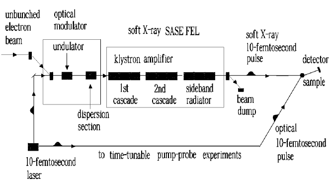
Figure 9: Scheme for time-resolved experiments based on the generation of femtosecond pulses by sideband-seeded soft X-ray cascade klystron amplifier. In this scheme, a femtosecond soft X-ray pulse is naturally synchronized with the femtosecond optical pulse from the seed laser and cancels jitter

Figure 10: Description of the sideband generation for the case of the density modulation as initial condition

Pump-probe techniques which are commonly used with optical lasers, are highly desirable in order to make full use of the femtosecond soft X-ray pulses. Since, in this case, precise timing is needed with a jitter of less than 10 fs, in [19] we suggested to combine the femtosecond soft X-ray pulses generated by the sideband-seeded SASE FEL with optical pulses generated by the seed laser system. It should be emphasized that in the proposed scheme a femtosecond soft X-ray pulse is naturally synchronized with his femtosecond optical pulse and cancels jitter. This development of XFEL based pump-probe experiments allow us to investigate phenomena at timescale down to 100 fs.

7.3 Multi-user distribution system for XFEL laboratory

An X-ray laboratory should serve several, may be up to ten experimental stations which can be operated independently according to the needs of the user community. On the other hand, the multi-user distribution system has to satisfy an additional requirement. Passing the electron bunch through the bending magnets must avoid emittance dilution due to coherent synchrotron radiation (CSR) effects. For very short bunches and very high peak current, CSR can generated energy spread in the bending magnets and thus dilute the horizontal emittance. As a result, the prefered layout of a conventional SASE FEL is a linear arrangement in which the injector , accelerator, bunch compressors and undulators are nearly collinear, and in which the electron beam does not change direction between accelerator and undulators.

The situation is quite different for the klystron amplifier scheme proposed in our paper. Since it operates without bunch compression in the injector linac, the problem of emittance dilution in the bending magnets does not exist. An electron beam distribution system based on unbunched electron beam can provide efficient ways to generate a multi-user facility - very similar to present day synchrotron radiation facilities. A possible layout of a soft X-ray FEL laboratory based on an electron ring distribution system is shown in Fig. 11. The layout of the laboratory follows a similar approach as that used for synchrotron light sources. The SASE FEL user facility consists of an injector linac and electron beam distribution system. The injector is composed of a RF gun with photocathode and a main (superconducting) linac. In order to make efficient use of the new source it is proposed to segment the full circumference of a distribution system into arcs which are repeated a number of times to form a complete ring. Each cell includes a two-cascade klystron and a bending magnet. A specific realization of the electron ring cell is sketched in Fig. 12. The electron beam transport line guiding electrons from the injector linac to the experimental hall is connected tangentially to one of the straight sections of the electron ring. In order to obtain a useful separation between the experimental areas behind the photon beam lines, an angle of 36 degrees between two neighboring lines would be desirable. Thus, ten beam lines can be installed on a complete electron ring. Using klystron (electromagnetic) dispersion sections in each cell as switching elements it is possible to quickly switch the FEL photon beam from one experiment to the other, thus providing multi-user capability. Users can define the radiation wavelength for their experiment independently of each other to a very large extent, since they use different undulators. Injector linac and electron beam transport lines operate at fixed parameters. At a fixed electron energy the magnet gap of the klystron undulators can be varied mechanically for wavelength tuning. This design makes it possible to make various wavelengths of SASE radiation available in the XFEL laboratory quasi-simultaneously. It is a great advantage that injector and electron beam transport lines in the new scheme of multi-user facility operate at fixed parameters and that an ”electron switchard” is not required.

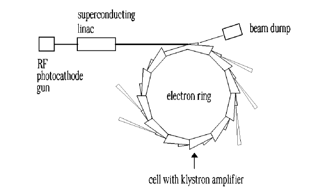
Figure 11: Diagram of a possible fourth-generation synchrotron facility using spontaneous emission free-electron laser klystron amplifiers

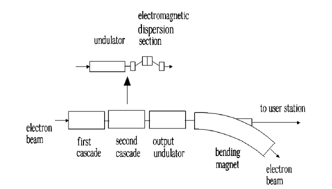
Figure 12: Electron ring cell design. Using a klystron electromagnetic dispersion section as a switching element it is possible to quickly switch off (on) the cell klystron amplifier thus providing multi-user capability. This design makes it possible to make various wavelengths of SASE radiation available in the XFEL laboratory quasi-simultaneously

When a relativistic electron beam passes through the undulator, it emits incoherent radiation. This process leads to an increase of the energy spread in the beam due to quantum fluctuations of the undulator radiation. This effect grows significantly with an increase in electron beam energy, strength field and length of the undulator. This effect should be carefully taken into account when designing multi-user distribution system. For the case of planar undulator the expression for the rate of energy diffusion can be written in the following form[20]:

$$\frac{\mathop{\mathrm{d}}\langle(\Delta\gamma)^{2}\rangle}{\mathop{\mathrm{d}}z}=\frac{7}{15}\frac{\lambda_{\mathrm{c}}}{2\pi}r_{\mathrm{e}}\gamma^{4}k^{3}_{\mathrm{w}}K^{2}F(K)\ ,$$ (64)

where $\lambda_{\mathrm{c}}$ is the Compton wavelength, $r_{\mathrm{e}}$ is the classical electron radius, $F(K)\simeq 1.2K$ for $K\gg 1$. The next numerical example illustrates the amplitude of the effect. If $\gamma=10^{3}$, $K=1.42$, $\lambda_{\mathrm{w}}=3\ {\mathrm{cm}}$, and the total undulator length is equal to 100 m, appropriate substitution in (64) shows that the energy spread increase due to quantum fluctuations is about $\sqrt{\langle(\Delta{\cal E})^{2}\rangle}\simeq 1\ {\mathrm{keV}}$ at the end of the 10th klystron amplifier, and has a negligible effect on the klystron performance.

8 Conclusion

The high-gain klystron amplifier described in this paper is an attractive alternative to other FEL configurations for operation in short wavelength range. An distinguishing feature of the klystron amplifier is the absence of apparent limitations which would prevent operation without bunch compression in the injector linac. We have illustrated the proposed cascade klystron scheme using the parameters of the TESLA Test Facility. Although the present work is concerned primarily for use in the soft X-ray spectrum, its applicability is not restricted to that range, for example an X-ray SASE FEL is a suitable candidate for application of cascade klystron scheme described here.

References

- [1] TESLA Technical Design Report, DESY 2001-011, edited by Richard et al., and http://tesla.desy.de
- [2] The LCLS Design Study Group, LCLS Design Study Report, SLAC reports SLAC-R521, Stanford (1998) and http:www-ssrl.slacstanford.edu/lcls/CDR
- [3] C. Pagani et al., Nucl. Instrum. Methods A 455(2000)733
- [4] J.C. Gallardo, C. Pellegrini, Nucl. Instrum. Methods A 296(1990)448
- [5] V.N. Litvinenko, Nucl. Instrum. Methods A 304(1991)463
- [6] V.A. Bazylev, M.M. Pitatelev, Nucl. Instrum. Methods A 358(1995)64
- [7] G.R. Neil, H.P. Freund, Nucl. Instrum. Methods A 475(2001)381
- [8] N. A. Vinokurov, Nucl. Instrum. Methods A 375(1996)264
- [9] J. Chen, et al., Nucl. Instrum. Methods A 375(1996)299
- [10] Ya. S. Derbenev, A. M. Kondratenko and E. L. Saldin, Nucl. Instrum. Methods 193(1982)415
- [11] V. Ayvazyan et al., Phys. Rev. Lett. 88(2002)194802
- [12] E.L. Saldin, E.A. Scheidmiller, M.V. Yurkov, The physics of Free Electron Lasers, Springer, Berlin-Heiderberg-New York, 1999
- [13] P.L. Czonka, Part. Accel. 8, 225 (1978)
- [14] J. Feldhaus et al., Preprint DESY 03-092, DESY, Hamburg, 2003
- [15] D. A. Bell, Electrical noise, D. Van Nostrand Company, LTD, London, 1960
- [16] R. Bonifacio, L. De Salvo, and Pierini, Nucl. Instrum. Methods A 293(1990)627
- [17] Ciocci, et al., IEEE J. Quantum Electron. 31 (1995)1242
- [18] W. M. Fawley et al., Proceedings of the IEEE 1995 Particle Accelerator Conference, 1996, p.219
- [19] E.L. Saldin, E.A. Scheidmiller, M.V. Yurkov, Optics Commun. 205(2002)385
- [20] E.L. Saldin, E.A. Scheidmiller, M.V. Yurkov, Nucl. Instrum. Methods A 381(1996)545