Foreign exchange market fluctuations as random walk in demarcated complex plane

Abstract

We show that time-dependent fluctuations $\{\Delta x\}$ in foreign exchange rates are accurately described by a random walk in a complex plane that is demarcated into the gain ($+$) and loss ($-$) sectors. $\Delta x$ is the outcome of $N$ random steps from the origin and $|\Delta x|$ is the square of the Euclidean distance of the final $N$-th step position. Sign of $\Delta x(t)$ is set by the $N$-th step location in the plane. The model explains not only the exponential statistics of the probability density of $\{\Delta x\}$ for G7 markets but also its observed asymmetry, and power-law dependent broadening with increasing time delay.

Easier data access via the Internet and the widespread availability of powerful computers, have enabled many researchers not just in business and economics Lipton (2001) but also in physics, applied mathematics, and engineering Ghashghaie et al. (1996); Mantegna and Stanley (1996); Friedrich et al. (2000); Buchanan (2002), to investigate more deeply the dynamics of foreign exchange markets. Their efforts have led to new insights on the characteristics of forex rate fluctuations including the general behavior of their corresponding probability density function (pdf) Ghashghaie et al. (1996); Friedrich et al. (2000).

Arguably, forex markets have a more immediate and direct impact on citizens than stock markets do. This is especially true in developing countries where only a minority holds stocks directly while a majority sells or purchases products and commodities on a daily basis. Economies that rely strongly on remittances of overseas contract workers (e.g. Philippines) or tourism (e.g. Thailand), are also quite sensitive to forex rate instabilities. Hence, knowledge of the vagaries of the forex market, is important not only to policymakers and macroeconomic managers in government and banking sectors but also to individual businessmen and consumers.

The exchange rate of a currency relative to another (usually the US dollar) is represented by a time-series of quotations $\{x(t)\}$, where time $t=m\Delta t$, $\Delta t=$ time delay, and index $m=1,2,\ldots,M$. Normally, the power spectrum of $\{x(t)\}$ consists of one or two dominant low-frequency components and a continuous high-frequency band. The low-frequency components reveal the longterm behavior of $\{x(t)\}$ and therefore the soundness of a national economy from the perspective of economic fundamentals. The high-frequency components are associated with fluctuations in $\{x(t)\}$ that arise from complex interactions between market players over short time-scales ($\Delta t<2$ days) Ghashghaie et al. (1996); Friedrich et al. (2000).

The statistics of the (percentage) rate fluctuations $\{\Delta x(t)\}=\{\Delta x\}$ in G7 markets is described by an exponentially-decaying pdf $p(\Delta x,\Delta t)$ where: $\Delta x(t)=[x(t+\Delta t)-x(t)][100/x(t)]$. This statistical behavior is not easily seen from the power spectrum of $\{x(t)\}$. Figure 1 shows the $p(\Delta x,\Delta t)$’s for the Japanese (1a) and Philippine (1b) markets. For the G7 Federal Reserve Board (2002) and Philippine Bangko Sentral ng Pilipinas markets, our core data sets for $\{x(t)\}$ comprise of daily closing rates from January 1971 to December 1993 ($M=5000$ trading days, $\Delta t=1$ day). The Philippine market was under exchange control in the 70’s and its $p(\Delta x,\Delta t)$ has a large number of points around $\Delta x=0$.

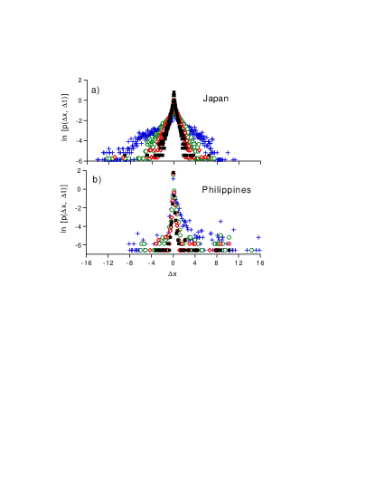
Figure 1: Asymmetric $p(\Delta x,\Delta t)$’s: a) Japan, and b) Philippines for $\Delta t$ (day) $=1$ (filled squares), $2$ (diamonds), $5$ (circles), and $20$ (cross-hairs). For any $\Delta t$, $p(\Delta x,\Delta t)$ is normalized i.e., $\sum p(\Delta x,\Delta t)\delta x=1$, where histogram bin-width $\delta x=(2/201)[{\rm max}(\Delta x_{\rm max},|-\Delta x_{\rm min}|)]$. Summation is for all $\Delta x$’s.

Most $p(\Delta x,\Delta t)$’s exhibit a degree of asymmetry about $\Delta x=0$. An asymmetric $p(\Delta x,\Delta t)$ is described by a pair of exponents $\alpha_{l}$ and $\alpha_{r}$ for $\Delta x<0$ (left) and $\Delta x>0$ (right), respectively. It is displayed by currencies that have either appreciated (e.g. Japan) or depreciated (e.g. Canada, Philippines) against the USD during the sampling period.

Table 1 lists the best-fit values (by least-squares method) of $\alpha_{l}$, $\alpha_{r}$ and the left and right intercepts $\beta_{l}$ and $\beta_{r}$ of $p(\Delta x,\Delta t=1\;{\rm day})$ with the $\Delta x=0$ line for the G7 markets. The exponential behavior of $p(\Delta x,\Delta t)$ persists even for $\Delta t$’s $>2$ days. We also found that $p(\Delta x,\Delta t)$ broadens with $\Delta t$ in a power-law trend.

Table 1: Parameter values of exponential fit: $\beta\exp(\alpha\Delta x)$, to $p(\Delta x,1$ day$)$ for G7 and Philippine markets. For a symmetric $p(\Delta x,\Delta t)$: $\alpha_{l}=|\alpha_{r}|$, and $\ln(\beta_{l})=\ln(|\beta_{r}|)$.

Country	$\alpha_{l}$	$\alpha_{r}$	$\ln(\beta_{l})$	$\ln(\beta_{r})$
Canada	$6.143\pm 0.197$	$-5.807\pm 0.150$	$1.090\pm 0.071$	$1.037\pm 0.058$
France	$2.283\pm 0.082$	$-2.469\pm 0.096$	$0.056\pm 0.065$	$0.181\pm 0.069$
Germany	$2.166\pm 0.076$	$-2.327\pm 0.068$	$0.058\pm 0.062$	$0.125\pm 0.050$
Italy	$2.316\pm 0.113$	$-2.44\pm 0.102$	$-0.012\pm 0.090$	$0.152\pm 0.074$
Japan	$2.371\pm 0.115$	$-2.635\pm 0.084$	$0.073\pm 0.092$	$0.187\pm 0.062$
UK	$2.171\pm 0.091$	$-2.244\pm 0.086$	$0.004\pm 0.074$	$0.063\pm 0.066$
Philippines	$4.711\pm 0.904$	$-2.892\pm 1.063$	$-1.745\pm 0.564$	$-1.464\pm 0.964$

The behavior of $\{x(t)\}$ has been described previously as a Markov process with multiplicative noise and the emergence of a highly-symmetric $p(\Delta x,\Delta t)$ such as that of the German market Ghashghaie et al. (1996); Friedrich et al. (2000), is explained by the Fokker-Planck equation. However, these studies did not explain the emergence of asymmetric $p(\Delta x,\Delta t)$’s and the power-law behavior of their broadening with $\Delta t$.

Here, we show that the statistics of $\{\Delta x\}$ is accurately described by a random walk on a demarcated complex plane. Our model accounts for possible asymmetry of $p(\Delta x,\Delta t)$, its broadening with increasing $\Delta t$, and the power-law behavior of this broadening for G7 markets. Each $\Delta x$ is the outcome of $N$ random steps that start from the plane origin O (see Fig 2). Its magnitude is $|\Delta x|=d^{2}$, where $d$ is the Euclidean distance of the $N$-th step endpoint N($x_{R},x_{I}$) from origin O, and $x_{R}$ and $x_{I}$ are the real and imaginary coordinates. The sign of $\Delta x$ depends on the location of N($x_{R},x_{I}$) in the plane which is demarcated by the polar angle $\Theta$, into two regions representing the gain ($+$) and loss ($-$) regimes.

\psfrag{Q}{$\Theta$}\psfrag{Q=0}{$\Theta=0$}\includegraphics[width=216.81pt]{Fig2}

Figure 2: Random walk in complex plane demarcated by angle $\Theta$, into gain ($+$) and loss ($-$, shaded) regions. Each $\Delta x$ is the outcome of N random steps from origin O where: $d=\left(x_{R}^{2}+x_{I}^{2}\right)^{1/2}$, and $|\Delta x|=d^{2}$. Sign of $\Delta x$ is given by location of endpoint N($x_{R}$, $x_{I}$) in the plane. The n-th phasor is the fluctuation $|\Delta x_{n}|=|a_{n}|^{2}$, of the $n$-th dealer where $n=1,2,,N$.

Random walk in complex plane. The location of N($x_{R},x_{I}$) is given by the sum of $N$ elementary phasors $\{a_{n}\}$ Goodman (1984); Woods and Stark (2001): ${\rm N}(x_{R},x_{I})=\sum_{n=1}^{N}\;a_{n}(x_{R},x_{I})=\sum_{n=1}^{N}\;|a_{n}|\exp(j\;\theta_{n})$ where $j=(-1)^{1/2}$. The amplitude $|a_{n}|$ and phase $\theta_{n}$ of the $n$-th phasor are statistically independent of each other and of the amplitudes and phases of all other ($N-1$) $a_{n}$’s. Possible $|a_{n}|$ values are uniformly distributed within a predetermined (non-negative) range. Phases $\theta_{n}$ are also uniformly distributed: $0\leq\theta_{n}\leq 2\pi$.

Consistent with the central-limit theorem, the location of N($x_{R},x_{I}$) is governed by a Gaussian pdf ($N\rightarrow\infty$) Goodman (1984): $p_{N}(x_{R},x_{I})=(2\pi\sigma^{2})^{-1}\;\exp[-(x_{R}^{2}+x_{I}^{2})/2\sigma^{2}]$, where $\sigma^{2}$ is the variance. Hence, the $d^{2}$-values obey a negative-exponential statistics: $p_{d}(d^{2})=(2\sigma^{2})^{-1}\exp(-d^{2}/2\sigma^{2})$. The $q$-th moment $\langle(d^{2})^{q}\rangle$ of $d^{2}$ is given by: $\langle(d^{2})^{q}\rangle=q!(2\sigma^{2})q=q!\langle d^{2}\rangle^{q}$, where the mean value $\langle d^{2}\rangle$ is $2\sigma^{2}$. Phase $\theta$ of N($x_{R},x_{I}$) obeys a uniform statistics: $p_{\theta}(\theta)=(2\pi)^{-1}$ for $-\pi\leq\theta\leq\pi$; $p_{\theta}(\theta)=0$, otherwise.

The joint (second-order) pdf of $d_{1}^{2}$ and $d_{2}^{2}$ at two different time instants is Goodman (1984): $p_{d}(d_{1}^{2},d_{2}^{2})=$ $\left[\langle d^{2}\rangle^{2}(1-|\mu|^{2})\right]^{-1}\exp\left\{-\left(d_{1}^{2}+d_{2}^{2}\right)/\left[\langle d^{2}\rangle(1-|\mu|^{2})\right]\right\}$ $J_{0}\left\{2d_{1}d_{2}|\mu|/\left[\langle d^{2}\rangle(1-|\mu|^{2})\right]\right\}$, where: $\langle d_{1}^{2}\rangle=\langle d_{2}^{2}\rangle=\langle d^{2}\rangle$, $J_{0}(x)$ is the zero-order Bessel function of the first kind, and $|\mu|$ is the modulus of a complex factor that measures the degree of correlation between events at two different time-instants. If $|\mu|=0$ (no correlation), $p_{d}(d_{1}^{2},d_{2}^{2})=p_{d}(d_{1}^{2})\;p_{d}(d_{2}^{2})$. On the other hand, $p_{d}(d_{1}^{2},d_{2}^{2})=p_{d}(d_{1}^{2})\;\delta(d_{1}^{2}-d_{2}^{2})$, as $|\mu|\rightarrow 1$, where $\delta(x)$ is the Dirac delta function.

As it is, the statistics of a random walk in a complex plane is insufficient to describe the characteristics of the $p(\Delta x,\Delta t)$’s of forex markets because the possible $\Delta x$’s are from $-\infty$ to $\infty$, while $d^{2}\geq 0$.

Demarcated complex plane. We solve the problem by demarcating the complex plane into two sectors representing the gain ($+\Delta x$) and loss ($-\Delta x$) regimes, where we identify that: $|\Delta x|=d^{2}$. The gain area is set by the polar angle $\Theta$ (counterclockwise rotation) and $\Delta x$ is positive (negative) if N($x_{R},x_{I}$) is on the gain (loss) sector. The gain (loss) area is zero if $\Theta=0$ ($\Theta=2\pi$).

Figure 3 presents exponentially-decaying histograms of $\Delta x$’s generated at $\Theta=0$, $\pi/2$, $\pi$, $3\pi/2$, and $2\pi$ (360 deg). The histograms are asymmetric about $\Delta x=0$ at all angles except at $\Theta=\pi$ where the plane is equally divided between the gain and loss sectors. The corresponding $\Theta$’s for the G7 markets in Table 1 are not easily determined since $\Theta$ is not clearly related with $\alpha_{l}$, $\alpha_{r}$, $\beta_{l}$, and $\beta_{r}$. However, our model reveals a unique relation between $R=A_{l}/A_{r}$ and $\Theta$, where $A_{l}$ ($A_{r}$) is the area under the best-fit exponential for $\Delta x<0$ ($\Delta x>0$) of the histogram.

Figure 3: Random walk in demarcated complex plane. Histograms of $\Delta x$ s for $\Theta=0$ (squares), $\pi/2$ (diamonds), $\pi$ (circles), $3\pi/2$ (triangles) and $2\pi$ (crosses) where N $=50$, $0\leq|a_{n}|\leq 0.015$ (double precision).

Figures 4a-b plot the average $\langle R\rangle$ as a function $N$ and number of trials, respectively ($\Theta=\pi$). $\langle R\rangle$ is insensitive to $N$ but for a fixed $N$, the standard deviation of $\langle R\rangle$ decreases quickly (power-law decay) with the number of trials . Figure 4c shows that the dependence of $\langle R\rangle$ with $\Theta$ is well-described by: $\langle R\rangle=\Theta/(360\;{\rm deg}-\Theta)$.

Figure 4: $\langle R\rangle$ as a function of ($\Theta=\pi$): a) $N$, b) Number of trials per datapoint ($N=50$) ($\langle$s.d.$\rangle$ $=1.05$.), and c) $\Theta$ for $N=50$. $10$ trials for each datapoint.

The $\langle R\rangle$’s are calculated from $p(\Delta x,\Delta t)$’s of the G7 markets and then used to determine their corresponding $\Theta$’s via the $R(\Theta)$-curve. The following $\Theta$’s (deg) were obtained ($\Delta t=1$ day): Canada ($179.7$), France ($180.4$), Germany ($182.3$), Italy ($177.8$), Japan ($177.6$), and UK ($174.9$). For the G7 markets, differences in the size of the gain and loss sectors are small ($<4\%$). On the other hand, the $p(\Delta x,1\;{\rm day})$ for the Philippine market is highly asymmetric with a significantly small gain region ($\Theta=108.1$ deg). Against the USD, the Philippine peso depreciated by $246\%$ from December 1983 (lifting of exchange control) to December 1993.

Broadening of $p(\Delta x,\Delta t)$ with time delay $\Delta t$. For the G7 markets, $p(\Delta x,\Delta t)$ broadens with increasing $\Delta t$, while preserving its original negative exponential statistics within: $1\leq\Delta t\;({\rm day})\leq 20$. Previous studies on broadening were confined to $\Delta t<12$ hours Friedrich et al. (2000).

Figure 5 plots the dependence of $\alpha_{l}$ and $\alpha_{r}$ with $\Delta t$ for the G7 markets where a power-law behavior is observed. Except for Canada, the dependence of $\alpha_{l}$’s (and $|\alpha_{r}|$’s) is remarkably described by one and the same power-decay curve (Reference curve 2) indicating a scale-free behavior for the market dynamics. For the Philippine market, the $\Delta t$-dependence of the $\alpha_{l}$ ($\alpha_{r}$)-values is erratic with large standard deviations – there is increasing asymmetry for $p(\Delta x,\Delta t)$ with $\Delta t$. Exchange control destroyed the scale-free behavior of the Philippine market. The largest standard deviation for Canada and UK is $\pm 0.2$ and $\pm 0.1$, respectively which happens at $\Delta t=1$ day, while for Philippines it is $\pm 1.4$ ($\Delta t=3$ days). For any G7 market, $\langle\Delta x\rangle$ increases with $\Delta t$ according to a power law since the exponent is inversely proportional to $1/2\sigma^{2}=1/\langle\Delta x\rangle$.

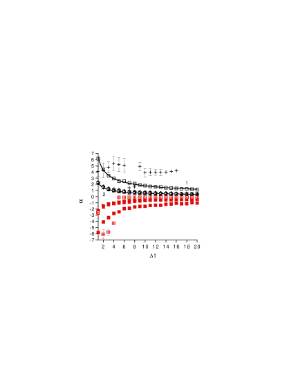
Figure 5: Dependence of $\alpha_{l}$ (positive) and $\alpha_{r}$ (negative) with $\Delta t$ for Canada (squares for $\alpha_{l}$, solid squares for $\alpha_{r}$), France (right triangles), Germany (inverted triangles), Italy (diamonds), Japan (triangles), UK (circles) and Philippines (crosses for $|\alpha_{l}|$, crossed squares for $\alpha_{r}$). Reference curves: $\alpha_{l}=6.4\Delta t-0.561$ (Curve 1) and $\alpha_{l}=2.21\Delta t-0.593$ (Curve 2). $p(\Delta x_{Q},Q)$ contains $5000$ datapoints and each point is the average of $10$ trials.

The observed power-law dependence of the broadening of $p(\Delta x,\Delta t)$ with $\Delta t$ is explained as follows. Let $\langle\Delta x_{Q}\rangle=\langle d_{T}\rangle^{2}$, be the average fluctuation corresponding to a longer time-delay $\Delta t_{Q}=Q\Delta t$, where: $d_{T}=|\sum_{q}d_{q}\exp(j\theta_{q})|$ $=[(\sum_{q}d_{q}\cos\theta_{q})^{2}+(\sum_{q}d_{q}\sin\theta_{q})^{2}]^{1/2}$, $\Delta t$ is the basic time delay, and $q=1,2,\ldots,Q$. If $\langle d_{1}\rangle=\langle d_{2}\rangle=\ldots=\langle d_{Q}\rangle$, then $\langle d_{T}\rangle=\langle d_{1}\rangle\langle[(\sum_{q}\cos\theta_{q})^{2}+(\sum_{q}\sin\theta_{q})^{2}]^{1/2}\rangle\approx Q^{p}\langle d_{1}\rangle$.

The $\langle d_{T}\rangle$ value depends on the probability distribution of $\{\theta_{q}\}$. If the $\theta_{q}$’s are statistically independent and uniformly distributed within $[0,2\pi]$ then $d_{T}\approx Q^{1/2}\langle d_{1}\rangle$, i.e. $p\approx 0.5$. Figure 6 inset plots $\alpha_{l}$ and $|\alpha_{r}|$ of $p(\Delta x_{Q},Q)$ with $Q$ for the above case which verifies our assumption of a power-law dependence of $\langle d_{T}\rangle$ with $\langle d_{1}\rangle$.

Figure 6 plots $p$ as a function of uncertainty spread $\delta\theta$. If $\theta_{q}$’s are restricted such that $\theta_{q+1}$ ($q>1$) is uniformly-random within the forward ($-\pi/2\leq\theta_{q}-0.5\delta\theta\leq\theta_{q+1}\leq\theta_{q}+0.5\delta\theta\leq\pi/2$) and opposite ($\pi/2\leq(\theta_{q}+\pi)-0.5\delta\theta\leq\theta_{q+1}\leq(\theta_{q}+\pi)+0.5\delta\theta\leq 3\pi/2$) directions then: $0\leq p\leq 0.5$. If the $\theta_{q}$’s occur only within the forward or opposite direction then $0.5\leq p\leq 1$. In all cases, $\theta_{1}$ is uniformly-random in the range $[0,2\pi]$.

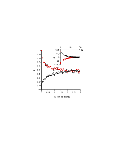
Figure 6: Power $p$ vs. $\delta\theta$. Possible directions of $\Theta_{q}$’s are always forward or always backward (filled circles). Each datapoint is average of $10$ trials. Reference curve: $p=(\delta\theta)^{0.24}$. Inset: $\alpha_{l}$ and $\alpha_{r}$ of $\ln[p(\Delta x_{Q},Q)]$ vs $Q$ for $Q$ (deg) $=90$ (squares), $180$ (circles), and $270$ (diamonds). Reference curve: $\alpha_{l}=76.6Q^{-1}$.

A G7 market exhibits a $(\Delta t)^{-0.5}$-dependence (i.e. $p\approx 1/4$) of $\alpha_{l}$ (Fig 5) because $d_{q+1}$ is equally likely to be in the same or opposite direction of $d_{q}$, with $\delta\theta\approx 0.3$ (17 deg). For a market where the directions of $d_{q+1}$ and $d_{q}$ are statistically independent of each other, the decay of $\alpha_{l}$ with $\Delta t$ is faster ($p\approx 1/2$, Fig 6 inset).

In our model, the forex market consists of $N$ independent players where $\Delta x$ is treated as a random walk of $N$ steps in the demarcated complex plane where $|a_{n}|^{2}$ represents the fluctuation $|\Delta x_{n}|$ of the $n$-th player. Plane anisotropy leads to asymmetric $p_{d}(d^{2})$’s. Our model also explains the power-law dependent broadening of the $p(\Delta x,\Delta t)$’s with $\Delta t$ in G7 markets.

$\Delta x$ is interpreted as the intensity of the resultant complex amplitude that arises from the linear superposition of the fluctuations of the $N$ independent dealers. Interactions between players arises inherently because the intensity which is the product of the resultant complex amplitude and its conjugate, contains interference terms between the contributions of the individual players. We showed that real market dynamics could be analyzed accurately with a relatively low number of the interacting players. The interaction between the multitude of agents in a real market could be effectively reduced into one with a low number of representative classes.

Our model currently neglects the phenomenon of allelomimesis which causes social agents to clusterJuanico et al. (2003). Herding (bandwagoning) among market dealers could trigger massive selling or buying in financial markets and leads to large swings in $\{x(t)\}$ like those found in the middle 1980’s for the G7 markets. The same limitation is found in previous models of forex markets Mantegna and Stanley (1996); Friedrich et al. (2000).

Acknowledgement. J Garcia for stimulating discussions and assistance in data acquisition (Philippine peso).

References

- Lipton (2001) A. Lipton, Mathematical Methods For Foreign Exchange: A Financial Engineer’s Approach (World Scientific, New York, 2001); R. Gencay, G. Ballocchi, M. Dacorogna, R. Olsen, and O. Pictet, Int Economic Rev 43, 463 (2002); J. Danielsson and R. Payne, J Int Money Finance 21, 203 222 (2002); I. Moosa and J. Post, Keynesian Economics 24, 443 (2002).
- Ghashghaie et al. (1996) S. Ghashghaie, W. Breymann, J. Peinke, P. Talkner, and Y. Dodge, Nature (London) 381, 767 (1996).
- Mantegna and Stanley (1996) R. Mantegna and H. Stanley, Nature (London) 383, 587 (1996).
- Friedrich et al. (2000) R. Friedrich, J. Peinke, and C. Renner, Phys Rev Lett 84, 5224 (2000); M. Karth and J. Peinke, Complexity 8, 34 (2002).
- Buchanan (2002) M. Buchanan, Nature (London) 415, 10 (2002); L. Matassini, Physica A 308, 402 (2002); K. Izumi and K. Ueda, IEEE Trans Evolutionary Computation 5, 456 470 (2001); H. White and J. Racine, IEEE Trans Neural Networks 12, 657 (2001); J. Yao and C. Tan, Neurocomputing 34, 79 98 (2000); A. Nag and A. Mitra, J Forecasting 21, 501 511 (2002).
- Federal Reserve Board (2002) Federal Reserve Board, Statistics: Releases and Historical Data, http//www.federalreserve.gov/releases/ (2002).
- (7) Bangko Sentral ng Pilipinas, Exchange Rates of the Philippine Peso, Selected Economic and Financial Indicators (SEFI), http://www.bsp.gov.ph.
- Goodman (1984) J. Goodman, Statistical Properties of Laser Speckle Patterns in Topics in Applied Physics: Laser Speckle and Related Phenomena, JC Dainty, ed. (Springer-Verlag, New York, 1984).
- Woods and Stark (2001) J. Woods and H. Stark, Probability and Random Processes with Applications to Signal Processing (Prentice Hall, New York, 2001), 3rd ed.
- Juanico et al. (2003) D. Juanico, C. Monterola, and C. Saloma, Physica A 320C, 590 (2003).