On Statistical Methods of Parameter Estimation
for Deterministically Chaotic Time-Series

Abstract

We discuss the possibility of applying some standard statistical methods (the least square method, the maximum likelihood method, the method of statistical moments for estimation of parameters) to deterministically chaotic low-dimensional dynamic system (the logistic map) containing an observational noise. A “pure” Maximum Likelihood (ML) method is suggested to estimate the structural parameter of the logistic map along with the initial value $x_{1}$ considered as an additional unknown parameter. Comparisons with previously proposed techniques on simulated numerical examples give favorable results (at least, for the investigated combinations of sample size $N$ and noise level). Besides, unlike some suggested techniques, our method does not require the a priori knowledge of the noise variance. We also clarify the nature of the inherent difficulties in the statistical analysis of deterministically chaotic time series and the status of previously proposed Bayesian approaches. We note the trade-off between the need of using a large number of data points in the ML analysis to decrease the bias (to guarantee consistency of the estimation) and the unstable nature of dynamical trajectories with exponentially fast loss of memory of the initial condition. The method of statistical moments for the estimation of the parameter of the logistic map is discussed. This method seems to be the unique method whose consistency for deterministically chaotic time series is proved so far theoretically (not only numerically).

The problem of characterizing and quantifying a noisy nonlinear dynamical chaotic system from a finite realization of a time series of measurements is full of difficulties. The first one is that one rarely has the luxury of knowing the underlying dynamics, i.e., one does not in general know the underlying equations of evolution. Techniques to reconstruct a parametric representation of the time series then may lead to so-called model errors.

Even in the rare situations where one can ascertain that the measurements correspond to a known set of equations with additive noise, the chaotic nature of the dynamics makes the estimation of the model parameters from time series surprisingly difficult. This is true even for low-dimensional systems, another even rarer instance in naturally occurring time series.

Here, we revisit the problem proposed by McSharry and Smith McSharrySmith , who introduced an improved method over standard least-square fits to estimate the structural parameter of a low-dimensional deterministically chaotic system (the logistic map). We discuss the caveats underlying this problem, propose a “pure” Maximum Likelihood method that we compare with previously proposed methods. Our conclusion stresses the inherent difficulties in formulating a bona fide statistical theory of structural parameter estimations for noisy deterministic chaos.

I Definition and nature of the problem

Let us consider the supposedly simple problem considered by McSharry and Smith McSharrySmith , in which one measures the sample $s_{1},...,s_{N}$ with

$$s_{i}=x_{i}+\eta_{i}$$ (1)

where the underlying dynamical one-dimensional discrete recurrence equation

$$x_{i+1}=F(x_{i},a)\equiv 1-ax_{i}^{2}~{}$$ (2)

is known and the $\eta_{i}$’s are Gaussian $N(0,\epsilon)$ iid random variables with zero mean and standard deviation $\epsilon$. The problem is to determine the model parameter $a$ from the measurements $s_{1},...,s_{N}$, knowing that (2) is the true dynamics.

At first sight, this problem looks like a statistical estimation of an unknown structural parameter, given observational data. However, strictly speaking, this problem cannot be (even formally) refered to as a bona fide statistical problem in which the maximum likelihood (ML) method can be proved to be asymptotically optimal or even consistent. Indeed, the Likelihood Function $L(a,x_{1}|s_{1},...,s_{N})$ reads

$$\ln L(a,x_{1}|s_{1},...,s_{N})\propto-N\ln(\epsilon)-{1\over 2\epsilon^{2}}\sum_{i}\left(s_{i}-F^{(i)}(x_{1},a)\right)^{2}~{},$$ (3)

where $F^{(i)}(x_{1},a)$ is the $i$-th iteration of the logistic map (2) with parameter $a$ and initial value $x_{1}$. The key point of difficulty is that $F^{(i)}(x_{1},a)$ is a non-stationary function (despite the fact that the dynamical system (2) has an invariant measure $\mu(x)$). Standard statistical ML methods are applicable either to functions not depending on $i$, or depending on $i$ in a periodic manner. For non-stationary and non-periodic dependence of the function on $i$, no statistical theorem on optimal properties of MLE is a priori applicable. Then, numerical simulations of examples are not enough and should be complemented with proofs of results stating what known mathematical statistics properties of ML or of Bayesian methods continue to apply to (3). A first taste of the difficulty of the problem is given by an analysis of the behavior of the “one-step least-square (LS) estimation” and of the “total least-square” method, given in Appendix A. Appendix A shows that least-square methods are biased and should be corrected before comparing these to other methods, as done in McSharrySmith . In particular, Appendix A shows that it was a priori unfair or inappropriate to compare any estimate obtained with a given method (such as the one advocated by McSharry and Smith McSharrySmith ) to uncorrected ML-estimates due to the non-stationarity of the function; the appropriate corrections can be obtained from the standard statistical theory of confluence analysis FrischR ; Geary ; KendallStuart .

II A “pure” Maximum Likelihood approach in terms of $(a,x_{1})$

Putting aside the question of a rigorous demonstration of the consistency and asymptotic optimality of the MLE method, let us come back to expression (3), which is the straightforward translation of the iid Gaussian $N(0,\epsilon)$ properties of the random variables $\eta_{i}$’s. It suggests that the problem of estimating the structural parameter $a$ cannot actually be separated from estimating simultaneously the initial value $x_{1}$.

The MLE of $(a,x_{1})$ amounts in this case to the minimization of the sum:

$$\sum_{i}\left(s_{i}-F^{(i)}(x_{1},a)\right)^{2}~{},$$ (4)

which looks superficially as a standard non-linear least-square sum. There is however one very important distinction, as we already pointed out above: the non-linear function depends on the index $i$ whereas, in the standard least-square method, one has a sum of the type

$$\sum_{i}\left(s_{i}-F(x_{i},a)\right)^{2}~{},$$ (5)

where the $x_{1},...,x_{N}$ are assumed to be known.

For the parameters $a$ for which the logistic map exhibits the phenomenon of sensitivity upon the initial condition, the direct minimization of (4) is not feasible directly. Indeed, if we disturb $x_{1}$ by a small number $\delta$, then the $i$th iterations $F^{(i)}(x_{1},a)$ and $F^{(i)}(x_{1}+\delta,a)$ diverge asymptotically exponentially fast with $i$: for instance, with an accuracy $\delta=10^{-15}$ and for $a=1.85$, the difference $F^{(i)}(x_{1},a)-F^{(i)}(x_{1}+\delta,a)$ becomes of order $1$ for $i>20$. This implies that, in practice, we cannot calculate with the necessary accuracy $x_{i+1}=F^{(i)}(x_{1},a)$ for $i>20$. To address this fundamental limitation, we propose to cut the sample $s_{1},...,s_{N}$ into $n_{1}$ portions of size no more than $n_{2}=20$, and to treat each portion separately. This amounts to re-estimating a different initial condition for each such sub-series, which is a natural step since the sensitivity upon initial conditions amounts to losing the information on the specific value of the initial condition.

Our numerical tests show that our MLE works well (see below) by considering sub-series of size in the range $n_{2}=4-25$ (for the true value of $a$ equal to the value $1.85$ considered by by McSharry and Smith McSharrySmith that we take as our benchmark for the sake of comparison). For larger samples (say, $N=100$), we recommend to cut this sample into $n_{1}$ subsamples of size $n_{2}=4-25$, and treat them separately. It is possible that we lose some efficiency in treating subsamples separately, but a joint estimation would require the maximization of the likelihood with the common parameter $a$ and several different initial value parameters. This procedure would lead to a very difficult numerical multivariate search problem as any gradient method would fail due to the very irregular structure of the likelihood function (see below and figure 1).

The procedure we propose is thus to cut the initial time-series into $n_{1}$ independent subsamples of size $n_{2}$ in the range $4-25$, and to average the resulting $n_{1}$ $a$-estimates. In order to determine the optimal value of $n_{1}$ for a fixed $N$ (say $N=100$) and for the value $a=1.85$ investigated here, we calculate the standard deviation sdt$(a)$ over the $n_{1}$ subsamples as a function of $n_{1}$. We find that, basically independently of the noise level $\epsilon$, the pair $n_{1}=25,n_{2}=4$ gives the smallest standard deviation sdt$(a)$.

We have implemented this approach and compared it with the results obtained by the method proposed by McSharry and Smith McSharrySmith , as discussed in the next section.

III ML version of McSharry and Smith McSharrySmith and comparisons

The main result of McSharry and Smith’s paper McSharrySmith consists in their formulae (13,14) for their proposed ML cost function. Their idea is to substitute in the ML cost function the unknown invariant measure $\mu_{a}(x)$ of the dynamical system (2), for a given value of the parameter $a$, for what should be a realization of the latent variables $x_{i}$’s. Notice that $a$ should be varied in order to determine the maximum likelihood. In practice, the integral over the unknown invariant measure $\mu_{a}(x)$ is replaced by a sum over a model trajectory (which can be calculated since the model is assumed to be known) of length $\tau\gg N$. Unfortunately, this most important step is not confirmed by any numerical results (see below).

Before continuing, let us note that there is a mistake in the probability density function (pdf) and likelihood given by their equations (7-9). Using the intuition that pairs $(s_{i},s_{i+1})$ should be used in their equation (5, 6) to track the deterministic relation between $x_{i}$ and $x_{i+1}=F(x_{i},a)$, we see that a single latent variable $x_{i}$ is associated with each pair $(s_{i},s_{i+1})$ since $s_{i}$ is compared with $x_{i}$ and $s_{i+1}$ with $F(x_{i},a)$. Thus, each $x_{i}$ is used only once when scanning all possible pairs $(s_{i},s_{i+1})$, for $i=1,...,N-1$ and in their ML cost function (13,14). Actually, the correct likelihood should use only once each observed random variable $s_{i}$, not the latent variable $x_{i}$. Therefore, using pairs $(s_{i},s_{i+1})$, McSharry and Smith take into account each $s_{i},i=2,...,N-1$ twice, and the end values $s_{1},s_{N}$ once. For $N\gg 2$, their expression (7) is approximately equals (up to the end terms) to the square of the correct likelihood. Taking the logarithm in their equation (13) gives approximately twice the correct likelihood, which gives almost the same estimate as the exact likelihood.

While this mistake has no serious consequences for the numerical accuracy of their calculation for long time series $N\gg 2$, it illustrates the difference between their construction of the likelihood and our direct approach presented in the previous section. By writing the conditional likelihood for a pair $(s_{i},s_{i+1})$ under a latent variable $x_{i}$, and by averaging this conditional likelihood weighted by the invariant measure $\mu(x|a)$, McSharry and Smith suggest that, by doing so, they incorporate additional information on the system in question. If we had a usual probability space, then such averaging would provide the unconditional likelihood of the pair $(s_{i},s_{i+1})$ but, for deterministically chaotic time series, the exact meaning of this averaging is not clear. Another questionable step of McSharry and Smith is to multiply these pairwise likelihoods as if the pairs $(s_{i},s_{i+1})$ were independent. If this was so, this would indeed give the unconditional likelihood for the data sample $s_{1},...,s_{N}$.

But, we deal here with “deterministic chaos” which generates not truly random variables (see for instance SorArn ; Phatak for discussions on the pseudo-randomness nature of such time series). Besides, we have some more information about the structure of the system in question. Namely, we suppose known the generating relation (2). This relation contains everything and is, in principle, much more informative than the stationary invariant measure $\mu(x|a)$ (which is akin to a one-point statistics while (2) contains information on all higher-order point statistics). Concretely, it is clear that the product of pdf’s for each pair $(s_{i},s_{i+1})$ and the resulting likelihood depends solely on the first initial value $x_{1}$ since all subsequent $x_{i}$ are deterministically determined recurrently. This remark gives the likelihood function (3) in terms of two unknown parameters $(a,x_{1})$ to be estimated. This leads indeed to consider the initial state variable $x_{1}$ as an unknown parameter to be estimated (along with $a$) from the sample $s_{1},...,s_{N}$. The likelihood (3) provides a more detailed form than obtained by averaging over the invariant measure $\mu(x|a)$. We can hope that our approach would lead to a more efficient estimate of $a$. McSharry and Smith avoid the maximization with respect to $x_{1}$ in their likelihood (13,14) and replace it by an averaging over a proxy of the invariant measure. It is doubtful that such a step is warranted, not speaking of optimality, in view of our numerical tests presented below.

We now compare our “pure” Maximum Likelihood approach in terms of $(a,x_{1})$ proposed in section II with McSharry and Smith’s ML method, using numerical tests. We consider 1000 time series with $N=100$ data points and subdivide each of them into $n_{1}=25$ sub-series of $n_{2}=4$ data points. We fix the true $a$ equal to $1.85$ as in McSharrySmith and study noises with standard deviations equal to $0.5$ and $1.0$. Table 1 shows a significant improvement offered by our “pure” ML method over McSharry and Smith’s average ML, as least for the set of parameters studied here. It is not possible to guarantee that this will be the case for all possible parameter values but we believe our method can not be worse that McSharry and Smith’s average ML. A difficulty that should be mentioned is that the chaotic nature of the dynamics and in particular the sensitivity of the invariant measure with respect to the control parameter $a$ is reflected into an ugly-looking log-Likelihood landscape shown in Figure 1, with many competing valleys. Standard numerical methods like gradient or simplex are unapplicable. We have used a systematic 2D-grid search. Other methods in the field of computational intelligence, such as stimulated annealing and genetic algorithms, could also be used. The sensitivity of the invariant measure with respect to the control parameter $a$ means that the invariant distribution can bifurcate from an almost uniform distribution on the interval $[-a,1]$ to a distribution consisting of three delta-functions (this happens around $a\approx 1.75$).

noise		mean$(a)$	std$(a)$	$q_{1}$	$q_{2}$	$q_{2}-q_{1}$	${\hat{\epsilon}}$
std $0.5$	Ref.McSharrySmith	$1.816$	$0.0714$	$1.630$	$1.925$	$0.295$
	“pure” ML	$1.841$	$0.0390$	$1.762$	$1.913$	$0.151$	$0.459$
std $1$	Ref.McSharrySmith	$1.764$	$0.123$	$1.510$	$1.975$	$0.465$
	“pure” ML	$1.885$	$0.0467$	$1.781$	$1.959$	$0.178$	$0.766$

Table 1: Comparison between McSharry and Smith’s ML method McSharrySmith and our “pure” ML method described in section II over 1000 realizations of the system (2) with true value $a=1.85$ giving 1000 time series of length $N=100$, each them decorated with Gaussian noise with two different standard deviations ($0.5$ and $1$). $q_{1}$ and $q_{2}$ are the sample quantiles at the $2.5\%$ and $97.5\%$ probability level, so that $q_{2}-q_{1}$ gives the width of the $95\%$ confidence intervals. Our “pure” ML method provides us with an estimation ${\hat{\epsilon}}$ of the standard deviation of the noise given in the last column.

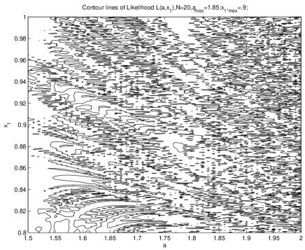
Figure 1: Contour lines of the “pure” log-Likelihood given by expression (3) for a given realization of $N=20$ data points generated with a starting value $x_{1}=0.9$, $a=1.85$ and noise std equal to $1$. The log-Likelihood landscape is similar to a 2D Brownian sheet (2D generalization of a random walk).

In addition to performing better, our “pure” ML approach does not depend on the noise level, in contrast with the ML cost function (13,14) proposed by McSharry and Smith McSharrySmith . This is an important advantage when the true level of noise is not known (noise error). Our method is insensitive to such noise error while we have found examples where the optimal estimation of the structure parameter $a$ with McSharry and Smith’s method is obtained for a value of the noise standard deviation different from the true value. In general, the true noise level is not known and McSharry and Smith’s method does not apply in such situation. Our “pure” ML method actually provides us with an estimation ${\hat{\epsilon}}$ of the standard deviation of the noise given in the last column of Table 1. These estimates have a small bias down (two fitted parameters were taken into account), which may be due to the fact that $n_{1}$ is not sufficiently large ($n_{1}=25$; $n_{2}=4$; $N=n_{1}\times n_{2}=100$).

IV Discussion of other approaches

Meyer and Christensen MeyerChristensen have proposed to replace the ad hoc construction of McSharry and Smith’s ML cost function by a Bayesian approach, assuming noninformative priors for the structural parameter $a$, for the initial value $x_{1}$ and for the standard deviation of the noise. Their approach improves significantly on McSharry and Smith McSharrySmith by recognizing the role of $x_{1}$ but turns out to be incorrect, as shown by Judd Judd , because their approach amounts to assuming a stochastic model, thus refering to quite another problem.

Based on the formulation of Berliner , Judd Judd develops a formulation which is almost identical to our “pure” ML (3) but there are important distinctions. Similarly to us, Judd introduces $x_{1}$ but he does not employ it. He prefers to eliminate the dependency on $x_{1}$ by averaging this parameter with a fiducial distribution (see e.g. KendallStuart , Chapter 21, Interval Estimation, Fiducial Intervals). Judd incorrectly calls the method based on his equations (4,5) a ML method. In fact, his equations (4,5) gives a a hybrid of ML, Bayesian and so-called fiducial methods. It is a ML method with respect to the structural parameter $a$. It is Bayesian with respect to the initial value $x_{1}$. It is fiducial since it does not assume any a-priori density for $x_{1}$, but uses a prior density function $\rho(s_{1}-w)$ (using the notation above) that is in fact a Gaussian density of the noise with mean value equal to the unknown initial value $s_{1}$. Using such density is equivalent to weighting a two-parameter likelihood by weights corresponding to different values of noise disturbances. Thus, the averaged likelihood (5) in Judd describes an ensemble of different noise disturbances of an unknown initial value $s_{1}$. This provides a (reasonable but not optimal) method of elimination of the second parameter $x_{1}$ from the maximization procedure. It is neither a pure Bayesian method (that would assume explicitly some a-priori density for $s_{1}$ which could be arbitrary, and not necessarily equal to $\rho(s_{1}-w)$), nor a ML method for two unknown parameters as we suggested above in section II.

In this context in view of the emphasis on Bayesian methods to solve this problem MeyerChristensen ; Judd , it is perhaps useful to stress that the probability theory rule $P\{A,B\}=P\{A|B\}~{}P\{B\}$ is often freely called “the Bayes rule.” This is why the averaging of likelihoods over conditional state variables can be called Bayesian approaches, although this is not quite correct since the latent (state) variables are not random values in the standard meaning of this notion (as it is assumed by McSharry and Smith), although the state variables have a limit invariant measure, as we said above. The Bayesian approach assumes that parameters are random values. For instance, McSharry and Smith assume that the latent (state) variables are random variables, which is not quite so, although the state variables have a limit invariant measure, as we said above. We stressed already that the series of state variables can be considered as a degenerate set of random values that are determined by one single random variable, namely $x_{1}$. What is more natural? To consider $x_{1}$ as a random variable with a distribution determined by the invariant measure, or to consider $x_{1}$ as an unknown parameter to be estimated? The answer, in our opinion, is dictated by consideration of efficiency: the different examples that we have explored suggest that the latter is as a rule more efficient (has smaller mean square error), at least for some combinations of sample size $N$ and noise level.

As all the above has shown, the major obstacle is the loss of information on the initial value $x_{1}$ by the unstable logistic map beyond $10-25$ time steps. We proposed the simple recipe of cutting the time series in short pieces and of averaging the estimations. Judd proposes a shadowing method Judd . It is not obvious that this will result in a consistent estimation and that this will overcome the intrinsic difficulty in treating long realizations (which is a necessary condition for unbiased estimations).

In sum, there is no analytical proof of consistency for all the estimation methods discussed until now (including the suggestions performed by the most convincing work to date Judd and our “pure” ML). It is useful to analyze the only method to our knowledge for which one can derive a proof of consistency in the present context, that is, the method of statistical moments.

V The method of statistical moments

The method of statistical moments provides a consistent estimate of the parameters for non-linear maps with ergodic properties. The method of statistical moments is the unique theoretically proven consistent estimator among all methods suggested so far by other authors. Although the moment estimates are known to have little efficiency, they are consistent! Consistency of all estimates suggested earlier including ours above were confirmed only numerically, which is very dangerous for instable non-linear maps.

We consider four moment of the observed time series: $\langle s\rangle_{N},\langle s^{2}\rangle_{N},\langle s^{3}\rangle_{N}$ and $\langle s_{i}s_{i+1}\rangle_{N}$, where the brackets stand for time averaging over some time interval $N$. Building on the knowledge that the series $\{x_{i}\}$ is ergodic Collet and using (1,2), we obtain the following relations

$$\langle s\rangle_{N} \to \langle x\rangle_{\infty}~{},$$ (6)

$$\langle s^{2}\rangle_{N} \to \langle x^{2}\rangle_{\infty}~{},$$ (7)

$$\langle s^{3}\rangle_{N} \to \langle x^{3}\rangle_{\infty}+3\langle x\rangle_{\infty}\epsilon^{2}~{},$$ (8)

$$\langle s_{i}s_{i+1}\rangle_{N} \to \langle x\rangle_{\infty}-a\langle x^{3}\rangle_{\infty}~{}.$$ (9)

Besides, averaging equation (2), we get

$$\langle x\rangle_{\infty}=1-a\langle x^{2}\rangle_{\infty}~{}.$$ (10)

This provides us with five limit relations (6-10) with five unknown parameters: $a,\langle x\rangle_{\infty},\langle x^{2}\rangle_{\infty},\langle x^{3}\rangle_{\infty}$ and $\epsilon$. Solving these five relations with respect to the unknown parameters, we get the so-called estimates of the method of moments:

$${\hat{a}} = {\langle s_{i}s_{i+1}\rangle_{N}+2\langle s\rangle_{N}-3(\langle s\rangle_{N})^{2}\over 3\langle s\rangle_{N}\langle s^{2}\rangle_{N}-\langle s^{3}\rangle_{N}}~{},$$ (11)

$$\langle{\hat{x}}\rangle_{\infty} = \langle s\rangle_{N}~{},$$ (12)

$$\langle{\hat{x}}^{2}\rangle_{\infty} = \langle s^{2}\rangle_{N}-{\hat{\epsilon}}^{2}~{},$$ (13)

$$\langle{\hat{x}}^{3}\rangle_{\infty} = {1\over{\hat{a}}}\left(\langle s\rangle_{N}-\langle s_{i}s_{i+1}\rangle_{N}\right)~{},$$ (14)

$${\hat{\epsilon}}^{2} = {\langle s^{3}\rangle_{N}-\langle x^{3}\rangle_{\infty}\over 3\langle s\rangle_{N}}~{}.$$ (15)

Because of the limit relations (6-9) (which are valid because of the ergodicity of the time series $\{x_{i}\}$ Collet ), the estimates (11-15) are consistent if $N\to\infty$.

sample size	Noise std	Estimate	$q_{1}$	$q_{2}$	$q_{2}-q_{1}$
$N$	$\epsilon$	$(a)\pm$ std
$100$	$0.05$	$1.8768\pm 0.0926$	$1.684$	$2.000$	$0.316$
$1000$	$0.05$	$1.8544\pm 0.0418$	$1.774$	$1.936$	$0.162$
$10000$	$0.05$	$1.8503\pm 0.0136$	$1.824$	$1.878$	$0.054$
$100000$	$0.05$	$1.8499\pm 0.0044$	$1.842$	$1.858$	$0.016$
$100$	$0.1$	$1.8456\pm 0.1546$	$1.499$	$2.000$	$0.501$
$1000$	$0.1$	$1.8532\pm 0.0815$	$1.693$	$2.000$	$0.307$
$10000$	$0.1$	$1.8505\pm 0.0279$	$1.795$	$1.908$	$0.113$
$100000$	$0.1$	$1.8497\pm 0.0089$	$1.833$	$1.867$	$0.034$
$100$	$0.5$	$1.2411\pm 0.7331$	$0$	$2.000$	$2.000$
$1000$	$0.5$	$1.6907\pm 0.3496$	$0.903$	$2.000$	$1.097$
$10000$	$0.5$	$1.8244\pm 0.1659$	$1.467$	$2.000$	$0.533$
$100000$	$0.5$	$1.8554\pm 0.0741$	$1.715$	$2.000$	$0.285$

Table 2: Estimation of the structural parameter $a$ by the method of statistical moments (expression (11)) for the logistic map $x_{i+1}=1-ax_{i}^{2},a=1.85$; the observations are $s_{i}=x_{i}+\eta_{i};\eta_{i}$ is a Gaussian random variable $N(0,\epsilon)$. As in table 1, $q_{1}$ and $q_{2}$ are the sample quantiles at the $2.5\%$ and $97.5\%$ probability level, so that $q_{2}-q_{1}$ gives the width of the $95\%$ confidence intervals. Each estimate for $a$ and std are based on 1000 simulated samples.

We present in table 2 the estimates of the parameter $a$ given by expression (11). The consistency of the method of statistical moments is clearly suggested by the numerical results, as seen from the bracketing of the true value by $(a)\pm$ std and by $q_{1}$ and $q_{2}$. However, as we already pointed out, the method of statistical moments is rather inefficient: the ratio of its standard deviation for $a$ to that of the “pure” ML is about $4$ for $N=100$ and $\epsilon=0.1$ for instance.

VI Concluding remarks

We have proposed a “pure” Maximum Likelihood (ML) method to estimate the structural parameter of a deterministically chaotic low-dimensional system (the logistic map), which adds the initial value $x_{1}$ to the structural parameter to be determined. We have compared quantitatively this method with the ML method proposed by McSharry and Smith McSharrySmith based on an averaging over the unknown invariant measure of the dynamical system. A key aspect of the implementation of our approach lies in the compromise between the need to use a large number of data points for the ML to become consistent and the unstable nature of dynamical trajectories which loses exponentially fast the memory of the initial condition. This second aspect prevents using our “pure” ML for systems larger than $10-25$ data points. For larger time series, we have found convenient to devide them into subsystems of very small lengths and then to average over their estimations. Numerical tests suggest that this direct ML method provides often significantly better estimates than previously proposed approaches.

The difference between McSharry and Smith’s averaging over the invariant measure and our “pure” ML is reminiscent of the distinction between “annealed” versus “quenched” averaging in the statistical physics of random systems, such as spin glasses Mezard ; dsbook . It has indeed been shown that the correct theory of strongly heterogeneous media is obtained by performing the thermal Gibbs-Boltzmann averaging over fixed structural disorder realizations, similarly to our use of a specific trajectory of the latent variables $x_{i}$’s. In constrast, performing the thermal Gibbs-Boltzmann averaging together with an averaging over different realization of the structural disorder describes another type of physics, which is not that of fixed heterogeneity. This second incorrect type of averaging is similar to the averaging of the ML over the invariant measure performed by McSharry and Smith.

There are several ways to improve our approach. One simple implementation is to use overlapping running windows. Another method is to re-estimate the realized trajectory by using the extended Kalman filter method (however, difficulties may arise due to the existence of a maximum in the logistic map). Using shadowing methods as proposed in Judd in our context would also be interesting to investigate.

Let us end with a cautionary note. As we just said, the ML approach for two parameters $(a,x_{1})$ that we suggest here evidently works only for a limited sample size N (perhaps, $N<25$ or so) due to the sensitivity upon initial conditions of the chaotic logistic map. As is well-known in classical statistics, ML-estimates have a bias that can be considerable if $N$ is not large (say, $N<100$ or so). The ML-estimates are usually only asymptotically unbiased. Thus, for $N=25$ (and all the more for $N=4$), ML-estimates can exhibit a considerable bias. Thus, averaging biased estimates as we proposed many not result in a consistent estimation. Therefore, we cannot assert that our ML method (as well as any other suggested methods) is consistent. We can only observe, for particular combinations of the considered parameters, the numerically determined mean square error of our suggested estimates with respect to the true parameter value. We are pleased if these errors are not too high, although our estimates can be biased (though, with small bias). But we are not able to make such bias arbitrarily small by increasing the sample size $N$, due to the instability under the iterations of the logistic map which leads to a loss of information about the initial value $x_{1}$. Thus, the situation is rather hopeless for the establishment of a meaningful statistical theory of estimation using the continuous theory of classical statistics to such discontinuous objects as the invariant measures of chaotic dynamical systems.

Appendix A: One-step and total least-square estimations

McSharry and Smith noticed that the one-step leasts-square method gives strongly biased results for the estimation of $a$ McSharrySmith . Indeed, the method of estimation of the parameter $a$ by the one-step least square method is evidently inconsistent, since the deviations (of the random variables) to be minimized in a least-square sense are

$$s_{i+1}-F(s_{i},a) = x_{i+1}+\eta_{i+1}-F(x_{i}+\eta_{i},a)$$ (16)

$$= \eta_{i+1}+2ax_{i}\eta_{i}+a\eta_{i}^{2}~{},$$

which has non-zero expectation equal to $a\epsilon^{2}$. But, the fundamental least-square principle consists in the minimization of deviations with zero mean. There are no least-square schemes that would suggest to minimize random deviations with non-zero mean depending on an unknown parameter. Thus, it is not reasonable to include the least-square method in any reasonable comparison.

The method called by McSharry and Smith as “total least-squares” (TLS) is applied in situation when the variables $x_{i}$ are known only with some errors $\eta_{i}$. This situation is called in statistics a “Confluence analysis,” or “Estimation of a structural relation between two (or more) variables in the presence of errors on both variables” FrischR ; Geary ; KendallStuart . In such a situation of confluence analysis, since the $x_{i}$’s are in fact unknown (nuisance) parameters whose number grows with sample size, there is no guarantee of consistency of the ML estimates of the structural parameter $a$.

As an example, let us consider the very simple confluent scheme:

$$Y_{i} = X_{i}+\eta_{i}~{},$$ (17)

$$Z_{i} = X_{i}+\zeta_{i}~{}.$$ (18)

Suppose we observe a sample of $N$ pairs $(Y_{i},Z_{i}),i=1,...,N$, where $X_{i}$ are unknown arbitrary values and $\eta_{i},\zeta_{i}$ are iid Gaussian random variables with standard deviation $\epsilon$. The problem consists in estimating the parameter $\epsilon$. Similarly to the situation with (1) and (2) studied in McSharrySmith , no restrictions are placed on the $X_{i}$’s. The likelihood $L(\epsilon,X_{1},...,X_{N}|(Y_{i},Z_{i}),i=1,...,N)$ is

$$L(\epsilon,X_{1},...,X_{N}|(Y_{i},Z_{i}),i=1,...,N)\propto$$

$$\epsilon^{-2N}~{}\exp\left[-(1/2\epsilon^{2})\sum_{i=1}^{N}(Y_{i}-X_{i})^{2}-(1/2\epsilon^{2})\sum_{i=1}^{N}(Z_{i}-X_{i})^{2}\right]~{}.$$ (19)

The MLE ${\hat{X}}_{i}$’s of the $X_{i}$’s (that coincide in this case with the least-square estimates) are:

$${\hat{X}}_{i}={Y_{i}+Z_{i}\over 2}~{}.$$ (20)

Inserting (20) into (19), we get

$${\hat{L}}(\epsilon|(Y_{i},Z_{i}), i=1,...,N)\propto$$ (21)

$$\epsilon^{-2N}~{}\exp\left[-(1/4\epsilon^{2})\sum_{i=1}^{N}(Y_{i}-Z_{i})^{2}\right]~{}.$$

Thus, the MLE of the parameter $\epsilon$ obtained from (21) satisfies

$$\epsilon^{2}={1\over 4N}\sum_{i=1}^{N}(Y_{i}-Z_{i})^{2}~{}.$$ (22)

Since ${\rm E}\left[(Y_{i}-Z_{i})^{2}\right]=2\epsilon^{2}$, the estimate (22) is inconsistent. A consistent (“corrected”) estimate is

$$\epsilon^{2}={1\over 2N}\sum_{i=1}^{N}(Y_{i}-Z_{i})^{2}~{}.$$ (23)

Thus, we see that the MLE of the structural parameter $\epsilon$ is inconsistent due to the increasing number of nuisance parameters. Thus, the direct use of the least-square (or total least-square) in the confluent situation is not justified, and was not recommended in any statistical textbook. Instead, standard statistical works recommend a “corrected” ML estimates (see for instance Geary ; KendallStuart ).

We should stress in addition that there is a significant difference between the standard confluent analysis and the problem addressed in McSharrySmith . Confluent analysis deals with arbitrary unknown (distorted) arguments $x_{i}$, whereas in McSharrySmith , the latent variables $x_{i}$ are related by the non-linear map (2). The information on the structure of the $x_{i}$’s is not used in Confluence Analysis while it can really help in the estimation procedure as shown in McSharrySmith and in the present work.

References

- (1) P.E. Mcsharry and L.A. Smith, Phys. Rev. Lett. 83, 4285 (1999)
- (2) Frisch R. Statistical Confluence Analysis by Means of Complete Regression Systems, Oslo, 1934.
- (3) Geary R.C. Non-linear functional relationship between two variables when one variable is controlled, J. Amer. Statist. Ass. 48, 94 (1953).
- (4) M. Kendall and A. Stuart, The advanced theory of statistics, Curvilinear Dependencies, 2d ed. (New York, Hafner Publ. Co., 1961), Chapter 29, Section 29.50.
- (5) D. Sornette and A. Arnéodo, J. Phys. (Paris) 45, 1843 (1984).
- (6) S.C. Phatak and S.S. Rao, Phys. Rev. A. 51 (4 Part B), 3670 (1995).
- (7) R. Meyer and N. Christensen, Phys. Rev. E 62, 3535 (2000).
- (8) CK. Judd, Phys. Rev. E 67 (2), 026212 (2003).
- (9) M.L. Berliner, J. Am. Stat. Assoc. 86, 939 (1991).
- (10) P. Collet and J.-P. Eckmann, Iterated maps on the interval as dynamical systems (Basel; Boston: Birkhauser, 1980).
- (11) M., Mézard, M., Parisi, G. and Virasoro, M., Spin Glass Theory and Beyond (World Scientific, Singapore, 1987).
- (12) D. Sornette, Critical Phenomena in Natural Sciences (Springer Series in Synergetics, Heidelberg, 2000), see chapter 16.