Data compression using correlations and stochastic processes in the ALICE Time Projection chamber

Abstract

In this paper lossless and a quasi lossless algorithms for the online compression of the data generated by the Time Projection Chamber (TPC) detector of the ALICE experiment at CERN are described.

The first algorithm is based on a lossless source code modelling technique, i.e. the original TPC signal information can be reconstructed without errors at the decompression stage. The source model exploits the temporal correlation that is present in the TPC data to reduce the entropy of the source.

The second algorithm is based on a lossy source code modelling technique, i.e. it is lossy if samples of the TPC signal are considered one by one. Nevertheless, the source model is quasi-lossless from the point of view of some physical quantities that are of main interest for the experiment. These quantities are the shape, the location of the center of gravity as well as the total charge of the signal.

In order to evaluate the consequences of the error introduced by the lossy compression, the results of the trajectory tracking algorithms that process data offline are analyzed, in particular, with respect to the noise introduced by the compression. The offline analysis has two steps: cluster finder and track finder. The results on how these algorithms are affected by the lossy compression are reported.

In both compression technique entropy coding is applied to the set of events defined by the source model to reduce the bit rate to the corresponding source entropy. Using TPC simulated data, the lossless and the lossy compression achieve a data reduction to 49.2% of the original data rate and respectively in the range of 35% down to 30% depending on the desired precision.

In this study we have focused on methods which are easy to implement in the frontend TPC electronics.

I Introduction

ALICE (A Large Ion Collider Experiment) is an experiment that will start in 2007 at the LHC (Large Hadron Collider) at CERN TPCTDR ; alicewww . The experiment will study collisions between heavy ions with energies around 5.5 TeV per nucleon. The collisions will take place at the center of a set of several detectors, which are designed to track and identify the produced particles.

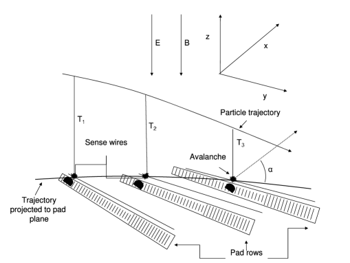
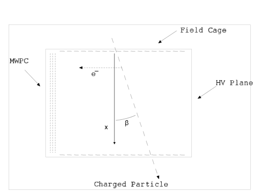
Figure 1: Schematic view of the detection process in TPC (upper part - perspective view, lower part - side view).

One of the main detectors of the ALICE experiment is the Time Projection Chamber (TPC). Its task is track finding, momentum measurement and particle identification by d$E$/d$x$. Good two-track resolution, required for correlation studies, is one of the main design goals.

The TPC is a large horizontal cylinder, filled with gas, where a suitable axial electric field is present. When particles pass through, they ionize the gas atoms, and the resulting electrons drift in the electric field. By measuring the arrival of electrons at the end of the chamber, the TPC can reconstruct the path of the original charged particles. The electrons are collected by more than 570 000 sensitive pads where they create signals. These signals are amplified by a preamplifier–shaper and digitalized by a 10-bit A/D converter at a sampling frequency of 5.66 MHz. The digitalized signal is processed and formatted by an Application Specific Integrated Circuit (ASIC) called ALTRO (ALICE TPC Read-Out) musa00altro . At this stage, the overall throughput of the 570 000 channels is around 8.4 GByte/s.

The total amount of the TPC data is expected to be about 1 PBy per year. In order to keep the complexity and cost of the data storage equipment as low as possible, we have to reduce the volume of data using suitable data compression methods. The cost reduction of the data storage system is roughly proportional to the data compression factor. Furthermore, it is better to implement the compression system in the front-end electronics at the output of the ALTRO circuit, so that the cost for the optical links, which carry data out of the chamber to the following stages of the acquisition chain, could be also reduced.More sophisticated methods for TPC data compression based on online tracking, which will be used further in data acquisition chain are developed in Bergen and Heidelberg bergen .

The use of a lossy source model, justified by the fact that generally it can provide significantly higher compression ratios compared to lossless models, has the drawback that some deterioration in the reconstruction of data must be accepted. Lossy source models have become very popular in the last decade in the field of audio and video compression for their remarkable performance. Lossy models have been carefully designed so that reconstruction distortions are not perceived using psychovisual or psychoacoustic models or they remain comparable with the intrinsic signal noise.

Obviously, for physical data, psychovisual or psychoacoustic tests are meaningless or even not applicable since the TPC signal is not to be observed by the human eye or ear. In nicolaucig02 , the compression noise introduced on the sample values by the described lossy or quasi lossless techniques has been evaluated in terms of RMS of the introduced Error (RMSE).

However, in this case, the RMSE, despite being a simple and well known distortion measure, is not very useful. The fundamental information that has to be extracted from TPC data are not sample values themselves but the physical quantities that enable the reconstruction of particle trajectories. Therefore, the correct way to evaluate the importance of the distortion introduced by the compression–decompression process has to be related to the high level information that is carried by the data. In particular, TPC data are collected with the objective of measuring particle energy and trajectory.

Therefore, the most effective way to estimate the consequences of the compression distortion error, is to observe how the extraction of energy and trajectories are affected by the compression–decompression process. A simple way to obtain these estimates is to apply the cluster finding and tracking algorithms on both simulated data and their compressed–decompressed version and compare the results.

This article is arranged in the following way. In section II, all stochastic processes relevant for particle detection in ALICE TPC are briefly described. In section III, TPC data format is specified. In section IV, different lossless compression techniques are described and their efficiencies are compared. In section V, the fast one dimensional lossy compression technique is shown and the impact of compression–decompression to the distortion of most important physical quantities is demonstrated.

II Stochastic processes in TPC

II.1 Ionization in gas

A charged particle that traverses the gas of the chamber leaves a track of ionization along its trajectory. The collisions with the gas atoms are purely random. They are characterized by a mean free path $\lambda$ between ionizing encounters, which is given by the ionization cross-section per electron $\sigma_{\rm{ion}}$ and the density N of electrons:

$$\lambda=1/(N\sigma_{\rm{ion}}).$$

Therefore, the number of encounters along the length L has the mean of $L/\lambda$, and the frequency distribution is given by Poisson distribution

$$P(L/\lambda,k)=\frac{(L/\lambda)^{k}}{k!}\exp(-L/\lambda).$$

The mean free path $\lambda$ is given by the properties of the gas and by charged particle characteristics:

$$\lambda=\frac{1}{N_{\rm{prim}}{\times}f(\beta\gamma)},$$

where $N_{\rm{prim}}$ is the number of primary electrons per cm produced by a Minimum Ionizing Particle (MIP), and $f(\beta\gamma)$ is Bethe–Bloch curve.

II.2 Generation of secondary electrons

The energy loss $E_{\rm{tot}}$ released in primary ionization to atomic electrons is a random variable. It can be described by Photo-Absorbtion Ionization model (PAI). In most cases, if one neglects the atomic shell structure, at sufficiently high $E_{\rm{tot}}$ (the energy where the atomic shell structure is not more important) it obeys $1/E_{\rm{tot}}^{2}$ rule.

If the electron produced by the charged particle has sufficient kinetic energy $E_{\rm{tot}}$, it will produce secondary electrons creating thus electron cluster. The mean total number of electrons in such cluster is given by:

$$N_{\rm{tot}}=\frac{E_{\rm{tot}}-I_{\rm{pot}}}{W_{\rm{ion}}}+1,$$

where $E_{\rm{tot}}$ is the energy loss in a primary collision, $W_{\rm{ion}}$ is the effective energy required to produce an electron–ion pair and $I_{\rm{pot}}$ is the first ionization potential. The random character of the secondary ionization process smears out structures in $E_{\rm{tot}}$ spectra, atomic shell structure behavior is suppressed. For example in the gas mixture 90% Ne, 10 % CO₂ the $E^{-2.2}_{\rm{tot}}$ effective parametrization at lower $E_{\rm{tot}}$ can be used.

II.3 Diffusion of electrons

Produced electrons drift through the gas with an effective constant drift velocity in the direction given by the electric field $\mathbf{E}$ and magnetic field $\mathbf{B}$ (which we assume are parallel to z-direction). Drifting electrons are scattered on the gas molecules so that their direction of motion is randomized in each collision. The position of the electron, after drifting over a distance $L_{\rm{drift}}$, can be described by 3-D Gaussian distribution:

$$P(x,y,z)=\frac{1}{\sqrt{2\pi}\sigma_{\rm{T}}}\exp\left[-\frac{(x-x_{0})^{2}}{2\sigma_{\rm{T}}^{2}}\right]$$

$$\frac{1}{\sqrt{2\pi}\sigma_{\rm{T}}}\exp\left[-\frac{(y-y_{0})^{2}}{2\sigma_{\rm{T}}^{2}}\right]$$

$$\frac{1}{\sqrt{2\pi}\sigma_{\rm{L}}}\exp\left[-\frac{(z-L_{\rm{drift}})^{2}}{2\sigma_{\rm{L}}^{2}}\right],$$ (1)

where $\{x_{0},y_{0},z_{0}\}$ is the electron creation point and transversal diffusion $\sigma_{\rm{T}}$ respectively longitudinal diffusion $\sigma_{\rm{L}}$ are given by drift length $L_{\rm{drift}}$ and gas coefficient $D_{\rm{T}}$ and $D_{\rm{L}}$

$$\sigma_{\rm{T}}=D_{\rm{T}}\sqrt{L_{\rm{drift}}},$$

$$\sigma_{\rm{L}}=D_{\rm{L}}\sqrt{L_{\rm{drift}}}.$$

II.4 $\mathbf{E{\times}B}$ and unisochronity effect near the anode wires

It has been assumed that the electric and magnetic fields in the drift volume are uniform and parallel. This, however, is not true close to the anode wires, where the electric field becomes radial. Thus the electrons experience a shift along the wire direction (due to the Lorentz force). If an electron enters the readout chamber at the point $(x_{\rm{e}},y_{\rm{e}})$, it is displaced in the x-direction (assuming that the wires are placed along y-axis). The new y-position of the electron is then given by

$$y=y_{\rm{e}}+\omega\tau\cdot(x-x_{\rm{e}})\>,$$

where $x$ is the coordinate of the wire on which an electron is collected, and $\omega\tau$ is the tangent of Lorentz angle ($\mathbf{E{\times}B}$ effect). The drift length which determines z coordinate will be also affected, because of change in the path to the anode wire (unisochronity effect).

II.5 Signal generation

Inside the readout chamber, as an electron drifts towards the anode wire, it travels in an increasing electric field. Once the electric field is strong enough that between collisions with the gas molecules the electron can pick up sufficient energy for ionization, another electron is created and the avalanche starts. As the number of electrons multiplies in successive generations, the avalanche continues to grow until all the electrons are collected on the wire. The resulting number of electrons created in the avalanche, can be described by an exponential probability distribution

$$P(q)=\frac{1}{\overline{q}}\cdot\exp{-\frac{q}{\overline{q}}}\>,$$

where $\overline{q}$ is the average avalanche amplitude.

An electron avalanche collected on the anode wire induces a charge on the pad plane. This charge is integrated over the pad area. The time signal is obtained by folding the pad response to the avalanche with the shaping function of the preampamplifier–shaper. This signal is then sampled with a constant frequency. On the top of sampled signal a random electronic noise is superimposed.

As a result a charged particle interacting with gas generates a cluster of amplitudes. This cluster is used for later estimation of local track position and of local energy deposition. The shape of the cluster is used as additional information for the estimation of position uncertainties and for the estimation of the overlap factor between two tracks.

II.6 Accuracy of local coordinate measurement

The accuracy of the coordinate measurement is limited by a track angle which spreads ionization and by diffusion which amplifies this spread.

The track direction with respect to pad plane is given by two angles $\alpha$ and $\beta$ (see fig. 1). For the measurement along the pad-row, the angle $\alpha$ between the track projected onto the pad plane and pad-row is relevant. For the measurement of the the drift coordinate (z–direction) it is the angle $\beta$ between the track and z axis.

The ionization electrons are randomly distributed along the particle trajectory. Fixing the reference x position of a electron at the middle of pad-row, the y (resp. z) position of the electron is random variable characterized by uniform distribution with the width $L_{\rm{a}}$, where $L_{\rm{a}}$ is given by the pad length $L_{\rm{pad}}$ and the angle $\alpha$ (resp. $\beta$):

$$L_{\rm{a}}=L_{\rm{pad}}\tan\alpha$$

The diffusion smears out the position of the electron with gaussian probability distribution with $\sigma_{\rm{D}}$. Contribution of the $\mathbf{E{\times}B}$ and unisochronity effect is in the case of Alice TPC negligible.

The accuracy of the position measurement can be expressed as:

$\sigma_{\rm{z}}$ of cluster center in z (time) direction:

$$\sigma^{2}_{\rm{z_{COG}}}=\frac{D^{2}_{\rm{L}}L_{\rm{drift}}}{N_{\rm{ch}}}G_{\rm{g}}+{}$$ (2)

$${}\frac{\tan^{2}\alpha~{}L_{\rm{pad}}^{2}G_{\rm{Lfactor}}(N_{\rm{prim}})}{12N_{\rm{chprim}}}+\sigma^{2}_{\rm{noise}}$$

and $\sigma_{\rm{y}}$ of cluster center in y(pad) direction:

$$\sigma^{2}_{\rm{y_{COG}}}=\frac{D^{2}_{\rm{T}}L_{\rm{drift}}}{N_{\rm{ch}}}G_{\rm{g}}+{}$$ (3)

$${}\frac{\tan^{2}\beta~{}L_{\rm{pad}}^{2}G_{\rm{Lfactor}}(N_{\rm{prim}})}{12N_{\rm{chprim}}}+\sigma^{2}_{\rm{noise}}$$

where ${N_{\rm{ch}}}$ is the total number of electrons in cluster, ${N_{\rm{chprim}}}$ is the number of primary electrons in cluster, ${G_{\rm{g}}}$ is the gas gain fluctuation factor parametrization, ${G_{\rm{Lfactor}}}$ is the secondary ionization fluctuation factor and $\sigma_{\rm{noise}}$ describe the contribution of the electronic noise and ADC quantization to the resulting sigma of the COG.

The typical resolution in the case of ALICE TPC is on the level of $\sigma_{\rm{y}}\sim$ 0.8mm and $\sigma_{\rm{z}}\sim$ 1.0mm integrating over all clusters in the TPC.

II.7 Accuracy of the total amplitude measurement

The total charge deposited in the clusters can be used for particle identification. The important value, which is specific for different particle types and different particle momenta, is the number of primary collision per unit length, $N_{\rm{chprim}}$. $N_{\rm{chprim}}$ is a random variable described by Poisson distribution. Due to the secondary ionization and gas gain fluctuations the total charge is described by very broad Landau distribution.

III The ALICE TPC read-out data format

Before describing the compression algorithm, it is necessary to spend a few words on the format of data at the output of ALTRO circuit, in order to understand how the compression algorithms are applied. Such data are indeed the input of the compression system TPCTDR ; musa00altro .

In the ALTRO data format only the samples over a given threshold are considered, while the others are discarded. This means that, if we call bunch a group of adjacent over-threshold samples coming from one pad, the signal can be represented “bunch by bunch”. More precisely, a bunch is described by three fields: temporal information (temporal position of the last sample in the bunch), one 10-bit word, bunch length (i.e. the number of samples in the bunch, one 10-bit word), and sample amplitude values (few 10-bit words).

IV Lossless compression of TPC signals

The lossless techniques of the data compression are based on the fact that TPC sample values (ADC and temporal) are not equally probable. A theoretical lower limit on the average word size using Huffman codding, or arithmetic coding lossless technique is given by entropy of the data source:

$$\ E(p)=\sum{p(A)\log_{\rm{2}}p(A)}$$ (4)

The lossless techniques described in this paper are based mainly on an appropriate probability model for each data field of the ALTRO data format. Specific probability models for each sample in a bunch were developed. These models intend to capture both temporal correlation among samples and the characteristic shape of TPC electrical pulses.

IV.1 Time information

As already mentioned, in the ALTRO data format time information is represented as the 10-bit number of the time-bin of the last sample of the bunch. The probability distribution of this variable is roughly uniform. In order to achieve better compression ratio this variable is substituted by the distance between two consecutive bunches. The probability of this variable is described by exponential distribution with much lower entropy factor. The entropy of temporal information is given by mean distance between two bunches. It depends on the event multiplicity, noise level and local occupancy, which is known function of the pad-row radius. In order to optimize entropy coding, it will be necessary to investigate probability distribution as a function of track multiplicity. This information will be known from other faster ALICE detectors.

The mean number of bits used for the coding of time information is roughly 4.9 bits for the full event with maximal track density. Using different codes in different places inside TPC, an additional 6% reduction in time information can be achieved.

IV.2 Bunch length

In the ALTRO data format, the bunch length is represented as a 10-bit code number of samples in the bunch. The bunch length depends on the diffusion, the angular effect and the total deposited energy. There is no apparent correlation with data coded before. Small diffusion for short drift length is compensated by big angular effect. The total deposited energy is known only after coding of the bunch length. Since no apparent correlation with other data (e.g. length of adjacent bunches) exists and no better model (i.e. a model of events with lower entropy) could be found, this information is coded directly.

IV.3 Sample values coding

Sample values are the main contribution to the resulting data volume. This subsection describes, first a basic model, and then introduces a more sophisticated one, that can provide higher performances in terms of compression efficiency.

Data compression can be obtained by directly applying entropy coding to the sample values without any modelling of the information source. This method will be referred bellow (in table 2) as Entropy Coding (EC).

IV.4 Coding model based on the sample position

Improvements in compression performance can be obtained by appropriate modelling. A first improvement has been achieved by the fact that the statistics of the signal sample values depend on the position of the sample itself in the bunch.

Bunch length	freq	0	1	2	3	4
1	136	2.21
2	279	4.04	4.04
3	422	4.64	5.5	4.64
4	241	4.18	6.67	6.02	4.18
5	53	3.83	6.1	7.15	6.1	3.83

Table 1: Entropy of the sample data as a function of the sample position in the bunch. Frequency of the sample length is given in arbitrary units.

Due to the pseudo Gaussian shape of most of the bunches, the first and the last sample of each bunch are likely to have a smaller value with respect to those in central positions. Similarly, small values are also expected for isolated samples, i.e. belonging to one-sample bunches (see table 1).

Therefore, a classification of the samples into three classes was chosen: one class for isolated samples, one for samples at the beginning and at the end of multiple sample bunches, and the last for samples in the central positions of a bunch. Using three different probability distributions for entropy coding the sample values can be coded more efficiently than using only one probability distribution. This coding scheme will be referred in table 2 as coding using Sample Position (SP).

IV.5 Source models exploiting temporal correlation

Improvement on compression performances can be expected by exploiting temporal correlation, i.e. the correlation between consecutive samples; this can be done by implementing a suitable prediction scheme.

This approach is explained on the example, where a three-sample bunch is considered. Let us assume that the first two samples have already been coded and that the third one has to be coded. The code to be used for sample No. 3 may be chosen among eight possible codes according to the value of sample No. 2. In particular, this is done by subdividing the range of sample No. 2 (i.e. 0. . . 1023) into different intervals, and associating a different code (for the third sample) to each of these intervals.

This conditioned probability model can be extended to all the samples that are not in the first position in the bunch and for any bunch length. However, if the real-time implementation constraints are taken into account, and, in particular, the need to reduce the memory size of the model, it is not good to have an exceedingly large number of codes. Consequently, samples are partitioned into four classes only, to keep the complexity of the model low. This limitation does reduce the efficiency of the model but the reduction is only of the order of 0.6%. This coding scheme will be referred in table 2 as coding using Temporal Correlation (TC).

IV.6 Comparison of different lossless technique

	Time	Length	Samples	Total
Altro	10 bits	10 bits	38.1 bits	58.1 bits(100%)
EC	4.9 bits	3.1 bits	22.4 bits	30.3 bits (52.5%)
SP	4.9 bits	3.1 bits	21.3 bits	29.2 bits (50.3%)
TC	4.9 bits	3.1 bits	20.7 bits	28.6 bits (49.2%)

Table 2: Performance of several lossless techniques compared to the zero suppressed ALTRO data format. ALTRO: original ALTRO data; EC: entropy coding of sample values, bunch length, and time information; SP: classification of samples according to their position (3 code tables used); TC: coding technique that exploits temporal correlation (20 code tables used). Numbers in the columns represent the number of bits per bunch dedicated to each field; numbers in the right column represent the overall number of bits per bunch, and, in parenthesis, the size with respect to the original ALTRO data format.

The results of different lossless approaches on simulated TPC data are shown in table 2. It may be noticed that the latter TC technique provides a compression of data down to 49.2% of the original size. Even this best technique provides reduction factor only by 3% better then direct EC technique.

Additional attempt tried to use predicted mean cluster shape information. Knowing the position of the bunch, the diffusion given by drift length ($L_{\rm{drift}}$) and inclination angle for primary particles are known. However, due to the fluctuation of cluster shape and due to the large amount of secondary particles with unknown angles, this prediction is not very good, and the entropy of the samples is reduced only by additional factor 2%.

IV.7 Space correlation

In the trial to exploit space correlation, three lossless models have been considered. The first is based on spatially conditioned probability, the second on a predictive model, third on 2-dimensional cluster finder, with residual saving.

The first one is the equivalent, in the spatial domain, to what has been done for time correlation. Different codes are available to code the samples; for each sample, the appropriate code is selected according to the value of the samples in the same time-bin but in adjacent pads. This method provides poorer performance when compared with the one which exploits time correlation (the comparison being done using the same model complexity, i.e. number of probability distributions available in memory). Moreover, these two techniques cannot be easily combined, i.e. it is difficult to exploit both temporal and spatial correlations at the same time, because this would require a very large number of probability distributions (i.e. code tables).

The second method that has been investigated uses the prediction of the sample values from the samples in adjacent pads and coding the error of this prediction. Unfortunately, also for this model, the performance is not very good.

Pulses in one pad-row often resemble temporally shifted versions of those in the adjacent pad-row. The two methods described above have been modified by adding the first stage which shifts pulses so as to increase spatial correlation with adjacent. Although the performance has slightly improved, the increase of the compression efficiency was lower than expected. The correlations are relatively small. The main problems here are in the big amount of secondary particles crossing TPC with unknown $\beta$ angle (not pointing to the primary vertex), big spread of the particle momenta (unknown $\alpha$ angle) and the Landau fluctuation of deposited energy on different pad rows, which is almost uncorrelated. Moreover, the position of the original track relative to the pad, affects the correlation by a large factor. The signal amplitude in adjacent pads and adjacent pad-rows are very weakly correlated, unless the position and direction of the track is known.

In order to get better knowledge of the track position, two-dimensional cluster finding can be done before. The entropy of the stored residuals is by 30% lower than entropy of the original samples but there are problems with the track overlaps and with description of the cluster topology (i.e. where to store residuals).

Based on these results we conclude that it is not simple to exploit spatial correlation (i.e. correlations between adjacent channels). There might be more sophisticated and complex lossless models able to exploit it, but relatively simple models seem to fail.

V Lossy compression of TPC signals

V.1 Fluctuation and accuracy of the amplitude measurement

The number of primary ionization electrons produced by the charged particle in the gas is the random variable described by Poisson distribution with the mean value  14.35 $\rm{cm^{-1}}$ for minimum ionizing particle in the gas of Alice TPC. The secondary electron production (described by  $E^{-2.2}$ probability distribution) increases the number of produced electrons. Maximum probable value is 25 $\rm{cm^{-1}}$ of total electrons. This effect also smears probability distribution to the relatively broader Landau distribution.

Due to the angular effect and diffusion, electrons are distributed among several time-bins and pads. The number of electrons which contributes to the given pad and time-bin is described roughly by Poisson distribution. Each of the registered electrons is subject of gas multiplication which is described by exponential probability distribution. Over this, additional electronic noise is superimposed to each signal.

If we fix the track position and the number of primary electrons, the remaining sample uncertainties can be in the first approximation estimated as:

$$\ \sigma_{\rm{S}}=\sqrt{\sigma_{\rm{noise}}^{2}+G{\times}A}$$ (5)

where $\sigma_{\rm{noise}}$ is given by electronic noise and sampling imprecision, and G is the gain conversion factor.

The situation is more complicated, data samples are correlated through the time response function and the pad response function. The relative correlation between the samples depends on the ratio of the width of the response functions to the width given by stochastic processes.

	no	$K_{\rm{off}}$=1	$K_{\rm{off}}$=1.5	$K_{\rm{off}}$=1
		$K_{\rm{cor}}$=1	$K_{\rm{cor}}$=1.5	$K_{\rm{cor}}$=2
range	0..1024	0..62	0..42	0..33
entropy	5.7	3.89(3.39)	3.34(2.84)	2.92(2.45)
$\sigma_{\rm{P}}$	1.000	1.000	1.006	1.030
$\sigma_{\rm{T}}$	1.000	1.005	1.015	1.04
$\sigma_{\rm{PRF}}$	0.069	0.070	0.071	0.074
$\sigma_{\rm{TRF}}$	0.079	0.079	0.081	0.083
Gain	4.61$\pm$0.69	4.63$\pm$0.70	4.64$\pm$0.71	4.66$\pm$0.72

Table 3: The influence of the lossy compression with different lossy parameters to the cluster characteristic. In row 1 effective range mapping shown. Entropy of the samples are shown in row 2. Numbers in parenthesis represent effective entropy od data sample, using different code table for different sample position in the bunch. In row number 3 and 4 ($\sigma_{\rm{P}}$ and $\sigma_{\rm{T}}$) the influence of the lossy compression to the cluster space resolution in pad respectively in time direction is shown. Row number 5 and 6 shows the relative influence of compression to the shape of cluster in time and pad directions. Gain row show the reconstructed ratio between total deposited energy and numbers of contributing electrons to the cluster.

	no	$K_{\rm{off}}$=1	$K_{\rm{off}}$=1.5	$K_{\rm{off}}$=1
		$K_{\rm{cor}}$=1	$K_{cor}$=1.5	$K_{\rm{cor}}$=2
$\sigma_{\phi}$[mrad]	1.399$\pm$0.030	1.378$\pm$0.030	1.406$\pm$0.030	1.403$\pm$0.03
$\sigma_{\Theta}$[mrad]	0.997$\pm$0.018	0.992$\pm$0.018	1.002$\pm$0.018	0.989$\pm$0.018
$\sigma_{p_{\rm{t}}}$[%]	0.881$\pm$0.011	0.885$\pm$0.011	0.886$\pm$0.011	0.905$\pm$0.011
$\sigma_{{\rm{d}}E/{\rm{d}}x}$[r.u]	2.96$\pm$0.11	2.98$\pm$0.11	3.06$\pm$0.11	3.20$\pm$0.11

Table 4: The influence of the lossy compression with different lossy parameters on the track characteristics.

V.2 Dynamic precision of the digitization

In the following study, dynamic precision of sample quantization was investigated. The quantization was chosen to correspond to the sample deviation, modifying formula (5) to:

$$\ \delta_{\rm{d}}=\sqrt{K_{\rm{off}}^{2}+K_{\rm{cor}}^{2}{\times}A}$$ (6)

where $K_{\rm{off}}$ and $K_{\rm{cor}}$ factors were chosen as free parameters. $K_{\rm{off}}$ is proportional to the electronic noise and $K_{\rm{cor}}$ is given by statistics of the stochastic processes and by correlations. Different combinations of these factors were investigated.

In table 3 the influence of different quantization on the precision of the cluster characteristic determination is shown.

The gain factor $G=A_{\rm{t}}/N_{\rm{el}}$ ($A_{\rm{t}}$ is the total charge in cluster, $N_{\rm{el}}$ is the number of electrons contributing to the cluster) measures the precision of the local deposited energy determination. This factor is important for d$E$d$x$ measurement and consequently for particle identification (PID). The influence of the compression on the cluster position determination varies between 0 to 4%, depending on the compression factor, as can be expected. The shape of the cluster ($\sigma_{\rm{PRF}}$ and $\sigma_{\rm{TRF}}$), important for cluster quality determination, varies between 1 to 6%.

In table 4 the influence of the compression on the tracking is shown. Reported distortions in $p_{\rm{t}}$ and angular resolution are slightly smaller than in the case of the cluster position(0% up to 3.5%) . This is due to the other stochastic processes which contribute to the track parameters e.g. the multiple scattering. For high-momentum particles, where the influence of multiple scattering is not so important, the expected distortion will be determined by the cluster position distortions.

Reducing the number of the possible sample values, vector quantization of bunches were also investigated. Additional reduction factor of $\sim$6% was achieved on top of the results reported in table 3.

VI Conlusions

Several methods of lossless TPC data compression was investigated (sec. IV.6). The best one dimensional methods provide compression factor down to 49.2%.

A lossy compression approach for the data generated by the TPC chamber in the ALICE experiment has been also investigated. The main idea was to preserve, on the level intrinsic noise, the three more important local quantities: the cluster position, the deposited energy and the shape of the cluster. Keeping the distortions of the local quantities at a reasonable level, the impact on the most interesting physical quantities, particle momenta and d$E$d$x$ is minimal. This approach achieves compression rates in the range from 35% down to 30%, depending on the desired precision. In this study we have focused on methods which are easy to implement in the frontend TPC electronics.

References

- (1) ALICE Collaboration, ALICE Technical Design Report of the Time Projection Chamber
- (2) ALICE – A Large Ion Collider Experiment,http://na49info.cern.ch/alice/html/detector
- (3) L. Musa and R. E. Bosch, Alice TPC Readout chip, Internal Note,2000
- (4) TPC data compression, NIM A 489(2002),406-421
- (5) A. Nicolaucig,Compressione dei dati generati dalla Time Projection Chamber nell’esperimento ALICE presso il CERN,2000