General properties and analytical approximations of photorefractive solitons

Abstract

We investigate general properties of spatial $1$-dimensional bright photorefractive solitons and suggest various analytical approximations for the soliton profile and the half width, both depending on an intensity parameter $r$.

I Introduction

One-dimensional bright photorefractive solitons have been the subject of numerous investigations by experimental and theoretical physicists Segev et al. (1992, 1994); Duree et al. (1993). While experimentalists are primarily concerned with half width measurements leading to so-called “existence curves” Segev et al. (1996), there is also a theoretical interest in additional properties of these solitary waves, such as the form and the asymptotic behavior of the soliton profile with respect to large distances or extreme values of its parameters. In view of the lack of exact solutions of the relevant partial differential equation there is hence a strong desire for proper approximations that suit the needs of both groups of physicists alike.

To our knowledge, there is only one published approach to analytically approximating the soliton profile, namely Montemezzani and Günter (1997). But this approach is not the only possible one: In the present paper we will provide alternative approximations and discuss their respective virtues. Further we will prove some general basic properties of photorefractive solitons which are independent of the chosen approximation.

The starting point for our investigations is the theory developed by Christodoulides and Carvalho Christodoulides and Carvalho (1995) in which the profile $f(x)$ of bright spatial photorefractive solitons is described by the following dimensionless differential equation (cf. eq.(19) in Christodoulides and Carvalho (1995)):

$$f_{xx}+\beta F(f)=0,$$ (1)

where

$$F(f)=2f\left(\frac{\ln(1+r)}{r}-\frac{1}{1+rf^{2}}\right).$$ (2)

Here $f$ is proportional to the electric field normalized to the maximal value $1$, $r$ represents the ratio of intensity to dark intensity of the beam and $x$ is the coordinate transversal to the direction of the light beam. Since the factor $\beta$ can be compensated by an appropriate scaling of the $x$-axis, i. e. $x\to\sqrt{\beta}x$, we will choose $\beta=1$ throughout the rest of the paper. Thus $r>0$ is the only parameter the soliton profile $f(x)$ is depending on.

For the derivation of this nonlinear wave equation and the pertinent simplifications we refer the reader to the original paper Christodoulides and Carvalho (1995).

Appropriate initial conditions for (1) are

$$f(0)=1,\quad f_{x}(0)=0\quad.$$ (3)

Equation (1) is formally identical to a $1$-dimensional equation of motion with a “force function” $-F(f)$ and can be solved analogously: One integrates (1) once and derives an “energy conservation law”

$$\frac{1}{2}f_{x}^{2}+V(f)=0\quad,$$ (4)

where the “potential”

$$V(f)=f^{2}\left(\frac{\ln(1+r)}{r}-\frac{\ln(1+rf^{2})}{rf^{2}}\right)$$ (5)

has been introduced and the total “energy” has been set to $0$ in order to enforce the decay property $f(x)\rightarrow 0$ for $|x|\rightarrow\infty$ for bright solitons. Separation of variables yields the usual integral representation of the inverse function $x(f)$:

$$\sqrt{2}x(f)=\pm\int_{1}^{f}\frac{d{\tt f}}{\sqrt{|V({\tt f})|}}.$$ (6)

The half width $\operatorname{hw}(r)$ is defined as the length of the interval where the intensity $f^{2}(x)$ exceeds half its maximal value, i. e

$$\operatorname{hw}(r)\equiv 2x\left(\frac{1}{\sqrt{2}}\right)=\sqrt{2}\int_{1/\sqrt{2}}^{1}\frac{df}{\sqrt{|V(f)|}}\quad.$$ (7)

Although the integral (6) cannot be solved in closed form, it can be used to obtain numerical solutions of the soliton profile for any given value of $r>0$. One has to be careful because of the (integrable) singularity of the integrand at $f=1$ of the form $\frac{c_{2}}{\sqrt{1-f}}$, but most integration routines can deal with such singularities.

However, for some purposes it is more convenient to work with closed formulas for $f(x)$ or $\operatorname{hw}(r)$, albeit not exact ones, than with numerical integrations. Photorefractive soliton profiles and existence curves have been measured over a range of six orders of magnitude or $r$, cf. Meng et al. (1997); Kos et al. (1998); Wesner et al. (2001); Wesner (2003). Usually the experimental error margin for the measured values of $\operatorname{hw}(r)$ is larger than the difference between an analytical and a numerical approximation of $\operatorname{hw}(r)$. Similar remarks apply to the soliton profile. Hence for a comparison of experimental data with theoretical predictions, the analytical approximation would be equally good or even preferable, as long as it does not become too bulky.

Another aspect of the theory of optical solitons is the following: Although (6) cannot be solved in closed form, it is nevertheless possible to exactly derive some characteristic properties of the soliton which only depend on the differential equation. This allows a semi-quantitative description of the soliton amplitude $f(x)$. It starts at its maximum value $f(0)=1$ and decreases parabolically with the negative curvature $f_{xx}(0)=-F(1)$ (parabolic regime). Then the curvature approaches $0$ and the decrease of $f(x)$ is slower than parabolic. The amplitude $f_{w}$ and the slope $f_{x}^{(w)}$ at the point of inflection, i. e. where $f_{xx}$ vanishes, can be exactly determined via (1) and (2). In the neighborhood of the point of inflection the soliton profile is nearly linear (linear regime). For $f<f_{w}$ the curvature becomes positive and the curve $f(x)$ is bent away from the $x$-axis. Finally, for $|x|\rightarrow\infty$, the soliton amplitude decays exponentially (exponential regime), where the decay constant can be determined as a simple function of $r$, see section II.1. This semi-quantitative discussion is illustrated in figure 1.

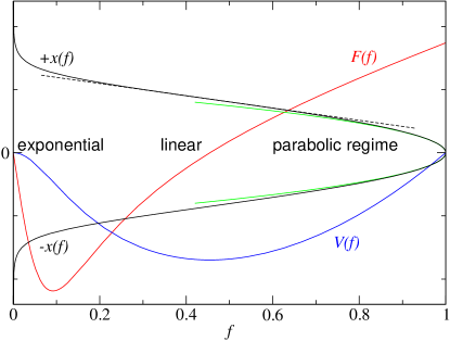
Figure 1: The typical form of functions $F(f)$ (2), $V(f)$ (5) and $x(f)$ (6) for a parameter value of $r=100$. Further, the different regimes are indicated according to the discussion in the introduction.

Further the integral (6) can be solved analytically for the limits $r\rightarrow 0$ (giving the Kerr soliton) and $r\rightarrow\infty$.

These partial analytical results, although being rather elementary, are not easily found in the literature and thus appear worth while mentioning in this article, see section II.1.

Apart from practical purposes it seems interesting that a power series solution of (6) can be obtained which allows, in principle, an arbitrarily exact calculation of soliton profiles independent of the intrinsic errors of numerical integration. However, the terms of this series are of increasing complexity and we do not prove the series’ convergence.

The article is organized as follows: In section II we resume the partial analytical results mentioned above, including the asymptotic solutions for $r\rightarrow 0$ and $r\rightarrow\infty$. Section III presents exact upper and lower bounds for the half width $\operatorname{hw}(r)$ which are rather close, especially for $r>1$. Section IV contains an outline of the approximation devised by Montemezzani and Günter Montemezzani and Günter (1997) as well as two new analytical approximations of $f(x)$ and the implied approximations of $\operatorname{hw}(r)$ which are of limited accuracy but relatively simple. The first one, called $V$-approximation, approximates the potential $V(f)$ by a cubic polynomial in $f^{2}$ such that the integral (6) can be done. The second one approximates the integrand $1/\sqrt{|V(f)|}$ of (6) by splitting off the two poles at $f=0$ and $f=1$ and replacing the remaining function $R(f)$ by the constant $R(1/2)$. It will be called “$I$-approximation”. Both methods give reasonable approximations of $\operatorname{hw}(r)$ which suffice for practical purposes and can be considered as alternatives to the approximations devised in Ref. Montemezzani and Günter (1997).

In section IV.3.2 we complete the $I$-approximation by a Taylor expansion of $R(f)$ about the center $f=1/2$ and show some examples of approximate soliton profiles. The number of terms of the Taylor series which are needed to achieve a good approximation of $f(x)$ increases with $r$. The lengthy but explicit expressions of the general Taylor coefficients can be obtained via the Faà di Bruno formula and are given in the appendix.

It is obvious that our methods of approximation are not confined to the special form of the photorefractive nonlinearity in (2) but could also be applied to other nonlinear Schrödinger equations or nonlinear oscillation problems.

II General properties and partial analytical results

II.1 General properties

The basic equation (1) is invariant under spatial reflections $x\mapsto x_{0}-x$ and translations into $x$-direction. Hence any solution $f(x)$ satisfying the (symmetric) initial conditions (3) is necessarily an even function of $x$, corresponding to the $\pm$ sign in (6). Since $V(f)<0$ for $0<f<1$, equation (4) shows that $f(x)$ is a strictly decreasing function for $x>0$.

The Taylor expansion of $f(x)$ about the centre $x=0$ starts with

$$f(x) =1-\frac{1}{2}V^{\prime}(1)x^{2}+\ldots$$

$$=1-\left(\frac{\ln(1+r)}{r}-\frac{1}{1+r}\right)x^{2}+\ldots$$ (8)

The corresponding parabola $f_{q}(x)=1-\frac{1}{2}{V^{\prime}}(1)x^{2}$ represents a lower bound of $f(x)$ since it has the maximal negative curvature of $f(x)$. Hence also its half width $\operatorname{hw}_{q}(r)$ will be a lower bound of $\operatorname{hw}(r)$:

$$\operatorname{hw}_{q}(r)=\sqrt{\frac{2(2-\sqrt{2})r(1+r)}{(1+r)\ln(1+r)-r}}<\operatorname{hw}(r)\quad.$$ (9)

Moreover, $\operatorname{hw}_{q}$ yields the qualitatively correct behaviour for $r\ll 1$ and $r\gg 1$:

$$\operatorname{hw}_{q}(r)\approx 2\sqrt{\frac{2-\sqrt{2}}{r}}\approx 1.53\frac{1}{\sqrt{r}}\quad(r\ll 1)$$ (10a)

$$\operatorname{hw}_{q}(r)\approx 2\sqrt{\left(1-\frac{1}{\sqrt{2}}\right)\frac{r}{\ln r}}\approx 1.08\sqrt{\frac{r}{\ln r}}\quad(r\gg 1)$$ (10b)

This has to be compared with the asymptotic expressions for $\operatorname{hw}(r)$, see below.

For $f\ll 1$ equation (1) assumes the asymptotic form

$$f_{xx}+V^{\prime\prime}(0)f=f_{xx}+2f\left(\frac{\ln(1+r)}{r}-1\right)=0$$ (11)

which has the solution

$$f(x)=C\exp\left(-\sqrt{|V^{\prime\prime}(0)|}x\right),\quad|x|\rightarrow\infty.$$ (12)

Hence all solitons considered show an asymptotic exponential decay for $|x|\rightarrow\infty$, the decay constant being a simple function of $r$.

II.2 Asymptotics for $r\rightarrow 0$

If $r\ll 1$, equation (1) assumes the asymptotic form

$${f^{\prime\prime}}-rf(1-2f^{2})=0$$ (13)

which is known from the cubic Schrödinger equation and has the soliton solution

$$f_{0}(x)=\mbox{sech}(\sqrt{r}x)\quad.$$ (14)

For the convergence of $f(x)$ towards the asymptotic form (14) see figure 2.

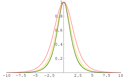
Figure 2: Numerically determined soliton profiles for small values of $r$. If the $x$-axis is scaled with $\sqrt{r}$ they converge to the sech$(x)$ solution. The chosen values are $r=10^{z}$ with $z=0,-1/2,-1,-3/2$.

The corresponding half width is

$$\operatorname{hw}_{0}=2\frac{1}{\sqrt{r}}{\rm arcosh}\sqrt{2}\approx\frac{1.76}{\sqrt{r}}\quad.$$ (15)

II.3 Asymptotics for $r\rightarrow\infty$

If $r\gg 1$ and $f^{2}\ln r\gg 1$, (1) assumes the asymptotic form of an oscillator equation

$${f^{\prime\prime}}+2\frac{\ln r}{r}f=0$$ (16)

with the solution

$$f_{\infty}(x)=\begin{cases}\cos\left(\sqrt{2\frac{\ln r}{r}}x\right)&|x|\leq\frac{\pi}{2}\sqrt{\frac{r}{2\ln r}}\\ 0&|x|>\frac{\pi}{2}\sqrt{\frac{r}{2\ln r}}\;.\end{cases}$$ (17)

Here we have taken into account that for small $f$, $f^{2}\ln r\gg 1$ as well as the approximation (16) will be no longer valid and the exponential decay will set in. In (17) this exponential decay is approximated by setting $f_{\infty}(x)=0$ for $|x|>\frac{\pi}{2}\sqrt{\frac{r}{2\ln r}}$. The approach of the exact solution $f(x)$ to (17) for $r\rightarrow\infty$ is much slower than for the analogous case $r\rightarrow 0$, see figure 3. For a similar result see Chen (1991).

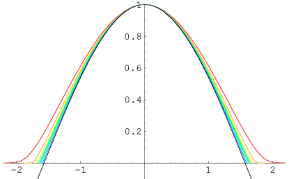
Figure 3: Numerically determined soliton profiles for large values of $r$. If the $x$-axis is scaled with $\sqrt{\frac{2\ln r}{r}}$ they converge slowly to the $\cos(x)$ solution. The chosen values are $r=10^{z}$ with $z=3,5,\ldots,15,30$.

The corresponding half width is

$$\operatorname{hw}_{\infty}=\sqrt{\frac{r}{2\ln r}}2\arccos\frac{1}{\sqrt{2}}\approx 1.11\sqrt{\frac{r}{\ln r}}.$$ (18)

III Exact bounds for the half width

We will utilise some properties of the (negative) force function $F(f)$ introduced in (2) which can be easily proven. It has a zero at

$$f_{0}=\sqrt{\frac{r-\ln(1+r)}{r\ln(1+r)}}<\frac{1}{\sqrt{2}}$$ (19)

which corresponds to the point of inflection $x(f_{0})$ of the soliton profile $f(x)$. It follows that the half width is attained before the point of inflection is reached, i. e.

$$\operatorname{hw}(r)<x(f_{0})\quad.$$ (20)

The second derivative of $F(f)$ with respect to $f$ vanishes at

$$f_{w}=\sqrt{\frac{3}{r}}\quad.$$ (21)

Some simple calculations then show that $F$ is a convex function within the physical domain $f\in[0,1]$ if $r<3$ and a concave function within the domain $f\in[f_{0},1]$ if $r>r_{0}\approx 9.3467$. Here $r_{0}$ is the solution of $f_{0}(r)=f_{w}(r)$. In both cases $F$ can be bounded by affine functions of the form $a(f)=m(f-1)+F(1)$. Note that an affine force function of this form would lead to harmonic oscillations $f(x)$ and a corresponding half width

$$\operatorname{hw}_{m}=\frac{2}{\sqrt{m}}\arccos\left(1-\frac{m}{F(1)}\left(1-\frac{1}{\sqrt{2}}\right)\right)\quad.$$ (22)

Now assume an inequality between two force functions $F_{1}<F_{2}$ within some domain. By integration we conclude $|V_{1}|<|V_{2}|$ and, using (6), the reverse inequality $x_{2}(f)<x_{1}(f)$ for the positive branch $x_{i}(f)>0,\;i=1,2$. Hence also $\operatorname{hw}_{2}<\operatorname{hw}_{1}$ if the half width is assumed within the domain under consideration.

By applying these arguments to our particular cases we obtain

$$s(f)>F(f)>t(f)\qquad\forall f\in(0,1)\qquad(r<3)$$ (23)

where $t=t(f)$ is the tangent through the point $(1,F(1))$,

$$t(f)=m_{t}(f-1)+F(1),\;\text{with}$$ (24a)

$$m_{t}\equiv\left.\frac{\partial F}{\partial f}\right|_{f=1}=F(1)+\frac{4r}{(1+r)^{2}},$$ (24b)

and $s(f)$ is the secant through $(1,F(1))$ and $(f_{0},F(f_{0}))$,

$$s(f)=m_{s}(f-1)+F(1),\qquad m_{s}\equiv\frac{F(1)}{1-f_{0}}.$$ (25)

Consequently,

$$\operatorname{hw}_{m_{s}}<\operatorname{hw}<\operatorname{hw}_{m_{t}}\qquad(r<3)\quad.$$ (26)

In the case of $F$ being concave the inequalities (23) and (26) are just inverted and we obtain

$$\operatorname{hw}_{m_{t}}<\operatorname{hw}<\operatorname{hw}_{m_{s}}\qquad(r>r_{0}\approx 9.3467)$$ (27)

Fig. 4 confirms in a double-logarithmic plot that the numerically determined half width lies between $\operatorname{hw}_{m_{s}}$ and $\operatorname{hw}_{m_{t}}$. For $r>10$ the two bounds almost coincide.

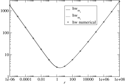
Figure 4: Exact bounds $\operatorname{hw}_{m_{s}}$, $\operatorname{hw}_{m_{t}}$ for the half width according to (22), (24b), (25) and the numerically determined half width as functions of $r$.

IV Analytical approximations of the soliton profile

As explained in the introduction it would be desirable to have analytical approximations of the soliton profile $f(x)$ and half width $\operatorname{hw}(r)$ which are not too complex in form and yet give qualitatively correct results for a large range of values of $r>0$. In this section we will present the three approximations mentioned in the introduction.

IV.1 P-approximation, cf. Montemezzani and Günter (1997)

We will call the approximation of the soliton profile $f(x)$ due to G. Montemezzani and P. Günter “P-approximation”. It will suffice to briefly sketch it and to refer the reader for more details to Montemezzani and Günter (1997).

The key idea is to expand the inverse soliton profile $1/f(x)$ into an even power series $P(x)=\sum_{n=0}^{\infty}a_{2n}x^{2n}$. Inserting this ansatz into (1) allows the determination of arbitrary coefficients $a_{2n}$ by means of recursion relations. Hence this method yields, in principle, arbitrary precise approximations of $f(x)$.

However, there are – to our opinion – some minor disadvantages of the P-approximation which motivate the development of alternative approximations:

• For concrete approximations $P(x)$ has to be replaced by a polynomial of degree, say, $2n$. In this case the exponential decay of $f(x)$ is not properly reproduced.

• The half-width $\operatorname{hw}(r)$ can be given by an explicit expression only for $n\leq 4$, in simple form even only for $n=2$, see Montemezzani and Günter (1997).

• We do not see any possibility to extend the P-approximation to the case of dark solitons, in contrast to the according claim in Montemezzani and Günter (1997).

IV.2 $V$-approximation

The $V$-approximation is an approximation of $V(f)$ in the neighbourhood of $f=1$ which reproduces the zeros of $V$ (the double zero $f=0$ and the simple zero $f=1$):

Introducing the abbreviation

$$\varphi(u)\equiv\frac{\ln(1+u)}{u}\quad,$$ (28)

the potential $V$ can be written as

$$V(f)=f^{2}\left(\varphi(r)-\varphi(rf^{2})\right)\quad.$$ (29)

A Taylor series of $\varphi$ with the centre $f=1$ including terms of second order $(1-f)^{2}$ yields the approximation

$$V_{0}(f)=-\frac{1}{8}\alpha f^{2}\left(f^{2}-1\right)\left(f^{2}-f_{1}^{2}\right)$$ (30)

where

$$f_{1}^{2}\equiv\frac{-5r^{2}-4r+4(1+r)^{2}\ln(1+r)}{-3r^{2}-2r+2(1+r)^{2}\ln(1+r)}$$ (31)

and

$$\alpha\equiv 4\frac{-3r^{2}-2r+2(1+r)^{2}\ln(1+r)}{r(1+r)^{2}}\quad.$$ (32)

By inserting the approximated potential $V_{0}$ into equation (6) and solving the integral we obtain the approximated soliton intensity

$$f_{V}^{2}(x)=\frac{2f_{1}^{2}}{f_{1}^{2}+\left(f_{1}^{2}-1\right)\cosh\left(\sqrt{\alpha}f_{1}x\right)}$$ (33)

and the half width

$$\operatorname{hw}_{V}(r)=2\frac{1}{\sqrt{\alpha}f_{1}}\operatorname{arcosh}\frac{3f_{1}^{2}-1}{f_{1}^{2}-1}\quad.$$ (34)

Due to the choice of the centre $f=1$ in the Taylor approximation the soliton profile is well approximated in the neighbourhood of the maximum $f=1$ for all $r>0$. In fact, plots of $f(x)$ for different $r$ show a good agreement of $f_{V}$ and $f$ if $\frac{1}{\sqrt{2}}\leq f\leq 1$ for arbitrary $r$. This can be explained by a comparison with the $r\rightarrow 0$ approximation $f_{0}(x)=\mbox{sech}(\sqrt{r}x)$ which yields the result

$$\frac{f_{V}(x)}{f_{0}(x)}=1+\frac{2}{3}x^{2}r^{2}+{\cal O}(x^{2}r^{3}).$$ (35)

Therefore we expect to find a good approximation of the soliton’s half width for all $r$. Indeed, if $r\ll 1$, the result of the $r\rightarrow 0$ approximation (15) of the half width is reproduced exactly:

$$\operatorname{hw}_{V}(r)=\frac{2}{\sqrt{r}}\left(\operatorname{arcosh}\sqrt{2}+{\cal O}(r)\right)=\operatorname{hw}_{0}(r)+{\cal O}(\sqrt{r}).$$ (36)

For large values of $r$, we find

$$\operatorname{hw}_{V}(r) \approx\sqrt{\frac{r}{\ln(r)}}\frac{\ln(5+2\sqrt{6})}{2}$$

$$\approx 1.1462\sqrt{\frac{r}{\ln(r)}}\qquad(r\gg 1),$$ (37)

which does not reproduce the result (18) exactly, but yields a good approximation.

On the other hand, the soliton profile $f(x)$ in the region $f\ll 1$ is only reproduced if $r\ll 1$, thus the $V$-approximation is not suited to analyse the exponential decrease.

IV.3 $I$-approximation

According to (6) the soliton’s shape is not directly governed by the potential $V$ but by the integrand

$$I(f)\equiv\frac{1}{\sqrt{-V(f)}}.$$ (38)

Hence, an approximation of the integrand rather than the potential itself might be a good starting point for approximating the soliton, too. Taking into account the poles at $f=1$ and $f=0$ it is a natural idea to split the integrand up into three distinct parts as

$$\frac{1}{\sqrt{-V(f)}}=\frac{c_{1}}{f}+\frac{c_{2}}{\sqrt{1-f}}+R(f),$$ (39)

where a new function $R(f)$ and the two constants $c_{1}$ and $c_{2}$ have been introduced. The constants can be determined by

$$c_{1} \equiv\lim_{f\to 0}\frac{f}{\sqrt{-V(f)}}=\frac{1}{\sqrt{-\frac{1}{2}{V^{\prime\prime}}(0)}}$$

$$=\left[\left(1-\frac{\ln(1+r)}{r}\right)\right]^{-\frac{1}{2}}$$ (40)

and

$$c_{2} \equiv\lim_{f\to 1}\frac{\sqrt{1-f}}{\sqrt{-V(f)}}=\frac{1}{\sqrt{{V^{\prime}}(1)}}$$

$$=\left[2\left(\frac{\ln(1+r)}{r}-\frac{1}{1+r}\right)\right]^{-\frac{1}{2}}.$$ (41)

While the integrand’s behaviour at the poles is correctly covered by the first two summands of (39) the function $R(f)$ dominates the integrand in the region between the poles. A good approximation of the integrand can now be achieved by expanding the function $R(f)$ into a Taylor series. Due to its construction this fits the exact soliton best for $f\approx 1$ and $f\ll 1$.

IV.3.1 $0^{\text{th}}$ order $I$-approximation

Since $R(f)$ does not vary too much over the interval $0<f<1$ even a $0^{\text{th}}$ order approximation yields good results. $R(f)$ will be expanded around $f=1/2$. Note that this choice is rather arbitrary but seems reasonable. Up to order 0 the $I$-approximation gives

$$I(f)\approx\frac{c_{1}}{f}+\frac{c_{2}}{\sqrt{1-f}}+c_{3},$$ (42)

with

$$c_{3}\equiv R\left(\frac{1}{2}\right)\\ =\frac{2\sqrt{r}}{\sqrt{4\ln(4+r)-\ln(1+r)-8\ln 2}}-2c_{1}-\sqrt{2}c_{2}\;.$$ (43)

By a simple integration one obtains

$$-c_{1}\ln f+2c_{2}\sqrt{1-f}+c_{3}(1-f)=\sqrt{2}x,$$ (44)

and the corresponding half width

$$\operatorname{hw}_{I}(r)=\sqrt{2}\left(c_{1}(r)\ln\sqrt{2}+2\sqrt{1-\frac{1}{\sqrt{2}}}\;c_{2}(r)\right.\\ +\left.\left(1-\frac{1}{\sqrt{2}}\right)c_{3}(r)\right).$$ (45)

For small $r$ a series expansion with respect to $r$ yields

$$\operatorname{hw}_{I}(r)\approx\frac{1.82}{\sqrt{r}}\qquad(r\ll 1).$$ (46)

Although the result of the low amplitude approximation (15) is not reproduced exactly, this is in fact very close to it.

For large values of $r$ we find

$$\operatorname{hw}_{I}(r) \approx\sqrt{\frac{r}{2\ln r}}2\left[\sqrt{2-\sqrt{2}}\;+\right.$$

$$\quad\left.\left(1-\frac{1}{\sqrt{2}}\right)\left(\frac{2}{\sqrt{3}}-1\right)\right]$$ (47)

$$\approx 1.1465\sqrt{\frac{r}{\ln(r)}}\qquad(r\gg 1),$$ (48)

which matches the corresponding value of the V-approximation up to three decimal places.

Finally, for $f\ll 1$, from eq. (44) one easily derives the exponential decrease of the soliton:

$$f(x)\approx\exp\biggl{(}{\frac{2c_{2}+c_{3}-\sqrt{2}x}{c_{1}}}\biggr{)}\qquad(f\ll 1).$$ (49)

Fig. 5 shows that the approximated half width $\operatorname{hw}_{V}$ and $\operatorname{hw}_{I}$ are in good agreement with the numerically determined half width.

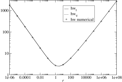
Figure 5: Approximated half widths $\operatorname{hw}_{V}$, $\operatorname{hw}_{I}$ according to (34), (45) and the numerically determined half width as functions of $r$ – almost indistinguishable.

The shape of the soliton is very well fitted by the $0^{\text{th}}$ order $I$-approximation as well, see Fig. 6

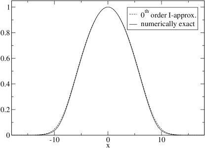
Figure 6: $0^{\text{th}}$ order $I$-approximation and numerically exact soliton, $r=100$.

IV.3.2 Higher order $I$-approximations

Although for practical purposes the $0^{\text{th}}$ order $I$-approximation gives a sufficiently accurate approximation of the half width, the shape of the soliton has still room for improvement, especially for large $r$. The necessary enhancement of the $I$-approximation can easily be achieved by taking higher order Taylor coefficients into account. Fig. 7 shows that even for very large $r$ a satisfactory approximation can be achieved with a second order $I$-approximation. If still higher order approximations are needed the necessary Taylor coefficients are given in Appendix A.

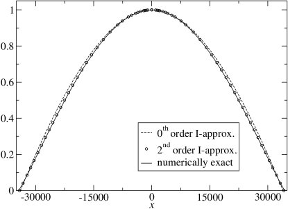
Figure 7: $0^{\text{th}}$ and $2^{\text{nd}}$ order $I$-approximation together with the numerically exact soliton for $r=10^{10}$.

V Summary

In this paper we considered the profile $f(x)$ of spatial one-dimensional bright photorefractive solitons, depending on an intensity parameter $r>0$, which is only given by means of an integral (6) but not in closed form.

We presented partial analytical results which allow a semi-quantitative discussion of the profile and studied the closed form solutions for the limit cases $r\rightarrow 0$ and $r\rightarrow\infty$. We also provided exact bounds of the half width curve $\operatorname{hw}(r)$.

Moreover, we devised several analytical approximations of the soliton profile and the half width which are relatively simple in form, but in excellent agreement with the numerical results. These approximations would thus suffice for the practical purpose of comparing experimental data with theoretical descriptions. If an arbitrary high accuracy of the approximation is desired one has to resort to the Taylor series (67). Altogether, we thus consider the problem of evaluating the soliton profile (6) as essentially solved.

We expect that our methods can be used as a basis to analyse more complex situations such as photorefractive solitons under influence of diffusion and also be transferred to the problem of dark and grey solitons.

Appendix A Taylor coefficients of $R(f)$

In order to give the explicit expression of the Taylor coefficients of the integrand $I(f)$ and the rest function $R(f)$ we write them as the composition of auxiliary functions that can be handled much better. Let

$$g_{1}(x)=\ln(1+rx^{2}),g_{2}(x)=x^{2}\ln(1+r),$$ (50)

$$g(x)=g_{1}(x)-g_{2}(x),\;\text{and}$$ (51)

$$h(x)=\frac{1}{\sqrt{x}}.$$ (52)

Then the integrand $I$ can be rewritten as

$$I(f)=\sqrt{r}\cdot[h\circ g](f)$$ (53)

The $n$th derivative of all the constituents of $I(f)$ can easily be calculated. For $n\geq 1$ they read

$$g_{2}^{(1)}(x)=2x\ln(1+r),\quad g_{2}^{(2)}(x)=2\ln(1+r),$$ (54)

$$n>2:\,g_{2}^{(n)}(x)=0,$$ (55)

$$g^{(n)}(x)=g_{1}^{(n)}(x)-g_{2}^{(n)}(x),$$ (56)

$$h^{(n)}(x)=2\cdot\left(-\frac{1}{4}\right)^{n}\frac{(2n-1)!}{(n-1)!}\cdot x^{-\frac{2n+1}{2}},$$ (57)

and

$$g_{1}^{(n)}(x)=\sum_{k=\lceil\frac{n}{2}\rceil}^{n}\frac{(-1)^{k+1}r^{k}n!}{(1+rx^{2})^{k}k}\binom{k}{n-k}(2x)^{2k-n},$$ (58)

where $\lceil n/2\rceil$ means the smallest integer greater than or equal to $n/2$. The $n$th derivative of the integrand can now be determined using the Faà di Bruno formula (cf. Constantine and Savits (1996) and Aldrovandi (2001)):

$$I^{(n)}(x)=\sqrt{r}\cdot\sum_{k=1}^{n}h^{(k)}(g(x))\cdot\\ \mathbb{B}_{nk}(g^{(1)}(x),g^{(2)}(x),\dots,g^{(n-k+1)}(x)).$$ (59)

The Bell matrices $\mathbb{B}_{nk}$ used in this formula are defined by

$$\mathbb{B}_{nk}(z_{1},z_{2},\dots,z_{n-k+1})=\\ \sum_{\{\nu_{i}\}}\frac{n!}{\prod_{j=1}^{n}[\nu_{j}!(j!)^{\nu_{j}}]}z_{1}^{\nu_{1}}z_{2}^{\nu_{2}}\dots z_{n-k+1}^{\nu_{n-k+1}},$$ (60)

where the sum is taken over all those sets $\{\nu_{i}\}$ of non-negative integers which satisfy

$$\sum_{j=1}^{n}j\nu_{j}=n\quad\text{and}\quad\sum_{j=1}^{n}\nu_{j}=k.$$ (61)

To proceed we again define two auxiliary functions

$$g_{3}(x)=\frac{c_{1}}{x}\quad\text{and}\quad g_{4}(x)=\frac{c_{2}}{\sqrt{1-x}},$$ (62)

such that

$$R(f)=I(f)-g_{3}(f)-g_{4}(f).$$ (63)

With the derivatives

$$g_{3}^{(n)}(x)=c_{1}\,(-1)^{n}\,n!\,x^{-(n+1)}\quad\text{and}$$ (64)

$$g_{4}^{(n)}(x)=8c_{2}\cdot\left(\frac{1}{4}\right)^{n+1}\frac{(2n-1)!}{(n-1)!}\cdot(1-x)^{-\frac{2n+1}{2}}$$ (65)

we can calculate the $n$th derivative of $R(f)$ as

$$R^{(n)}(f)=I^{(n)}(f)-g_{3}^{(n)}(f)-g_{4}^{(n)}(f).$$ (66)

The final result then reads

$$\pm\sqrt{2}x(f)=c_{1}\ln f-2c_{2}\sqrt{1-f}\\ +\sum_{n=0}^{\infty}R^{(n+1)}\left(\frac{1}{2}\right)\frac{(f-\frac{1}{2})^{n+1}-(\frac{1}{2})^{n+1}}{(n+1)!}\;.$$ (67)

Although for practical purposes it is much easier to calculate higher derivatives of $R(f)$ by some computer algebra system it is nevertheless interesting that they can indeed be given explicitly. Convergence issues of the respective Taylor series have not been considered here.

References

- Segev et al. (1992) M. Segev, B. Crosignani, A. Yariv, and B. Fischer, Phys. Rev. Lett. 68, 923 (1992).
- Segev et al. (1994) M. Segev, G. C. Valley, B. Crosignani, P. DiPorto, and A. Yariv, Phys. Rev. Lett. 73, 3211 (1994).
- Duree et al. (1993) G. C. Duree, J. L. Shultz, G. J. Salamo, M. Segev, A. Yariv, B. Crosignani, P. DiPorto, E. J. Sharp, and R. R. Neurgaonkar, Phys. Rev. Lett. 71, 533 (1993).
- Segev et al. (1996) M. Segev, M. Shih, and G. Valley, J. Opt. Soc. Am. B 13, 706 (1996).
- Montemezzani and Günter (1997) G. Montemezzani and P. Günter, Opt. Lett. 22, 451 (1997).
- Christodoulides and Carvalho (1995) D. Christodoulides and M. Carvalho, J. Opt. Soc. Am. B 12, 1628 (1995).
- Meng et al. (1997) H. Meng, G. Salamo, F. Shih, and M. Segev, Opt. Lett. 22, 448 (1997).
- Kos et al. (1998) K. Kos, G. Salamo, and M. Segev, Opt. Lett. 23, 1001 (1998).
- Wesner et al. (2001) M. Wesner, C. Herden, D. Kip, E. Krätzig, and P. Moretti, Opt. Commun. 188, 69 (2001).
- Wesner (2003) M. Wesner, Nichtlineare optische Effekte im Ferroelektrikum Strontiumbariumniobat (Cuvillier Verlag Göttingen, 2003).
- Chen (1991) Y. Chen, Opt. Lett. 16, 4 (1991).
- Constantine and Savits (1996) G. M. Constantine and T. H. Savits, T. Am. Math. Soc. 348, 503 (1996).
- Aldrovandi (2001) R. Aldrovandi, Special Matrices of Mathematical Physics (World Scientific Publishing, 2001).