Understanding visual map formation through vortex dynamics
of spin Hamiltonian models

Abstract

The pattern formation in orientation and ocular dominance columns is one of the most investigated problems in the brain. From a known cortical structure, we build spin-like Hamiltonian models with long-range interactions of the Mexican hat type. These Hamiltonian models allow a coherent interpretation of the diverse phenomena in the visual map formation with the help of relaxation dynamics of spin systems. In particular, we explain various phenomena of self-organization in orientation and ocular dominance map formation including the pinwheel annihilation and its dependency on the columnar wave vector and boundary conditions.

A series of experiments have suggested that important elements of the organization of ocular dominance (OD) and orientation preference (OP) maps in the striate cortex are not prespecified but emergent during an activity-driven, self-organizing process Hubel and Wiesel (1977); LeVay et al. (1978); Stryker et al. (1978). An optical imaging technique Blasdel (1992); Blasdel and Salama (1986); Grinvald et al. (1986) revealed the detailed maps of OD and OP over small patches of the cortex, which prompted several models for the map generation in the brain and various attempts for the analysis of the properties in the observed cortical map patterns Erwin et al. (1995); Swindale (1996).

In the experimentally observed OP columnar patterns, there are two prominent features: (1) singular points (so called “pinwheels”) are point-like discontinuities around which the orientation preference changes by multiples of 180^∘ along a closed loop, and (2) linear zones are regions where iso-orientation contours (IOCs) are straight and run in parallel for a considerable distance Swindale et al. (1987); Bonhoeffer and Grinvald (1991); Maldonado et al. (1997). The analysis of competitive Hebbian models Obermayer et al. (1992); Durbin and Mitchison (1990) predicted the bifurcation between homogeneous and inhomogeneous solutions depending on the cooperation range $\sigma$ and the change in the wavelength $\Lambda$ Hoffsümmer et al. (1995); Scherf et al. (1999); Goodhill and Cimponeriu (2000). Linear zones in OP columns or OD bands are features of the inhomogeneous states. Some experimental or simulational results suggested that pinwheels are not permanent structures but can be annihilated during the course of active-dependent development Wolf and Geisel (1998); Daw (1998). The perpendicular intersection of IOCs and OD bands with the margin of the striate cortex has been also reported Obermayer and Blasdel (1993); LeVay et al. (1985). There are some evidence that patterns in OP and OD columns are not independent but correlated. Pinwheels have a tendency to align with the centers of OD bands and IOCs intersect the borders of OD bands at a steep angle Obermayer and Blasdel (1993). The influence of the interactions between OP and OD columns on the pinwheel stability was described Wolf and Geisel (1998).

In this paper, we propose a new visual map formation method with neighborhood interactions. The cortical map generation is described by spin-like Hamiltonians with distance dependent interactions. The statistical analysis of these Hamiltonians leads to the successful description of several pattern properties observed in vivo. In our analogy, the progress in the visual map formation corresponds to relaxation dynamics in spin systems, where, for example, the pinwheels in OP can be regarded as (in-plane) vortices. The pinwheel instability and its annihilation rate are explained in terms of the free energy of the topological excitation or the Kosterlitz and Thouless transition temperature Kosterlitz and Thouless (1973). Our model with neighborhood interaction exhibits the bifurcation between the homogeneous and inhomogeneous states depending on the inhibitory activity strength $k$ in lateral currents. The columnar wavelength and the correlation function of the OP maps are also derived from out model. The extension of our model to the $O(3)$ or the Heisenberg model induces the correlation between the OP and OD columns, which leads to the orthogonality between IOCs and the borders of OD bands, and allows OD columns to influence on the pinwheel stability. Another orthogonal tendency of the cortical maps with area boundaries is explained from the equilibrium condition.

The six layers in the neocortex can be classified into three different functional types. The layer IV neurons first get the long range input currents, such as signals from the retina via the lateral geniculate nucleus (LGN) of the thalamus, and send them up vertically to layer II and III that are called the true association cortex. Output signals are sent down to the layer V and VI, and sent further to the thalamus or other deep and distant neural structures. Lateral connections also occur in the superficial (layer II and III) pyramidal neurons and have usual antagonistic propensity which sharpens responsiveness to an area. However, the superficial pyramidal neurons also send excitatory recurrent to adjacent neurons due to unmyelinated collaterals. Horizontal or lateral connections have such distance dependent (so called ”Mexican hat” shaped) excitatory or inhibitory activity. Some bunches of neurons make columnar clusters called minicolumns and such aggregations are needed to consider higher dimensional properties of processing elements Calvin (1998); Lund et al. (1998).

Now we propose a Lie algebraic representation method for the feature vectors in cortical maps, called the fibre bundle map (FBM) model. This starts from the assumption that the total space $E$ is composed of the lattice (or base) space $B$ and the pattern (or fibre) space $F$. A transition function (or symmetry) group $G$ of a homeomorphism of the fibre space $F$ is necessary to describe what happens if there is “excitatory” or “inhibitory” activity. The symmetry group $G$ is important since it determines what interactions are possible. In the visual cortex, $G$ takes $O(3)$ rather than $O(2)\times Z_{2}$ because of the correlations between OP and OD columns.

If there are stimuli from lateral and LGN neurons in the OP columns, the changes in preferred angles $\phi_{i}$ ($0\leq\phi_{i}<\pi)$ for $i$-th neuron group are described by

$$\frac{\partial\phi_{i}}{\partial t} = -2\varepsilon\sum_{j}I({\vec{r}}_{i},{\vec{r}}_{j})\sin(2\phi_{i}-2\phi_{j})$$ (1)

$$-2\mu B_{i}\sin(2\phi_{i}-2\phi_{i}^{\prime}),$$

where $\varepsilon$ and $\mu$ are the change rates in the stimuli from lateral and LGN cells, respectively, and $B$ and $\phi^{\prime}$ are the strength and the phase of LGN stimulus. We use the lateral neighborhood interaction function $I$, modified from a wavelet, as

$$I_{WL}({\vec{r}}_{i},{\vec{r}}_{j})=\left(1-k\frac{|{\vec{r}}_{i}-{\vec{r}}_{j}|^{2}}{\sigma^{2}}\right)\exp(-\frac{|{\vec{r}}_{i}-{\vec{r}}_{j}|^{2}}{2\sigma^{2}}).$$ (2)

Note that there is also another well-known Mexican hat shaped function called the difference of Gaussians (DOG) filter, $I_{DOG}(r)=\exp(-r^{2}/2\sigma_{1}^{2})-k\exp(-r^{2}/2\sigma_{2}^{2})$. We rewrite Eq. (1) as a gradient flow with the Hamiltonian

$$H = -\sum_{i,j}J({\vec{r}}_{i},{\vec{r}}_{j}){\bf S}_{i}\cdot{\bf S}_{j}-\sum_{i}{\bf h}_{i}\cdot{\bf S}_{i},$$ (3)

where $J({\vec{r}}_{i},{\vec{r}}_{j})=\frac{\varepsilon}{2}I({\vec{r}}_{i},{\vec{r}}_{j})$ is site distance dependent interaction energy. The site states ${\bf S}_{i}=(\cos 2\phi_{i},\sin 2\phi_{i})$ and the external stimuli ${\bf h}_{i}=(\mu B_{i}\cos 2\phi_{i}^{\prime},\mu B_{i}\sin 2\phi_{i}^{\prime})$ are 2-components vectors. In this form, $H$ is similar to spin models in statistical physics. In the case of OD maps, ${\bf S}_{i}$ has a one-component with $\pm 1$ values similar to the Ising model. There were some previous studies on spin models with distance dependent interactions, albeit mostly in the form of $J(r)\sim r^{-\alpha}$  Monroe et al. (1990); Luijten and Blöte (1997); Krech and Luijten (2000); Ifti et al. (2001).

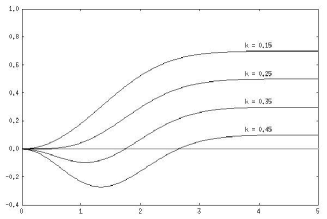
$q$

${\tilde{J}}(0)-{\tilde{J}}(q)$

Figure 1: The plot of ${\tilde{J}}(0)-{\tilde{J}}(q)$ vs $q$ in Eq. (5). For $k>k_{c}$ (=$1/4$), the minimum point at $q^{\ast}=0$ becomes unstable.

The Hamiltonian in Eq.(3) can be easily diagonalized in the momentum space:

$$H=-\sum_{\vec{q}}{\tilde{J}}({\vec{q}}){\bf S}_{\vec{q}}\cdot{\bf S}_{-{\vec{q}}}-\sum_{\vec{q}}{\bf h}_{\vec{q}}\cdot{\bf S}_{-{\vec{q}}},$$ (4)

where ${\tilde{J}}({\vec{q}})=\sum_{\vec{r}}J({\vec{r}})e^{-i{{\vec{q}}\cdot{\vec{r}}}}$, ${\bf S}_{\vec{q}}=\frac{1}{\sqrt{N}}\sum_{i}{\bf S}_{i}e^{-i{{\vec{q}}\cdot{\vec{r}}}_{i}}$ and ${\bf h}_{\vec{q}}=\frac{1}{\sqrt{N}}\sum_{i}{\bf h}_{i}e^{-i{{\vec{q}}\cdot{\vec{r}}}_{i}}$. We assume that the LGN stimuli for a given neuron is uniform with no preferred angle, so that the second term in Eq. (3) is neglected without random fluctuations effect. In the continum limit, we obtain

$${\tilde{J}}({\vec{q}})\simeq\pi\varepsilon\frac{\sigma^{2}}{a^{2}}(1-2k+k\sigma^{2}q^{2})e^{-\sigma^{2}q^{2}/2},$$ (5)

where $a$ is the lattice constant. ${\tilde{J}}({\vec{q}})$ has the maximum at $q^{\ast}=0$ for $k<k_{c}$ (=1/4) and at $q^{\ast}=\frac{1}{\sigma}\sqrt{4-1/k}$ for $k>k_{c}$ (Fig. 1). Therefore, there is a threshold depending on $k_{c}$ below which OP slabs or OD bands are forbidden. Above $k_{c}$, columnar patterns emerge with the wavelength $\Lambda=2\pi/q^{\ast}$, which decreases as $k$ increases (Fig. 2 (b) and (c)).

In the simulations of the OP map formation starting from a random state by Eq. (1), dense pinwheels first emerge with the spin-waves for $k<k_{c}$ (Fig. 2 (a)) as for the classical XY model. Then pinwheels start to annihilate in pairs and eventually the map approaches a homogeneous state. For $k>k_{c}$ (Fig. 2 (b) and (c)), pinwheels emerge with the columnar patterns and are annihilated in time as well. The OP map will eventually approach the equilibrium state that is composed of a uni-directional plane-wave, the winner in the competition among $|{\vec{q}}|=q^{\ast}$ states.

$t=5$

$t=15$

$t=100$

(a) $k=0.2$

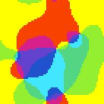
(b) $k=0.3$

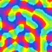
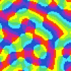
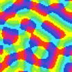
(c) $k=1.0$

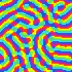
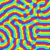
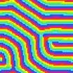
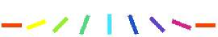
Figure 2: Simulation results of the OP map using Eq. (1). Maps are generated with $\sigma^{2}=6$, $\varepsilon=10^{-3}$, $\mu=0$, periodic boundary conditions and an initially random state in $70\times 70$ lattice.

By using the parabolic behavior of $-{\tilde{J}}(q)$ near the minimum point $q^{\ast}$, the Hamiltonian can be approximated as

$$H\simeq-\sum_{{\vec{q}}}\left[{\tilde{J}}(q^{\ast})+\frac{1}{2}{\tilde{J}}^{\prime\prime}(q^{\ast})|{\vec{q}}-{\vec{q}}^{\ast}|^{2}\right]{\bf S}_{{\vec{q}}}\cdot{\bf S}_{-{\vec{q}}}$$ (6)

or the effective Hamiltonian as a function of the preferred orentation $\phi$ is given by

$$H[\phi]\simeq-NJ_{s}+\frac{J_{p}}{2}\int d{\vec{r}}|2{\vec{\nabla}}\phi-{\vec{q}}^{\ast}|^{2},$$ (7)

where $J_{s}={\tilde{J}}(q^{\ast})$, $J_{p}=-{\tilde{J}}^{\prime\prime}(q^{\ast})/a^{2}$ ($=2\pi\varepsilon\frac{\sigma^{4}}{a^{4}}(4k-1)\exp(-2+1/2k)$ for $k>k_{c}$), and both $J_{s}$ and $J_{p}$ are positive for all $k$. The term ${\vec{q}}^{\ast}$ in Eq. (7), which makes plane-wave solutions, does not contribute to the pinwheel formation energy since ${\bf\nabla}\times{\bf\nabla}\phi_{pw}=0$ and the line integral around any contour vanishes by Stoke’s theorem. Just adapting the results in vortex dynamics Kosterlitz and Thouless (1973), we can obtain the change in free energy due to the formation of a pinwheel, $\Delta G=(\pi J_{p}-2k_{B}T)\ln(L/a)$, and the phase transition temperature, $T_{KT}=\pi J_{p}/2k_{B}$.

The visual cortex arises through activity-dependent refinement of initially unselective patterns of synaptic connections, whereas dense pinwheels emerge when orientation selectivity is first established and the density of pinwheels decreases by annihilation in time. The observed pinwheel densities differ in several species and such difference in the pinwheel annihilation rates has been discussed by Wolf et al. Wolf and Geisel (1998). Now we can predict the relative pinwheel annihilation rates in terms of $\Delta G$ or $T_{KT}$: (i) As $k$ increases for $k>k_{c}$, $J_{p}$ increases and the pinwheels become more unstable. For fixed $\varepsilon$ and $\sigma$, $\Lambda$ decreases as $k$ increases and the map with a narrower wavelength relaxes to the equilibrium state more rapidly (Fig. 2 (b) & (c)). (ii) As $\sigma$ increases, pinwheels become more unstable. But $\Lambda$ is proportional to $\sigma$, and the map with a narrower wavelength relaxes to the equilibrium state more slowly in this case. (iii) The parameter $\varepsilon$ can be regardes the activity rate responding to external stimuli or the learning rate due to the Hebbian rule. The annihilation rate becomes larger for larger $\varepsilon$. (iv) Thermal fluctuations may lead to the persistence of the pinwheel structure but they also disturb the map organization. (v) There are pinwheel annihilation mechanisms by collisions not only between opposite vortices but also with area boundaries. The probability of a collision with area boundaries decreases as the lattice size increases for randomly moving pinwheels. (vi) To include the interactions between OD and OP columns, our model has to be extended to the $O(3)$ symmetry or Heisenberg model. The classical anisotropic Heisenberg model is described by

$$H=-K\sum_{\langle ij\rangle}(S_{i}^{x}S_{j}^{x}+S_{i}^{y}S_{j}^{y}+\lambda S_{i}^{z}S_{j}^{z}),$$ (8)

where $K>0$. For this model, $T_{KT}$ is known to approach 0 as $\lambda$ approaches $1$ Hikami and Tsuneto (1980). This result can be translated as follows: the pinwheel structures last longer or even become stabilized through strong activity of OD column.

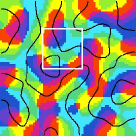
(a)

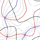
(b)

Figure 3: (a) An simulation result of OP and OD columnar patterns using Eq. (3) with ${\bf S}=(S_{x},S_{y},S_{z})$ and (b) its detailed contour feature in a white rectangle (non-periodic boundary conditions). The blue lines correspond to $S_{x}=0$ ($\phi=\frac{\pi}{4}$ or $\frac{3\pi}{4}$) domains and the red lines, $S_{y}=0$ ($\phi=0$ or $\frac{\pi}{2}$) domains. The black lines are the borders of opposite OD (or $S_{z}=0$) domains in both figures.

The extension to the Heisenberg model also explains the observed orthogonal property between the borders of OD bands and the IOCs. Let us consider the gradient or normal vectors of IOCs at $S_{x}=0$ and $S_{y}=0$. These two vectors intersect perpendicularly at pinwheels. The borders of the opposite OD domains can be represented as $S_{z}=0$, which will meet also perpendicularly with other contours, $S_{x}=0$ or $S_{y}=0$. Therefore, the borders of OD bands are mathematically equivalent to IOCs and intersect perpendicularly with each other (Fig. 3).

The correlation function in the OP maps is obtained from Eq. (7) as

$$\langle{\bf S}(r)\cdot{\bf S}(0)\rangle=g(r)\simeq J_{0}(q^{\ast}r)\ \left(\frac{r}{a}\right)^{-k_{B}T/2\pi J_{p}},$$ (9)

where $J_{0}$ is the zeroth Bessel function. As the map relaxes to the equilibrium state, the correlation function is expected to approach the distribution in Eq. (9). This is consistent with the experimens Erwin et al. (1995) and the numerical simulations (Fig. 5).

The perpendicularity with the margin of the striate cortex is derived from the equilibrium condition $\delta H/\delta\phi\sim 0$ or $\nabla^{2}\phi\sim 0$. The normal component of ${\bf\nabla}\phi$ vanishes at the area boundary since the integral along a narrow rectangular loop over the area boundary, $\oint_{C}{\bf\nabla}\phi\cdot d\vec{n}$, vanishes due to the divergence theorem. Such perpendicularity with the area boundary is also manifested in other static field solutions, such as the magnetic field, and is consistent with the observed OD patterns in vivo (Fig. 5).

$g(r)$

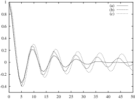
$r$

Figure 4: (a) Normalized autocorrelation function $g(r)$ of the simulation results in Fig. 2 (c) at $t=5$ and (b) $t=100$. (c) The zeroth Bessel function $J_{0}(q^{\ast}r)$.

Figure 5: The complete pattern of OD stripes in the striate cortex of a macaque monkey. There is a strong tendency for the stripes to meet the margin of striate cortex at steep or right angles (LeVay LeVay et al. (1985), Copyright 1985 by the Society for Neuroscience).

The interactions in cortical circuitry and the synaptic plasticity are more complex processes in vivo and various cortical modification rules are postulated by other models. Competitive Hebbian models also provide somewhat successful description of the map formation based on the different assumption that neurons compete with neighborhoods and get more stimuli close to their preferred angle. Then the second term in Eq.(3) from LGN stimuli will no longer vanish upon averaging. However, both non-competitive and competitive models can generate and predict similar pattern properties without much differences. The FBM model, named from the fibre bundle theory in manifold, explains the emerging patterns in cortical map with differential geometric concept that the major features of self-organizing map are determined not by the detailed interactions of processing elements but by lattice geometry, symmetry group and connections in phase space (that is ${\vec{q}}^{\ast}$ in our problem).

The correlations between the OP and OD columns through $O(3)$ symmetry come from the normalization of synapse strength. If the OP and OD columns have different interaction strength, the total system would be described by an easy-plane (or XY symmetry) Heisenberg model. The comprehensive understanding of distance dependent anisotropic Heisenberg models is not an easy by itself and is as an important issue also in condense matter physics, the study of which will have important implications in understanding the effects of the interactions between OP and OD columns in the visual cortex.

We are grateful for discussions with Professor S. Tanaka. This work was supported by the Ministry of Science and Technology and the Ministry of Education.

References

- Hubel and Wiesel (1977) D. Hubel and T. N. Wiesel, Proc. Roy. Soc. (London) B 278, 377 (1977).
- LeVay et al. (1978) S. LeVay, M. Stryker, and C. Shatz, J. Comp. Neurol. 179, 223 (1978).
- Stryker et al. (1978) M. P. Stryker, H. Sherk, A. G. Leventhal, and H. V. B. Hirsch, J. Neurophysiol. 41, 896 (1978).
- Blasdel (1992) G. G. Blasdel, J. Neurosci. 12, 3115 (1992).
- Blasdel and Salama (1986) G. G. Blasdel and G. Salama, Nature 321, 579 (1986).
- Grinvald et al. (1986) A. Grinvald, E. Lieke, R. P. Frostig, C. Gilbert, and T. Wiesel, Nature 324, 361 (1986).
- Erwin et al. (1995) E. Erwin, K. Obermayer, and K. Schulten, Neural comput. 7, 425 (1995).
- Swindale (1996) N. V. Swindale, Network: Comput. Neural Syst. 7, 161 (1996).
- Swindale et al. (1987) N. V. Swindale, J. A. Matsubara, and M. S. Cynader, J. Neurosci. 7, 1414 (1987).
- Bonhoeffer and Grinvald (1991) T. Bonhoeffer and A. Grinvald, Nature 353, 429 (1991).
- Maldonado et al. (1997) P. E. Maldonado, I. Gödecke, C. M. Gray, and T. Bonhoeffer, Science 276, 1551 (1997).
- Obermayer et al. (1992) K. Obermayer, G. G. Blasdel, and K. Schulten, Phys. Rev. A 45, 7568 (1992).
- Durbin and Mitchison (1990) R. Durbin and G. Mitchison, Nature 343, 341 (1990).
- Scherf et al. (1999) O. Scherf, K. Pawelzik, F. Wolf, and T. Geisel, Phys. Rev. E 59, 6977 (1999).
- Goodhill and Cimponeriu (2000) G. J. Goodhill and A. Cimponeriu, Network: Comput. Neural Syst. 11, 153 (2000).
- Hoffsümmer et al. (1995) F. Hoffsümmer, F. Wolf, and T. Geisel, Neurol. Conf. 1, 97 (1995).
- Wolf and Geisel (1998) F. Wolf and T. Geisel, Nature 395, 73 (1998).
- Daw (1998) N. W. Daw, Nature 395, 20 (1998).
- Obermayer and Blasdel (1993) K. Obermayer and G. G. Blasdel, J. Neurosci. 13, 4114 (1993).
- LeVay et al. (1985) S. LeVay, D. H. Connolly, J. Houde, and D. C. V. Essen, J. Neurosci. 5, 486 (1985).
- Kosterlitz and Thouless (1973) J. M. Kosterlitz and D. J. Thouless, J. Phys. C 6, 1181 (1973).
- Calvin (1998) W. H. Calvin, in The handbook of brain theory and neural networks, edited by M. A. Arbib (MIT Press, 1998), pp. 269–272.
- Lund et al. (1998) J. S. Lund, Q. Wu, and J. B. Levitt, in The handbook of brain theory and neural networks, edited by M. A. Arbib (MIT Press, 1998), pp. 1016–1021.
- Monroe et al. (1990) J. L. Monroe, R. Lucente, and J. P. Hourlland, J. Phys. A 23, 2555 (1990).
- Krech and Luijten (2000) M. Krech and E. Luijten, Phys. Rev. E 61, 2058 (2000).
- Ifti et al. (2001) M. Ifti, Q. Li, C. M. Soukoulis, and M. J. Velgakis, Mod. Phys. Lett. B 15, 895 (2001).
- Luijten and Blöte (1997) E. Luijten and H. W. J. Blöte, Phys. Rev. B 56, 8545 (1997).
- Hikami and Tsuneto (1980) S. Hikami and T. Tsuneto, Prog. Theor. Phys. 63, 387 (1980).