Shell Model for Drag Reduction with Polymer Additive in Homogeneous Turbulence

Abstract

Recent direct numerical simulations of the FENE-P model of non-Newtonian hydrodynamics revealed that the phenomenon of drag reduction by polymer additives exists (albeit in reduced form) also in homogeneous turbulence. We introduce here a simple shell model for homogeneous viscoelastic flows that recaptures the essential observations of the full simulations. The simplicity of the shell model allows us to offer a transparent explanation of the main observations. It is shown that the mechanism for drag reduction operates mainly on the large scales. Understanding the mechanism allows us to predict how the amount of drag reduction depends of the various parameters in the model. The main conclusion is that drag reduction is not a universal phenomenon, it peaks in a window of parameters like Reynolds number and the relaxation rate of the polymer.

I Introduction

The phenomenon of drag reduction by polymer additives is usually studied in channels or pipes, where the boundary conditions and the effects of the walls are very important 69Lum ; 75Vir ; 87LT ; 97THKM . Until recently it was not known whether drag reduction can be achieved also in homogeneous flows; this question has been answered recently in the affirmative, via Direct Numerical Simulations (DNS) of the FENE-P model equations 87BCAH ; 94BE in homogeneous conditions (i.e. in a box with periodic boundary conditions) 03ACBP . The FENE-P model takes the effect of the polymers on the Newtonian fluid into account by introducing the conformation tensor ${\bm{R}}$ of the polymers into the fluid stress tensor. The FENE-P equations are known to model well the effects of polymers on the hydrodynamic flows, and DNS of these equations in channel geometry recaptured very well the characteristics of drag reduction in experimental channel turbulence 97THKM ; 02ACP . The observation of drag reduction in homogeneous conditions offers an opportunity to investigate the phenomenon independently of boundary layers and wall effects. Nevertheless the FENE-P equations are relatively cumbersome to analyze without the help of DNS. The aim of this paper is to introduce a shell model of the homogeneous FENE-P equations. We will demonstrate that the shell model recaptures the main findings of the homogeneous DNS, and that these findings are understandable analytically, taking advantage of the relative simplicity of the shell model. To derive the shell model for drag reduction we make use of a formal analogy between the FENE-P equations for viscoelastic flows and magneto-hydrodynamics (MHD) 01BFL . It had been pointed out that if we form a tensor $R_{i,j}$ from the direct product of the magnetic field $B_{i}$, i.e. $R_{i,j}\equiv B_{i}B_{j}$, then the nonlinear couplings of MHD lead to equations for the tensor ${\bm{R}}$ whose nonlinear terms are equivalent to those of FENE-P, up to terms that remove the dynamo effect. This analogy is revisited and exploited in Sect. II. The shell model for viscoelastic flow is introduced and discussed in Sect. III. In Sect. IV we present numerical simulations of the shell model and demonstrate the existence of drag reduction. In Sect. V we present the mechanism of drag reduction. This is the central section of this paper. We show that drag reduction is not a universal phenomenon. Rather, it depends on the parameters, like the Reynolds number and the relaxation time of the polymer. The amount of drag reduction peaks in a window of these parameters. In Sect. VI we demonstrate that understanding the mechanism provides us with predictive power that we can test against numerical simulations. We conclude in Sect. VII by observing that precisely because drag reduction is not a universal phenomenon it can be manipulated by optimizing parameters.

II The FENE-P equations and their relation to MHD

The addition of a dilute polymer to a Newtonian fluid gives rise to an extra stress tensor ${\bm{{\mathcal{T}}}}({\bm{r}},t)$ which affects the Navier-Stokes equations 87BCAH ; 94BE :

$$\frac{\partial{\bm{u}}}{\partial t}+({\bm{u}}\cdot{\bm{\nabla}}){\bm{u}} = -{\bm{\nabla}}p+\nu_{\rm s}\nabla^{2}{\bm{u}}+{\bm{\nabla}}\cdot{\bm{{\mathcal{T}}}}\ ,$$

$${\bm{\nabla}}\cdot{\bm{u}} = 0\ .$$ (1)

Here ${\bm{u}}({\bm{r}},t)$ is the solenoidal velocity field, $p({\bm{r}},t)$ is the pressure and $\nu_{s}$ is the viscosity of the neat fluid. In the FENE-P model the additional stress tensor ${\bm{{\mathcal{T}}}}$ is determined by the “polymer conformation tensor” ${\bm{R}}$ according to

$${\bm{{\mathcal{T}}}}({\bm{r}},t)=\frac{\nu_{p}}{\tau}\left[\frac{f({\bm{r}},t)}{\rho_{0}^{2}}{\bm{R}}({\bm{r}},t)-{\bm{1}}\right]\ .$$ (2)

Here ${\bm{1}}$ is the unit tensor, $\nu_{p}$ is a viscosity parameter, $\tau$ is a relaxation time for the polymer conformation tensor and $\rho_{0}$ is a parameter which in the derivation of the model stands for the rms extension of the polymers in equilibrium. The function $f({\bm{r}},t)$ limits the growth of the trace of ${\bm{R}}$ to a maximum value $\rho_{\rm m}$:

$$f({\bm{r}},t)\equiv\frac{\rho_{\rm m}^{2}-\rho_{0}^{2}}{\rho_{\rm m}^{2}-R_{\gamma\gamma}({\bm{r}},t)}\ .$$ (3)

The model is closed by the equation of motion for the conformation tensor which reads

$$\frac{\partial R_{\alpha\beta}}{\partial t} + ({\bm{u}}\cdot{\bm{\nabla}})R_{\alpha\beta}=\frac{\partial u_{\alpha}}{\partial r_{\gamma}}R_{\gamma\beta}+R_{\alpha\gamma}\frac{\partial u_{\gamma}}{\partial r_{\beta}}$$ (4)

$$- \frac{1}{\tau}\left[f({\bm{r}},t)R_{\alpha\beta}-\rho_{0}^{2}\delta_{\alpha\beta}\right]\ .$$

This model was simulated by DNS in channel flow turbulence, showing qualitative and quantitative agreement with laboratory experiments on drag reduction. Recently the same model has been used to understand whether or not drag reduction is observed in homogeneous and isotropic conditions 03ACBP . In homogeneous and isotropic turbulence, drag reduction can be determined by computing the ratio

$$D=\frac{\epsilon L}{E^{3/2}}\ ,$$ (5)

where $E$ is the kinetic energy,$\epsilon$ is the total rate of energy dissipation and $L$ is the scale of the external forcing. The above expression of drag reduction can be easily reduced to the so called skin friction factor for turbulent channel flows. The numerical simulation of homogeneous and isotropic turbulence were performed in a cube with periodic boundary conditions. The external forcing was applied with random phase in order to ensure isotropy and homogeneity. The numerical simulations were performed for the Navier-Stokes equations and the FENE-P model for the same external forcing. Both the total energy dissipation and the kinetic energy increased for the FENE-P as compared to the Newtonian case. A direct computation of $D$ shows that there is a drag reduction of about $20\%$, i.e. roughly of the same order as what had been observed in turbulent channel flow. Also, in homogeneous and isotropic turbulence, the Taylor microscale appeared to increase, apparently precisely as much as the buffer layers increases in channel flows 69Lum . This is an interesting result because it tells us that the effect of boundary conditions is not crucial for drag reduction, at least from a physical point of view. Nevertheless, it is still difficult to understand from numerical simulations, even in the homogeneous and isotropic case, what is the physical mechanism that is responsible for drag reduction. The increase of the Taylor microscale is certainly not enough to explain quantitatively the increase of the kinetic energy, as somehow previously suggested in the literature 69Lum ; 90Gen .

Having understood that the homogeneous simulations exhibit drag reduction, we would like to propose a mechanism for it. Rather than doing it directly with the FENE-P model, we would present first a simplified model. We have already shown before that drag reduction appears in simplified models like the Burgers equation 03BP . Here we derive a shell model for the FENE-P equations. The advantage of the shell model is that it is much more tractable analytically than the full FENE-P equations. We will present the model, demonstrate explicitly that it exhibits drag reduction in much the same way as the FENE-P equations, and finally offer a new mechanism to understand the phenomenon.

III The shell model

To derive a shell model of the homogeneous FENE-P equations (without boundaries) we proceed in two steps. First we recall a recent remark 01BFL that the FENE-P equations can be recaptured almost entirely by taking the conformation tensor to be a diadic direct product of of a vector ${\bm{B}}$, i.e $R_{ij}\equiv B_{i}B_{j}$. In terms of this vector the equations read

$$\frac{\partial{\bm{u}}}{\partial t}+({\bm{u}}\cdot{\bm{\nabla}}){\bm{u}} = -{\bm{\nabla}}p+{\bm{B}}\cdot(\nabla{\bm{B}})+\nu_{\rm s}\nabla^{2}{\bm{u}}\ ,$$

$${\bm{\nabla}}\cdot{\bm{u}} = 0\ ,$$

$$\frac{\partial{\bm{B}}}{\partial t}+({\bm{u}}\cdot{\bm{\nabla}}){\bm{B}} = -\frac{{\bm{B}}}{\tau}+{\bm{B}}\cdot(\nabla{\bm{u}})\ ,$$

$${\bm{\nabla}}\cdot{\bm{B}} = 0\ .$$ (6)

These equations are identical to the FENE-P model up to the explicit appearance of the function $f({\bm{r}},t)$. The learned reader of course recognizes that for $\tau\to\infty$ these equations are isomorphous to magneto-hydrodynamics (MHD). We can therefore write immediately, by inspection, a shell model for FENE-P by using the well studied shell model for MHD 98GC ; 03CCGP , including the relaxation term for finite $\tau$. We denote the velocity field by $u$, and the “polymer ” field by $B$. The dynamical variable of the shell model are the field at wave vector $k_{n}$, denoted respectively as $u_{n}\equiv u(k_{n})$ and $B_{n}\equiv B(k_{n})$. The shell model restricts attention to wavevectors $k_{n}=k_{0}\lambda^{n}$, where typically in numerical simulations $\lambda=2$.

In order to derive the shell model equation, we consider the following non linear operator:

$$\Phi_{n}(u,B)=b_{1}k_{n}u_{n+2}B^{*}_{n+1}-b_{1}k_{n-1}u_{n+1}B^{*}_{n-1}+$$

$$c_{1}k_{n}u^{*}_{n+1}B_{n+2}+c_{1}k_{n-2}u_{n-1}B_{n-2}+$$

$$b_{c}k_{n-1}B_{n+1}u^{*}_{n-1}+b_{c}k_{n-2}u_{n-2}B_{n-1}$$ (7)

where $b_{1}=1-b;$ $c_{1}=1+c;$ $b_{c}=b+c$, and $-1\leq b\leq 0$ and $c=1+b$ are the usual parameters defined in the Sabra model.

In terms of the non linear operator $\Phi$, the Sabra shell model of turbulence 98LPPPV can be written as

$$\frac{du_{n}}{dt}=\frac{i}{3}\Phi_{n}(u,u)-\nu k_{n}^{2}u_{n}+f_{n}$$ (8)

where $f_{n}$ is an external forcing and $\nu$ the kinematic viscosity of the model. Let us remark that the following relation can be proved:

$$i\Sigma_{n}\Phi_{n}(u,B)B^{*}_{n}-i\Sigma_{n}\Phi_{n}^{*}(u,B)B_{n}=0.$$ (9)

Using the non linear operator $\Phi$ it is possible to model equations (6) in the framework of shell models, namely:

$$\frac{du_{n}}{dt}=\frac{i}{3}\Phi_{n}(u,u)-\frac{i}{3}\Phi_{n}(B,B)-\nu k_{n}^{2}u+f_{n}$$

$$\frac{dB_{n}}{dt}=\frac{i}{3}\Phi_{n}(u,B)-\frac{i}{3}\Phi_{n}(B,u)-\frac{1}{\tau}B_{n}\ .$$ (10)

Equation (9) tells us that the generalized energy $E$,

$$E = E_{u}+E_{B}$$

$$E_{u} \equiv \Sigma_{n}u_{n}u^{*}_{n}\ ,\quad E_{B}\equiv\Sigma_{n}B_{n}B^{*}_{n}\ .$$ (11)

is conserved in the inviscid limit, i.e. for $\tau\rightarrow\infty$ and $\nu\rightarrow 0$.

We will refer to this model as the SabraP model. Beside the generalized energy $E$, the model conserves the “cross helicity” in the inviscid limit

$$K=\sum_{n}\Re(u_{n}^{*}B_{n}).$$ (12)

In MHD one needs to worry about the existence of a dynamo effect, i.e. an unbounded increase in the magnetic field. In our case the term that models the polymer relaxation time $-B_{n}/\tau$ will be responsible for guaranteeing stationary statistics without dynamo. In addition to the conservation laws the equations of motion remain invariant to the phase transformations $u_{n}\to u_{n}\exp(i\phi_{n})$ and $B_{n}\to B_{n}\exp(i\psi_{n})$. The conditions are

$$\phi_{n}+\phi_{n+1}-\phi_{n+2} = 0\ ,$$ (13)

$$\phi_{n}+\psi_{n+1}-\psi_{n+2} = 0\ ,$$ (14)

$$\psi_{n}+\phi_{n+1}-\psi_{n+2} = 0\ ,$$ (15)

$$\psi_{n}+\psi_{n+1}-\phi_{n+2} = 0\ .$$ (16)

This implies $\psi_{n}=\phi_{n}$ $\forall n$. As a result of the phase constraints there exist in this model only few non-zero correlation functions. The only second order quantities are $\langle|u_{n}|^{2}\rangle$ and $\langle|B_{n}|^{2}\rangle$. The only third order quanitites are of the form $\Im\langle\beta_{n-1}\beta_{n}\beta^{*}_{n+1}\rangle$ where $\beta$ can be $u$ or $B$.

IV Numerical investigation of the shell model: drag reduction

In this section we compare the solutions of the shell model (10) to the usual Sabra shell model for the corresponding Newtonian flow. The Sabra model (8) is obtained from (10) in the limit $\tau\to 0$. Alternatively, we can get the Sabra dynamics by simply taking as initial conditions $B_{n}=0$.

To have a meaningful comparison we always drive the two models with a constant power input. In other words, we choose

$$f_{1}=\frac{F_{a}}{u^{*}_{1}}\;\;\;f_{2}=\frac{F_{b}}{u^{*}_{2}}\;\;\;f_{n}=0\;\;for\;\;n\geq 2\ ,$$ (17)

with $F_{a}=F_{b}=10^{-3}(2+2i)$. Since the power input is the same, drag reduction is exhibited in (10) if the kinetic energy of the flow increases. The latter is simply $\langle E_{u}\rangle$. We will investigate the existence of drag reduction, its dependence on parameters, the question of the dissipative scale, and the dynamical signatures of drag reduction.

IV.1 Drag reduction and its dependence on parameters

We have numerically investigated the behaviour of the SabraP model for different values of $\tau$ and $\nu$. In figures (1)-(3) we show $\langle E_{u}\rangle$ for three values of the viscosity and for different values of $\tau$. For concreteness we have fixed the model parameter $b$ to be $-0.4$ in all the simulations. In all the figures the constant line corresponds to the value of the kinetic energy computed for the Sabra model without coupling to $B_{n}$.

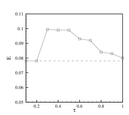
Figure 1: Kinetic energy of the SabraP model for $\nu=10^{-5}$ as a function of $\tau$. The constant reference line corresponds to the kinetic energy computed for the Sabra model without polymer.

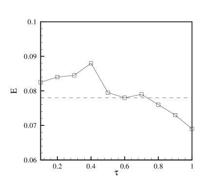
Figure 2: Kinetic energy of the SabraP model for $\nu=10^{-6}$ as a function of $\tau$. The constant reference line corresponds to the kinetic energy computed for the Sabra model without polymer.

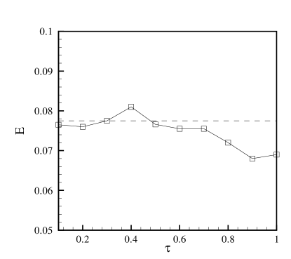
Figure 3: Kinetic energy of the SabraP model with polymer for $\nu=10^{-8}$ as a function of $\tau$. The constant reference line corresponds to the kinetic energy computed for the Sabra model without polymer.

By inspecting the three figures, one can safely state that the SabraP model shows drag reduction. In particular, for all cases, there is an optimal choice of $\tau$ for which the effect of drag reduction is maximal. For $\tau\to 0$ and $\tau\to\infty$ drag reduction decreases and eventually we enter a region of parameters where we observe drag enhancement. Moreover, for fixed value of $\tau$ and decreasing values of $\nu$, drag reduction decreases, reaching a mere few per cents for $\nu=10^{-8}$.

IV.2 Which scales are responsible for drag reduction?

To understand which scales are responsible for the drag reduction, we compare $\langle|u_{n}|^{2}\rangle$ for both models with $\nu=10^{-5}$, again at the same power input. This is shown in Fig. 4.

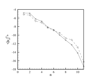
Figure 4: A comparison of the average energy shell-by-shell for the Sabra (dotted line with circles) and the SabraP (continuous line with squares) models. Drag reduction is seen is the relative increase in energy for small values of $n$ on the expense of large values of $n$.

This figure teaches us an interesting and important lesson. It is clear that the drag reduction is due to the relative increase in $\langle|u_{n}|^{2}\rangle$ for small values of $n$, and that this occurs on the expense of a relative decrease in $\langle|u_{n}|^{2}\rangle$ for high values of $n$. This finding is in close correspondence with similar conclusions obtained for the FENE-P model, both in homogeneous and channel flows 03ACLPP .

IV.3 The dissipative scale

In some theories of drag reduction it was proposed that the dissipative scale is increased in the viscoelastic flow, and that somehow this is responsible for the phenomenon 69Lum ; 90Gen ; 00SW . To test this possibility we plot in Fig. 5 the quantity $\langle k^{2}_{n}|u_{n}|^{2}\rangle$ as function of $n$.

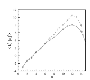
Figure 5: Energy dissipation computed for each shell for the Sabra model (dotted line with circles) and for the SabraP model (continuos line with squares)

This quantity peaks at the dissipative scale, i.e. the Kolmogorov scale. Inspecting figure (5) teaches us that the dissipative scale has not changed at all between the Sabra and the SabraP models, even though the latter certainly exhibits drag reduction. Thus, as indicated before, drag reduction should be understood as a phenomenon of the energy containing scales rather than the dissipative scales.

IV.4 Dynamical signature of drag reduction

The similarity between the FENE-P and its shell analog transcends statistical quantities. To observe the close dynamical similarity it is instructive to consider the quantity

$$\Pi=i\Sigma_{n}u^{*}_{n}\Phi_{n}(B,B)-i\Sigma_{n}u_{n}\Phi^{*}_{n}(B,B)\ ,$$ (18)

which describes the exchange between the kinetic energy $E_{u}$ and the “polymer” or “elastic” energy $E_{B}$.

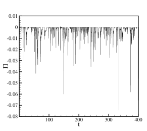
Figure 6: Time behavior of the quantity $\Pi$ as defined in the text

In figure (6) we show a time series of $\Pi$ for $\nu=10^{-5}$. $\Pi$ is always negative; the effect of the “polymers” is to drain energy form the kinetic energy. Moreover the dynamics of $\Pi$ is strongly intermittent which is a feature already observed in the DNS of the FENE-P model. The numerical simulations indicate the conclusion that the model introduced in this paper shows drag reduction in a way qualitatively close to the observed behaviour of the FENE-P model 02ACP .

We note in passing that it is not the first time that shell models seem to reproduce many of the features of turbulent flows; it is gratifying however that we can present a similar success even when we include relatively non trivial effects induced by polymer dynamics.

V Mechanism for drag reduction

This is the central section of this paper, in which we propose a detailed mechanism for drag reduction in the present model. We begin by analyzing the necessary conditions for drag reduction.

V.1 Necessary condition for drag reduction

To derive a necessary condition for drag reduction, let us consider the equation for the total energy, which reads:

$${\rm d}E/{\rm d}t=\Sigma_{n}\Big{[}\frac{1}{2}\left(f_{n}u_{n}^{*}+f_{n}^{*}u_{n}\right)-\nu k_{n}^{2}u_{n}u_{n}^{*}$$

$$-{1\over\tau}B_{n}B_{n}^{*}\Big{]}\ .$$ (19)

At steady state, with power input maintained constant at $P$, we have

$$P=\Sigma_{n}\left[\nu k_{n}^{2}u_{n}u_{n}^{*}+{1\over\tau}B_{n}B_{n}^{*}\right]$$ (20)

All the terms on the RHS are strictly positive. Since the energy input $P$ is constant for the Sabra and the SP models, we get

$$\Sigma_{n}k_{n}^{2}\left[(u_{n}u_{n}^{*})_{S}-(u_{n}u_{n}^{*})_{SP}\right]>0.$$ (21)

On the other hand if the SP model is to be drag reducing, we must have

$$\Sigma_{n}\left[(u_{n}u_{n}^{*})_{S}-(u_{n}u_{n}^{*})_{SP}\right]<0.$$ (22)

The only way (21) and (22) can hold simultaneously is if for small $k_{n}$, $|u_{n}|_{SP}>|u_{n}|_{S}$, and sufficiently larger to compensate for the fact that at large $k_{n}$, $|u_{n}|_{SP}<|u_{n}|_{S}$. This means that the kinetic energy plotted versus $k$ has to display an increased slope at least somewhere for drag reduction to take place. We have seen this already in Fig. 4. We show this important phenomenon once more in a log-log plot in Fig. 7, in which also the $B_{n}$-spectrum is shown for future reference.We see very clearly the crossing that occurs between the $u_{n}$ spectrum of the SabraP model and the Sabra counterpart, which is the necessary condition for drag reduction. Note that the increase in slope is a necessary but not a sufficient condition for drag reduction. We may increase the slope but not enough to cross the Sabra spectrum, or cross but not far enough to compensate for the reduced kinetic energy at large $k$.

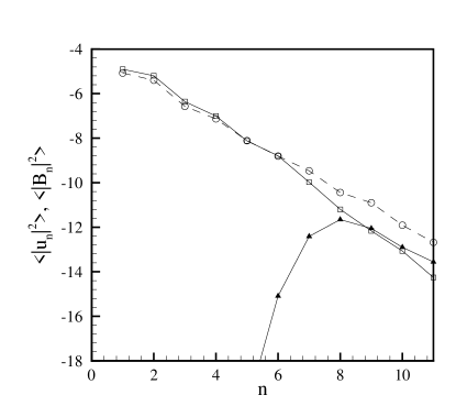
Figure 7: Energy spectrum of the SabraP model (continuos line with squares) and the Sabra model (continuos line with circles) for $\nu=10^{-6}$. The continuos line with black triangles represents the energy spectrum of the $B$ field.

V.2 Typical scales related to the polymer

A discussion of the mechanism of drag reduction calls for pointing out the existence of two typical scales that were already introduced in the past in the literature on drag reduction. The first is the Lumley scale, $k_{c}$, which is defined by the relaxation time of the polymer being of the same order as the eddy turn over time. For our model this scale satisfies

$$u(k_{c})k_{c}\sim\tau^{-1}\ .$$ (23)

Note that by definition this scale is Reynolds number independent.

The other scale, that we refer to as the de Gennes scale $k_{g}$, is where the kinetic energy on the scale $k_{g}$ is of the same order as the elastic energy:

$$u^{2}(k_{g})\sim B^{2}(k_{g})\ .$$ (24)

In fact, in the SabraP model the scales so defined appear to be very close, if not identical to each other. In particular, we will show presently that also $k_{g}$ is Reynolds number independent. To demonstrate the equivalence of the two scales we first exhibit in Fig. 8 the numerical estimate of $k_{c}$.

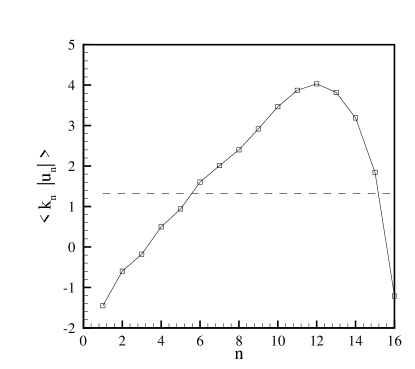
Figure 8: The inverse of the “eddy turn over time” $\sqrt{\langle E_{n}\rangle}k_{n}$ as a function of $k_{n}$ (continuous line with squares). The constant reference dotted line is $\tau^{-1}$. The crossing in inertial range identified $k_{c}$. In this figure $\nu=10^{-5}$, $\tau=0.4$.

The physical significance of $k_{c}$ is not in the accidental identity of two time scales, but rather that for $k$-vectors smaller than $k_{c}$ the effect of the $B_{n}$ field on the energy flux is negligible, but not so for $k$-vectors larger than $k_{c}$. To see this introduce two quantities related to the energy flux in the SabraP model, namely:

$$S_{n}=\left\langle Im(u_{n-1}^{*}u_{n}^{*}u_{n+1})\right\rangle$$ (25)

$$T_{n}=\left\langle Im(B_{n-1}^{*}u_{n}^{*}B_{n+1})\right\rangle$$ (26)

The physical meaning of the two quantities is rather clear: $S_{n}$ describes the flux of kinetic energy from large scale to small scales due to non linear terms, while $T_{n}$ describes the flux of kinetic energy to the polymer field. We expect that for $k_{n}$ near $k_{c}$, the effect of $T_{n}$ cannot be neglected in the dynamics, i.e. the average energy flux for the velocity field $G_{n}=S_{n}-T_{n}$ begins to change with respect to what it is observed in the Sabra model.

In figure (9) we show the quantity $G_{n}$ computed for the same model parameters of figure (8). The symbols refer to the Sabra model while the continuous line corresponds to the SabraP model. In the vicinity of $n_{c}\sim 5.5$ the two models show a different behaviour and in particular the SabraP model shows a decrease of the total energy flux $G_{n}$ as previously claimed.

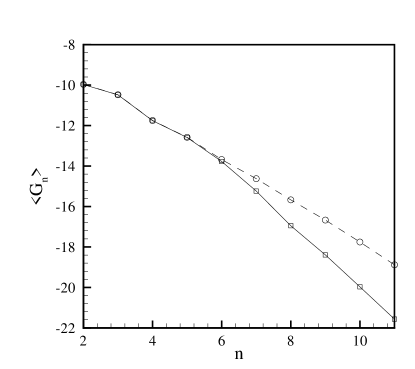
Figure 9: The average energy flux $G_{n}$ computed for the SabraP model (continuous line with squares) and the Sabra model (dotted lines with circles).

Regarding the scale $k_{g}$, it can be read from the spectrum shown in Fig. 7, in which $\nu=10^{-6}$. In Fig. 10 we show the analogous spectra for $\nu=10^{-8}$. Clearly $k_{g}$ did not change at all, in agreement with our assertion that it is Reynolds independent. Finally, we note that in all the figures shown $k_{c}$ and $k_{g}$ are of the same order of magnitude, and in the sequel we do not distinguish between the two.

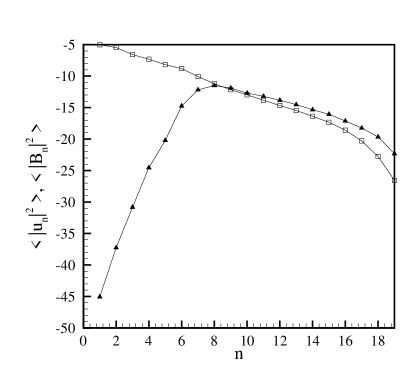
Figure 10: Energy spectrum of the SabraP model (continuous line with squares). The line with black triangles represents the energy spectrum of the $B$ field.

V.3 The effect of the polymer at large $k$-vectors

In this subsection and the next we discuss the effect of the $B_{n}$ field on the $u_{n}$ field for $k$-vectors much larger and much smaller than $k_{c}$. We will show that the spectrum $\langle|u_{n}|^{2}\rangle$ exhibits essentially the same scaling exponent as the Sabra model, but the amplitude is affected by the presence of the $B_{n}$ field. This will be an important ingredient in the mechanism of drag reduction.

Begin with $k_{n}$ large, $k_{n}\gg k_{c}$. In this regime the effect of the relaxation time $\tau$ on the dynamics of the $B_{n}$ field is completely negligible. The dynamics of $B_{n}$ is dominated by its coupling to $u_{n}$, simply because $u_{n}k_{n}\gg\tau^{-1}$. But then in this regime the dynamics is like the one of MHD which had been analyzed in detail in 03CCGP . The central conclusion of that analysis is that up to intermittency corrections, the spectra of both the $B_{n}$ and the $u_{n}$ fields exhibit a scaling exponent $\zeta_{2}=2/3$. Indeed, inspecting Fig. 10, we see that for large $k_{n}$ the two spectra have similar slopes, although intermittency affects the two spectra in a different way.

On the other hand, the amplitudes of the two spectra need not be the same. The relative displacement of the two power laws is determined by numerical details in the model. To estimate this displacement we will estimate the amplitudes of the two spectra at the dissipative scale. The contribution to the dissipation of $u$ is mainly from the small scales, i.e. very large values of $k_{n}$. We can define an effective scale $k_{d}$ the scale at which energy dissipation peaks:

$$\Sigma k_{n}^{2}\langle|u_{n}|^{2}\rangle\sim k_{d}^{2}\langle|u_{d}|^{2}\rangle$$ (27)

where $u_{d}=u(k_{d})$, and $k_{d}$ is of the order of the Kolmogorov scale. Since we found that the dissipative scale hardly changes when we add the coupling to the $B_{n}$ field, we can deduce from (20) that

$$\langle|u_{d}|^{2}\rangle_{SP}-\langle|u_{d}|^{2}\rangle_{S}\approx\sum_{n}\frac{\langle|B_{n}|^{2}\rangle}{\nu\tau}\ .$$ (28)

On the other hand, the sum on the RHS of Eq. (28) is a geometric sum dominated by the contribution of $B(k_{c})$ where $B_{n}$ is maximal. We thus estimate the relative displacement of the two spectra at high values of $k_{n}$ by

$$\langle|u_{d}|^{2}\rangle_{SP}-\langle|u_{d}|^{2}\rangle_{S}\approx\frac{\langle|B(k_{c})|^{2}\rangle}{\nu\tau}\ .$$ (29)

Thus to first approximation we expect the slopes of the two spectra to remain unchanged, maintained at a constant difference from each other as given by (29), until $k_{n}$ approaches $k_{c}$ from above, where the effect of the relaxation time $\tau$ on the dynamics of $B_{n}$ cannot be neglected.

V.4 The effect of the polymer at small $k$-vectors

Next we discuss the slope of the $u_{n}$ spectrum for $k_{n}\ll k_{c}$. This is very easy, since the amplitude of $B_{n}$ is very small due to the very efficient exponential damping by $\tau$. Thus the $u_{n}$ field hardly feels the coupling to $B_{n}$, and its slope, up to intermittency corrections, is again of the order of $\zeta_{2}=2/3$. Again, the amplitude is changed compared to the pure Sabra case, and this is the most important feature that is discussed next.

V.5 The tilt in the spectrum at $k_{n}\approx k_{c}$

Considering the spectrum in Fig. 10 we note that the $B_{n}$ spectrum increases rapidly when $k_{n}\to k_{c}$ from the left. To understand this phenomenon consider the equation of motion for $B_{n}$ at steady state. To leading order

$$0=\langle|{{\rm d}B_{n}\over{\rm d}t}|\rangle\sim\langle|c_{1}k_{n}u^{*}_{n+1}B_{n+2}|\rangle-{\langle|B_{n}|\rangle\over\tau}\ ,$$ (30)

where we have neglected terms of the order of $B_{n+1}$, but including them will lead to similar conclusions. Using the fact that $|k_{n+1}u^{*}_{n+1}\tau|\ll 1$, and since $|k_{n+1}u^{*}_{n+1}B_{n+2}|\leq|k_{n+1}u^{*}_{n+1}||B_{n+2}|$ we immediately conclude that

$$\langle|B_{n}|\rangle\ll\langle|B_{n+2}|\rangle\ .$$ (31)

We continue this argument recursively to estimate the largest polymer contribution $B(k_{c})$ as

$$\langle|B(k_{c})|\rangle\sim{\langle|B_{0}|\rangle\over\langle|k_{1}u_{1}|\rangle\langle|k_{3}u_{3}|\rangle...\langle|k_{c-1}u_{c-1}|\rangle\tau^{n_{c}/2}}$$ (32)

where $\lambda^{n_{c}}=k_{c}$.

In the vicinity of the scale $k_{c}$, we have to leading order in $B$ in the kinetic energy equation,

$$0 = -k_{n}S_{n+1}-bk_{n}S_{n}+(1+b)k_{n-2}S_{n-1}$$ (33)

$$- k_{n}\langle u_{n}^{*}B^{*}_{n+1}B_{n+2}\rangle\ .$$

When the amplitude of the polymer goes to zero ($B_{n}\to 0~{}\forall n$) the only solution is the well known scaling law $S_{n}\propto k_{n}^{-1}$. However the last term in (33) forces now a tilt in the spectrum. Its sign is exactly such that $S_{n-1}$ has to increase compared to $S_{n}$ and respectively $S_{n+1}$. Of course, for $k_{n}\ll k_{c}$ the effect of the $B_{n}$ field on the $u$-spectrum is again negligible, and therefore the spectral slope will settle back to the Sabra value. However if the tilt in the vicinity of $k_{c}$ results in crossing the Sabra spectrum we would have a whole spectral range where the energy is higher.

We therefore conclude that the existence of drag reduction depends rather heavily on the sign of the energy transfer at scales close to $k_{c}$. To check the sign directly in the numerics and thus to substantiate the existence of the tilt we return to the equations of motion and write

$$\!\!\!\frac{d}{dt}|u_{n}|^{2}\!\! = \!\!\Psi^{(n)}_{1}(u,u,u)-\Psi^{(n)}_{2}(u,B,B)-\nu k_{n}^{2}|u_{n}|^{2}\ ,$$

$$\!\!\!\frac{d}{dt}|B_{n}|^{2}\!\! = \!\!\Psi^{(n)}_{3}(u,B,B)+\Psi^{(n)}_{2}(u,B,B)\!-\!\frac{1}{\tau}|B_{n}|^{2}\ ,$$ (34)

where the term $\Psi_{1}^{(n)}(u,u,u)$ represents the kinetic energy flux of the field, while $\Psi^{(n)}_{2}(u,B,B)$ is the energy flux going from the velocity field to the polymer field. Finally, term $\Psi^{(n)}_{3}(u,B,B)$ is the flux of energy of the polymer field due to the transport of the velocity field. Figure (11) shows $\Psi^{(n)}_{1}$, $-\Psi^{(n)}_{2}$ and $\Psi^{(n)}_{3}$ for $\tau=0.4$ and $\nu=10^{6}$, the same parameters of figure (7). It is important to observe that $\Psi^{(n)}_{1}$ becomes positive for $n>n_{c}$. For a given $n$ the term $\Psi^{(n)}_{1}$ can be written as $\Psi^{(n)}_{1}=L_{n}-S_{n}$ where $L_{n}$ is the amount of energy flux given from the large scale to scale $k_{n}$ and $S_{n}$ is the amount of energy flux given from scale $k_{n}$ to smaller scales. It follows that when the energy flux is constant $L_{n}=S_{n}$ and therefore $\Psi^{(n)}_{1}(n)=0$. On the other hand, a positive value of $\Psi^{(n)}_{1}(n)$ implies that $L_{n}>S_{n}$. This is exactly what is shown in figure (11). The imbalance of the energy flux $\Psi^{(n)}_{1}$ is compensated by the flux of energy from $u_{n}$ to $B_{n}$, given by the term $-\Psi^{(n)}_{2}$. It is interesting to observe that the last term in the balance equation, namely $\Psi^{(n)}_{3}$, is rather small, i.e. the effect of an energy cascade of the polymer is rather weak.

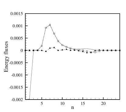
Figure 11: Energy fluxes for the SabraP model. The continuous line corresponds to the fluxes of the kinetic energy $\Psi^{(n)}_{1}$. The squares correspond to $-\Psi^{(n)}_{2}$. The dashed line with black triangles is $\Psi^{(n)}_{3}$

V.6 Discussion

While we have been able so far to describe a convincing scenario for drag reduction, we still should explain the mechanism for the increase of the large scale energy. Since the field $B_{n}$ is negligible for small $n$, the average energy flux per unit time at small $n$ must equal the input work per unit time at the largest scales. However, the energy flux does show time and scale fluctuations which could behave differently for the Sabra and SabraP models. More specifically let us consider the quantity $G_{n}$ defined in Subsect. V.2. As already discussed, $G_{n}$ represents the energy flux at scale $k_{n}$ due to both the non linear terms in the velocity field and the non linear term in the $B_{n}$ field. In terms of $G_{n}$, we can build a large scale energy flux $W_{L}=G_{2}+G_{3}+G_{4}$ which represents the full amount of energy flux across the largest scales, namely across $k$-vectors $k_{n}<k_{c}$, for which the average energy flux is invariant to changing Sabra to SabraP. The definition of $W_{L}$ is such that $W_{L}>0$ means an energy flux from large scales to small scales. In figure (12), we show the probability distribution of $W_{L}$ for both models, with numerical parameters $\nu=10^{-5}$ and $\tau=0.4$. The vertical line in the figure indicates the average value, which, as expected is invariant. As one can observe, the two probability distributions show a substantial difference for negative values of $W_{L}$: in the SabraP model one can have larger and more frequent negative values of the energy flux. This can happen even if the instantaneous value of the total energy per unit time obtained by the polymer field from the velocity field is always positive! Qualitatively this means that while the velocity field is always forcing the polymer field, at very large scales the flux can, from time to time, be reversed, and the polymer field forces there the velocity. This is how the amplitude of the energy spectrum is being increased on the average.

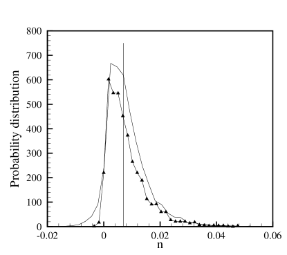
Figure 12: Probability distribution functions of $W_{L}$ for Sabra model (line with black triangles) and SabraP model (continuous line).

Clearly, this mechanism could not work unless the “forcing” by the polymer field acted in phase with the growing kinetic energy. In order to clarify this further we present two time-series of the kinetic energy and $W_{L}$, in Fig. (13) for the Sabra model, and in Fig. (14) for the SabraP model.

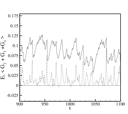
Figure 13: Time series of the kinetic energy (continuous line) and $2\times W_{L}$ (dotted line) for the Sabra model.

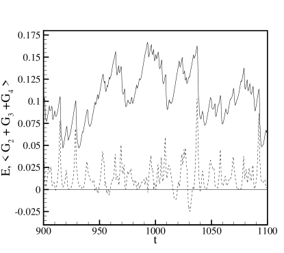
Figure 14: Time series of the kinetic energy (continuous line) and $2\times W_{L}$ (dotted line) for the SabraP model.

A close inspection of the figures shows that the reverse of the energy flux $W_{L}$ occurs exactly during the growing phase of the kinetic energy, leading therefore to a larger value of the instantaneous kinetic energy. This in phase mechanism is responsible for drag reduction. Note that this mechanism strongly depends on the large scale dynamics and the value of $k_{c}$. For $k_{n}$ larger than $k_{c}$ no significant difference in the statistical behaviour of the energy flux is observed. However, the amount of energy forcing, due to the polymer at large scale, can depend on the Reynolds number, at least in the SabraP model. If this is the case, then drag reduction should depend on the Reynolds number only through the two relevant scales appearing in the systems, namely $k_{c}$ and $\lambda_{T}$, the latter being the Taylor microscale

$$\lambda_{T}\equiv\sqrt{\frac{E_{u}}{\sum k_{n}^{2}|u_{n}|^{2}}}\ ,$$ (35)

which also depends on $\tau$ in the SabraP model. Because the drag is a dimensionless quantity, we argue that the only way in which the Reynolds number may appear in the drag reduction is by means of the dimensionless quantity $\mu=k_{c}\lambda_{T}(\tau)$.

There is a simple argument, proposed in the next section, which explains why at large Reynolds numbers one may observe the same qualitative mechanism, i.e. drag reduction, with smaller effects on the kinetic energy. As a matter of fact, the numerical results show that drag reduction reaches its maximum for $\mu\sim 1$

VI Predictions of the theoretical mechanism

We summarize the mechanism of drag reduction using the cartoon shown in Fig. 15.

Figure 15: Schematic of the effect of polymers in drag reduction on the turbulence energy spectrum. Dotted line: neat fluid. Solid line: polymeric solution. The spectral slope is unchanged for large and small scales, while at scale $k_{c}$ there is a significant upward tilt.

The tilt in the spectrum occurs in the vicinity of $k_{c}$, with the asymptotic slope for $k_{n}\ll k_{c}$ and $k_{n}\gg k_{c}$ remaining essentially unchanged. With such a spectrum the two inequalities (21) and (22) are obviously obeyed.

The difference in the spectra for $k_{n}\gg k_{c}$ is determined predominantly by Eq. (28). This equation predicts that this difference will be greatly increased when the Reynolds number is increased (i.e. when $\nu\to 0$), see Fig. 16. Of course, if this happens we can lose the whole effect of drag reduction, since the amount of tilt at $k_{c}$ is basically independent of $\nu$. We need to maintain the spectral difference small enough for the tilt to effect a crossing of the spectrum of SabraP and Sabra. Also the position of $k_{c}$ is important. If we reduce $k_{c}$ (i.e. increase $\tau$) the tilt is too far to the left and therefore it will fail to increase the energy. In fact it can be drag enhancing. The combined effect of decreasing $\nu$ and increasing $\tau$ is shown in Fig. 16.

Figure 16: Schematic of the turbulence energy spectrum when the polymer relaxation time scale is too slow, and the Reynolds number is too large.

Needless to say, also if we decrease $\tau$ too much we may lose drag reduction since the tilt will be pushed to the irrelevant dissipative range where no energy containing modes exist. Also, if $\tau$ becomes too low, $B_{n}$ becomes smaller, and the amount of tilt is decreased, as can be seen directly from Eq. (33). Although decreasing the field $B_{n}$ brings the spectra closer together in the large $k_{n}$ regime, the tilt may not suffice to reduce the drag. Such a situation is shown schematically in Fig. 17.

Figure 17: The relaxation time $\tau$ is to low.

Actually, using the language introduced in the previous section and the above discussions, we are able to give another argument to understand how drag reduction could depend on the Reynolds number. As previously said, the relevant dimensionless number in the system is $\mu=k_{c}\lambda_{T}$. If $\tau\rightarrow\infty$ then $k_{c}\rightarrow 0$ and we know that drag reduction must be inhibited. It follows that for $\mu\rightarrow 0$ we cannot observe drag reduction. For fixed $k_{c}$ and increasing Reynolds, $\lambda_{T}(\tau)$ decreases as well, although not necessarily as $Re^{-1/2}$, where $Re$ is the Reynolds number. Then, for fixed $\tau$ and increasing Reynolds number we should observe a decreasing effect of drag reduction, as observed in our numerical simulation. The same reasoning can be applied to get information for small Reynolds numbers, as the following argument shows. For $\tau\rightarrow 0$ we have already shown that no drag reduction is possible simply because $k_{c}\rightarrow\infty$. This is equivalent to say that when $\mu$ becomes too large there cannot be any drag reduction. It follows that for small $Re$, i.e. for large $\lambda_{T}$, drag reduction disappears.

VII Conclusions and Discussions

In this paper we discussed several points concerning the possible formulation of a theory for drag reduction in turbulent flow with dilute polymer. It is worthwhile, therefore, to review the main points.

A) We have introduced a shell model resembling the dynamical properties of the FENE-P equations. Beside any theoretical considerations, the model shows drag reduction in a way close to what already observed in the numerical simulations of the FENE-P model. The implications of this result is that one need not focus on boundary effects or dynamical properties of coherent structure in order to capture the basic physics of drag reduction.

B) There exist a relevant scale in the system, $k_{c}$ defined by the so called ’time criterion’, i.e. $u(k_{c})k_{c}\sim\tau^{-1}$. In the vicinity of this scale there is a tilt in the spectrum which causes a crossing of the SabraP velocity spectrum above the Sabra spectrum for $k_{n}<k_{c}$. This in its turn means an increase in the kinetic energy at large scales. Drag reduction can be physically understood in terms of the energy exchanges between the velocity field and the polymer field for $k_{n}\sim k_{c}$. We have succeeded in proposing a coherent picture, based on the equation of motions, for the dynamics which is in close agreement with the numerical results.

C) Drag reduction is a property of large scale flow and its dynamics. This implies that a quantitative description of drag reduction must depend on the details of the flow, the forcing mechanism as well as the Reynolds numbers. Although a general qualitative mechanism should occur in all drag reduction flow, the amount of the drag reduction itself depends on how much energy is intermittently given to large scale velocity. Thus large scale fluctuations are important for a quantitative theory.

D) Drag reduction by no means could be reduced to the dynamics at the dissipation scale. Although drag reduction could be Reynolds dependent, drag reduction cannot be reduced to a simple increase of the dissipation length. Actually, the dissipation scale does not seem to be affected by drag reduction.

- (1) J.L. Lumley, Ann.Rev. Fluid Mech. 1, 367 (1969).
- (2) P.S. Virk, AIChE J. 21, 625 (1975).
- (3) T.S. Luchik and W.G Tiederman, J.Fluid Mech 190 241, (1987).
- (4) J.M.J. de Toonder, M.A. Hulsen, G.D.C. Kuiken and F.T.M Niewstadt, J. Fluid Mech., 337, 193 (1997).
- (5) R.B. Bird, C.F. Curtiss, R.C. Armstrong and O. Hassager, Dynamics of Polymeric Fluids Vol.2 (Wiley, NY 1987)
- (6) A.N. Beris and B.J. Edwards, Thermodynamics of Flowing Systems with Internal Microstructure (Oxford University Press, NY 1994).
- (7) E. de Angelis, C. Casciola, R. Benzi, and R. Piva, Phys. of Fluids, submitted.
- (8) C.D. Dimitropoulos, R. Sureshdumar and A.N. Beris, J. Non-Newtonian Fluid Mech. 79, 433 (1998).
- (9) E. de Angelis, C.M. Casciola and R. Piva, Computers and Fluids, 31, 495 (2002).
- (10) E. Balkovsky, A. Fouxon V. Lebedev Phys. Rev. E, 64, 056301 (2001).
- (11) P.-G. de Gennes, Introduction to Polymer Dynamics, (Cambridge, 1990)
- (12) R. Benzi and I. Procaccia, ”A simple model for drag reduction”, Phys. Rev. Lett., submitted. Also:cond-mat/0210523
- (13) P. Giuliani and V. Carbone, Europhys. Lett. 43, 527 (1998).
- (14) E.S.C. Ching, Y. Cohen, T. Gilbert and I. Procaccia, Phys. Rev. E 67, 016304 (2003)
- (15) V.S. L’vov, E. Podivilov, A. Pomyalov, I. Procaccia and D. Vandembroucq., Phys. Rev. E 58 1811 (1998).
- (16) E. de Angelis, C. Casciola, V.S. L’vov, R. Piva and I. Procaccia, Phys. Rev. E, submitted.
- (17) K. R. Sreeinvasan and C. M. White, J. Fluid Mech. 409, 149 (2000).