Spiral and Taylor vortex fronts and pulses in axial through-flow

Abstract

The influence of an axial through-flow on the spatiotemporal growth behavior of different vortex structures in the Taylor-Couette system with radius ratio $\eta=0.5$ is determined. The Navier Stokes equations (NSE) linearized around the basic Couette-Poiseuille flow are solved numerically with a shooting method in a wide range of through-flow strengths $Re$ and different rates of co- and counterrotating cylinders for toroidally closed vortices with azimuthal wave number $m=0$ and for spiral vortex flow with $m=\pm 1$. For each of these three different vortex varieties we have investigated (i) axially extended vortex structures, (ii) axially localized vortex pulses, and (iii) vortex fronts. The complex dispersion relations of the linearized NSE for vortex modes with the three different $m$ are evaluated for real axial wave numbers for (i) and over the plane of complex axial wave numbers for (ii, iii). We have also determined the Ginzburg-Landau amplitude equation (GLE) approximation in order to analyze its predictions for the vortex stuctures (ii, iii). Critical bifurcation thresholds for extended vortex structures are evaluated. The boundaries between absolute and convective instability of the basic state for vortex pulses are determined with a saddle-point analysis of the dispersion relations. Fit parameters for power-law expansions of the boundaries up to $Re^{4}$ are listed in two tables. Finally, the linearly selected front behavior of growing vortex structures is investigated using saddle-point analyses of the dispersion relations of NSE and GLE. For the two front intensity profiles (increasing in positive or negative axial direction) we have determined front velocities, axial growth rates, and the wave numbers and frequencies of the unfolding vortex patterns with azimuthal wave numbers $m=0,\pm 1$, respectively.

I INTRODUCTION

The Taylor-Couette system review of fluid flow in the annulus between concentric cylinders with the inner and the outer one rotating with different velocities is one of the simplest examples of a driven nonlinear dissipative system that shows spontaneous pattern formation out of an unstructured basic state that is stable at small driving CRO-HOH . This basic flow state is stationary and axially and azimuthally homogeneous and shows only a radial variation across the annular gap. It consists of a superposition of circular Couette flow (CCF) in azimuthal direction and of an annular Poiseuille flow (APF) in axial direction if as in our case an axial through-flow is imposed. Axially periodic vortex flow solutions bifurcate CHO-IOO ; GOL-STE-SCH-LAN out of this homogeneous basic flow when the rotation rate of the inner cylinder is sufficiently high. These primary bifurcation thresholds to periodic vortex stuctures have been the aim of many linear stability analyses of the basic flow state DIP-PRI ; TAK-JAN ; NG-TUR ; LAN-TAG-KOS-SWI-GOL ; GEB-GRO ; MES-MAR .

For the radius ratio $\eta=0.5$ and the parameter ranges of rotation rates and through-flow investigated here in this work three spatiotemporally differing primary vortex structures are relevant: Rotationally symmetric, toroidally closed vortices with azimuthal wave number $m=0$ that move in downstream direction with the APF — for shortness we call this flow state Taylor vortex flow (TVF) although the presence of an axial through-flow modifies the genuine stationary TVF stucture. And, furthermore, spiral vortex flow (SPI) consisting of either left spiral vortices (L-SPI) with $m=1$ or right spiral vortices (R-SPI) with $m=-1$.

L-SPI and R-SPI are axial mirror images of each other in the absence of axial through-flow with the latter breaking the mirror symmetry of the former. While rotating azimuthally into the same direction as the inner cylinder L-SPI propagate axially opposite to R-SPI. This spiral dynamics is largely induced by the advective properties of the basic flow state. Furthermore, without through-flow the symmetry degenerate bifurcation treshold for these two symmetry degenerate SPI solutions is simultaneously also the bifurcation threshold for a vortex flow solution called ribbons CHO-IOO . This solution consists right at threshold of a linear superposition of L-SPI and R-SPI with equal amplitude and it becomes further away from threshold a genuine nonlinear vortex flow solution. However, here we are dealing only with linear vortex flow fields that may be superimposed with arbitrary amplitudes as well as wave numbers and that are evolving separately from each other according to the linear field equations. Thus we do not need to discuss ribbons separately from our general investigation of linear vortex modes with general axial and azimuthal wave numbers.

In this work we quantitatively determine the influence of an axial through-flow on the spatiotemporal growth properties of linear perturbations of the basic flow state with azimuthal wave numbers $m=0$ and $m=\pm 1$, i.e., of toroidally closed vortices and of spiral vortices, repectively. In each case we investigate (i) axially extended structures, (ii) pulses of axially localized wave packets of vortices, and (iii) vortex fronts.

In Sec. II we describe the system, we briefly review the linearized Navier-Stokes equations (NSE) for the eigenvalue problem describing vortex perturbations, and we give details of our numerical procedure to solve the eigenvalue problem. In Sec. III we discuss the spatiotemporal structure, symmetry properties, and bifurcation thresholds for onset of axially extended vortex perturbations of the form $e^{i(kz+m\varphi)}$ with real axial wave number $k$ and different azimuthal wave numbers $m$ in the absence and presence of an axial through-flow. In Sec. IV we consider axially localized wave packets consisting of superpositions of vortex eigenmodes of the linear NSE. Here we determine among others the boundary between convective and absolute instability of the basic flow against growth of vortices with a particular $m$ by a saddle point analysis of the linear complex dispersion relation of the NSE over the plane of complex axial wave numbers. In addition we also determine the Ginzburg-Landau amplitude equation (GLE) approximation for the dispersion relation for the sake of comparison. In Sec. V we evaluate the spatiotemporal properties of linearly selected vortex fronts using a saddlepoint analysis of the dispersion relation. Also here we compare with GLE results. The final section contains a summary.

II System

Here we describe the system and we provide definitions and equations. Then we briefly review the linearized equations for the eigenvalue problem describing vortex perturbations of the basic flow state. Finally we give details of our numerical procedure to solve the eigenvalue problem.

II.1 Setup

We consider the flow of an incompressible fluid in the annulus between two concentric cylinders of inner radius $r_{1}$ and outer radius $r_{2}$ with a gap width $d=r_{2}-r_{1}$. The boundary conditions at $r_{1}$ and $r_{2}$ are no-slip. The angular velocity of the inner and outer cylinder is $\Omega_{1}$ and $\Omega_{2}$, respectively. The associated Reynolds numbers are

$$R_{1}=\frac{d}{\nu}r_{1}\Omega_{1},\quad R_{2}=\frac{d}{\nu}r_{2}\Omega_{2},$$ (1)

where $\nu$ is the kinematic viscosity. An externally imposed axial through-flow is measured by the axial Reynolds number

$$Re=\frac{d}{\nu}\langle w\rangle$$ (2)

where the mean axial velocity $\langle w\rangle$ averaged over the annular cross section describes the total through-flow. We use also the relative control parameters

$$\mu=\frac{R_{1}}{R_{1c}(Re)}-1,\quad\epsilon=\frac{R_{1}}{R_{1c}(Re=0)}-1,$$ (3)

measuring the relative distance of the inner Reynolds number $R_{1}$ from the critical onset $R_{1c}$ of axially extended spiral vortices or Taylor vortices in the presence and in the absence $(Re=0)$ of through-flow, respectively epsT . In this notation

$$\mu_{c}=0\quad\mbox{and}\quad\epsilon_{c}(Re)=\frac{R_{1c}(Re)}{R_{1c}(Re=0)}-1$$ (4)

is the critical threshold for onset of the vortex flow in question. The relation between $\mu$ and $\epsilon$ is

$$\mu=\frac{\epsilon-\epsilon_{c}(Re)}{1+\epsilon_{c}(Re)}.$$ (5)

With infinitely long cylinders the only relevant parameter characterizing the geometry is the radius ratio $\eta=r_{1}/r_{2}$.

The velocity field $\bf u$ of the fluid is described by the Navier-Stokes equations (NSE) for incompressible fluid flow

$$\partial_{t}{\mathbf{u}}=\mbox{\bf\boldmath$\nabla$}^{2}{\bf u}-R_{1}({\bf u}\cdot\mbox{\bf\boldmath$\nabla$}){\bf u}-\mbox{\bf\boldmath$\nabla$}p,\quad\mbox{\bf\boldmath$\nabla$}\cdot{\bf u}=0.$$ (6)

Here and in the following we scale positions by the gap width $d$, the velocity ${\bf u}$ by the velocity $r_{1}\Omega_{1}$ of the inner cylinder, time $t$ by the momentum diffusion time $d^{2}/\nu$ across the gap, and the pressure $p$ by $\rho r_{1}\Omega_{1}\nu/d$ with $\rho$ denoting the constant mass density of the fluid. Furthermore we decompose the velocity field

$${\bf u}=u{\bf e}_{r}+v{\bf e}_{\varphi}+w{\bf e}_{z}$$ (7)

into radial ($u$), azimuthal ($v$), and axial ($w$) components using cylindrical coordinates $r,\varphi,z$.

II.2 Basic flow state

The basic flow state ${\bf u}_{0}$ that is realized in the absolutely stable regime of inner Reynolds numbers $R_{1}$ below the thresholds for onset of Taylor and spiral vortex flow is rotationally symmetric, axially homogeneous, and constant in time. It consists of a linear superposition of circular Couette flow (CCF) in azimuthal direction, ${\bf e}_{\varphi}$, and of annular Poiseuille flow (APF) in axial direction, ${\bf e}_{z}$,

$${\bf u}_{0}=v_{CCF}(r){\bf e}_{\varphi}+w_{APF}(r){\bf e}_{z}$$ (8)

without any radial component. Here

$$v_{CCF}(r)=Ar+B/r,$$ (9)

and

$$w_{APF}(r)=Re\frac{r^{2}+Cln(r)+D}{E},$$ (10)

with

$$A = -\frac{\eta^{2}-\Omega_{2}/\Omega_{1}}{\eta(1+\eta)},$$ (11)

$$B = \frac{\eta(1-\Omega_{2}/\Omega_{1})}{(1-\eta)(1-\eta^{2})},$$ (12)

$$C = \frac{1+\eta}{(1-\eta)ln(\eta)},$$ (13)

$$D = \frac{(1+\eta)\ln(1-\eta)}{(1-\eta)\ln(\eta)}-\frac{1}{(1-\eta)^{2}},$$ (14)

$$E = -\frac{1}{2}R_{1}\frac{1-\eta^{2}+(1+\eta^{2})\ln(\eta)}{(1-\eta)^{2}\ln(\eta)}.$$ (15)

II.3 Linear eigenvalue problem of vortex perturbations

Let $\psi=(u,v,w,p)$ abbreviate the deviation fields from the basic flow state (8). Then the general solution of the NSE linearized in the deviation fields can be written as a superposition of modes of the form

$$\psi(r,\varphi,z,t)=\phi(r)e^{i(kz+m\varphi)}e^{\sigma t}$$ (16)

with axial wave number $k=2\pi/\lambda$ and integer azimuthal wave number $m$. The complex amplitude functions

$$\phi(r)=\left[U(r),V(r),W(r),P(r)\right]$$ (17)

depend on the mode indices $k,m$ and the radial coordinate $r$. The characteristic exponent $\sigma(k,m)$ is in general complex. It is decomposed here as follows

$$\sigma=\Re\sigma+i\,\Im\sigma=\gamma-i\omega$$ (18)

into the growth rate $\gamma$ and the characteristic frequency $\omega$ of the $k-m$ mode. Substituting the above solution ansatz into the linearized NSE yields

$$\sigma U=\left(\partial_{r}^{2}+\frac{1}{r}\partial_{r}-\frac{1+m^{2}}{r^{2}}-k^{2}\right)U+2FV$$

$$\qquad-\partial_{r}P-im\left(\frac{2}{r^{2}}V+FU\right)-ikHU$$ (19)

$$\sigma V=\left(\partial_{r}^{2}+\frac{1}{r}\partial_{r}-\frac{1+m^{2}}{r^{2}}-k^{2}\right)V+2GU$$

$$\qquad-\frac{im}{r}P+im\left(\frac{2}{r^{2}}U-FV\right)-ikHV$$ (20)

$$\sigma W=\left(\partial_{r}^{2}+\frac{1}{r}\partial_{r}-\frac{m^{2}}{r^{2}}-k^{2}\right)W-ikP$$

$$\qquad-imFW-IU-ikHW$$ (21)

$$\quad 0=\partial_{r}U+\frac{1}{r}U+\frac{im}{r}V+ikW.$$ (22)

The solution of this eigenvalue problem yields the characteristic exponent $\sigma$ and the associated eigenfunctions $\phi(r)$ as functions of $k,m$. Here

$$F(r) = \frac{R_{1}}{r}v_{CCF}(r)\quad,\quad G=-R_{1}A,$$ (23)

$$H(r) = R_{1}w_{APF}(r)\quad,\quad I(r)=\partial_{r}H(r)$$ (24)

are quantities defining the basic flow state (8). The latter enters via the linearized advective term of the NSE.

In order to rewrite (II.3 - 22) into a system of first-order differential equations – which is advantageous for numerical reasons – we introduce three additional complex amplitude functions LAN-TAG-KOS-SWI-GOL

$$X = \partial_{r}U+\frac{1}{r}U-P\,,$$ (25)

$$Y = \partial_{r}V+\frac{1}{r}V\,,$$ (26)

$$Z = \partial_{r}W\,.$$ (27)

Using (25) and the continuity equation (22) one can then eliminate the pressure in Eq.(II.3) by $P=-X-ikW-\frac{im}{r}V.$ All in all one obtains in this way a system of 6 coupled, first-order differential equations

$$\partial_{r}{\bf X}={\cal L}\ {\bf X},$$ (28)

for the six variables

$${\mathbf{X}}=\left(U,V,W,X,Y,Z\right)^{T}$$ (29)

with

$${\cal L}=\left(\begin{array}[]{cccccc}-\frac{1}{r}&-i\frac{m}{r}&-ik&0&0&0\\ 0&-\frac{1}{r}&0&0&1&0\\ 0&0&0&0&0&1\\ L&2(i\frac{m}{r^{2}}-F)&0&0&0&0\\ -2(i\frac{m}{r^{2}}+G)&L+\frac{m^{2}}{r^{2}}&\frac{mk}{r}&-i\frac{m}{r}&0&0\\ I&\frac{mk}{r}&L+k^{2}&-ik&0&-\frac{1}{r}\\ \end{array}\right)$$ (30)

where

$$L=\sigma+\frac{m^{2}}{r^{2}}+k^{2}+imF+ikH.$$ (31)

II.4 Numerical procedures

We have solved the eigenvalue equations (28) numerically with a standard shooting method subject to the six boundary conditions,

$$U=V=W=0\quad\textrm{at}\quad r_{1}=\eta/(1-\eta)\,\,\textrm{and}\,\,r_{2}=1/(1-\eta)\,,$$ (32)

which make the eigenvalue spectrum discrete. To integrate from $r_{1}$ to $r_{2}$ we used a fourth-order Runge-Kutta formula STO-BUR with two step widths ( $\Delta r=1/200$ and 1/400, respectively) for a Richardson extrapolation. A Newton-Raphson method PRE-TEU-VET-FLA was then used to find the roots of the complex determinant of the $3\times 3$ matrix which ensures the vanishing of $U,V,W$ at the outer cylinder. We therefore vary in the Newton-Raphson procedure only two of the parameters ($\sigma,\eta,R_{1},R_{2},Re,m,k$) DIP-PRI that enter into (28) while keeping the others fixed. In this way we determine on the one hand the marginal threshold values of $R_{1}$ and $\omega$ with $\gamma=0$ for which the basic state is marginally stable against the growth of an extended perturbation with given $m$ and real axial wave number $k$ at specified parameters $\eta,R_{2},Re$. On the other hand we calculate for given $m,\eta,R_{1},R_{2},Re$ the complex eigenvalue $\sigma$ over the complex wave number plane – including as special case also the real $k$-axis. In each case we are interested only in the vortex modes with the largest growth rates for which the associated amplitude functions $\phi(r)$ display the least radial variation with the fewest number of nodes.

We present here results for the radius ratio $\eta=0.5$ in a range of outer Reynolds numbers $-150\leq R_{2}\leq 50$. In this parameter regime the vortex perturbations with the largest growth rates have in the absence of through-flow azimuthal wave numbers of either $m=0$ or $m=\pm 1$ LAN-TAG-KOS-SWI-GOL . We investigate here linear properties of such vortices with $m=0$ and $m=\pm 1$ in a through-flow of Reynolds numbers $0\leq Re\leq 20$.

III Axially extended vortex structures

Here we discuss the spatiotemporal structure, symmetry properties, and bifurcation thresholds for onset of axially extended vortex perturbations with real axial wave number $k$ and different azimuthal wave numbers $m$ in the absence and presence of an axial through-flow.

III.1 Spatiotemporal structure

Structure and dynamics of the vortex modes (16) are dominated by the fact that their phases are constant on any cylindrical surface, $r=const$, along lines given by the equation

$$z_{0}=-\frac{m}{k}\varphi+\frac{\omega(k,m)}{k}t\,.$$ (33)

Here the constant phase coming from the amplitude $\phi(r)$ is suppressed. Thus, on the $\varphi-z$ plane of such an ’unrolled’ cylindrical surface these lines of constant phase are straight.

III.1.1 Taylor vortex like patterns — $m$=0

For rotationally symmetric Taylor vortex like perturbations the line pattern of constant phases, $kz_{0}=n2\pi$, is parallel to ${\bf e}_{\varphi}$. The $m$=0 pattern is stationary for $Re=0$. Only for finite through-flow it propagates axially with phase velocity

$$w_{phase}=\frac{\omega}{k}$$ (34)

that is proportional to $Re$. The main reason for this is that the azimuthal flow of the basic CCF state is precisely parallel to the vortex lines of constant phase while the APF flow being perpendicular to them can advect them. The latter happens in our axially periodic system that does not exert any phase pinning at the axial boundaries as soon as $Re>0$.

III.1.2 Spiral patterns — $m\neq 0$

The vortex modes (16) with axial wave number $m\neq 0$ have spiral structure. When $m/k$ is positive (negative) the lines of constant phase $z_{0}(\varphi,t)$ (33) wind in a left spiral L-SPI (right spiral R-SPI) around the cylindrical surface $r=const$ with negative (positive) slope $\partial_{\varphi}z_{0}=-m/k$. The lines of constant phase and with it the whole spiral stucture rotates in $\varphi$ rigidly with angular velocity

$$\dot{\varphi}_{SPI}=\frac{\omega}{m}\,.$$ (35)

In the absence of an externally imposed through-flow, $Re$=0, this rotation proceeds for L-SPI and R-SPI alike into the same direction as the rotation of the inner cylinder. The reason is that the spiral perturbations are advected by the inner part of the azimuthal CCF which is relevant for the centrifugal instability leading to vortex generation. A model explaining this effect is presented in HOF-LUE .

There are two immediate consequences of this advective origin of the spiral dynamics induced by the inner cylinder’s rotation: (i) With the latter being by definition positive – in this work the inner cylinder is taken to rotate in positive $\varphi$-direction – also $\omega(k,m)/m$ is positive for $Re$=0. Hence, say, an $m=1$ ($m=-1$) spiral has positive (negative) frequency for $Re$=0. (ii) Then a L-SPI (R-SPI) being defined by $m/k>0$ ($m/k<0$) propagates for $Re$=0 upwards (downwards) with positive (negative) axial phase velocity

$$w_{phase}=\frac{\omega}{k}=\frac{m}{k}\dot{\varphi}_{SPI}$$ (36)

that is directly related to its positive angular velocity $\dot{\varphi}_{SPI}$.

An externally applied axial through-flow changes the axial phase velocities and frequencies of the $m=0$ and $m\neq 0$ vortex modes roughly proportional to $Re$, i.e.,

$$w_{phase}(k,m,Re)-w_{phase}(k,m,Re=0)\propto Re\,.$$ (37)

Simultaneously the rotation rates, $\dot{\varphi}_{SPI}=w_{phase}k/m$, of the spirals are changed accordingly. Thus, in each case the vortex frequencies are largely determined by the basic state’s advective properties, i.e., by the combination of azimuthal advection by $v_{CCF}$ and axial advection by $w_{APF}$.

III.2 Symmetries

Here we consider symmetry properties of axially extended vortex perturbations of the form (16) with real wave number $k$. Symmetry relations between different vortex fronts with complex wave number $Q$ are discussed later on in Sec. V.2.2.

Table 1 shows the symmetry transformations that leave the eigenvalue problem unchanged. They reflect (i) that ${\cal L}$ transforms under complex conjugation (indicated by an overline) as

$$\overline{{\cal L}(k,m,\sigma)}={\cal L}(-k,-m,\overline{\sigma})$$ (38)

and (ii) that the NSE (6) are invariant under an axial reflection $(z,Re,w)\longrightarrow(-z,-Re,-w)$.

Thus one infers, for example, that the growth rate (frequency) of the characteristic exponent $\sigma=\gamma-i\omega$ for $m=0$ vortices is an even (odd) function of $k$ and $Re$. For perturbations with $m\neq 0$ one finds that

$$\gamma(k,m,Re)=\gamma(-k,-m,Re) = \gamma(-k,m,-Re)=\gamma(k,-m,-Re)$$ (39)

$$\omega(k,m,Re)=-\omega(-k,-m,Re) = \omega(-k,m,-Re)=-\omega(k,-m,-Re)$$ (40)

and that the spatiotemporal structure including the amplitude functions of a L-spiral perturbation ($k/m>0$) at $Re>0$ is the same as that of a R-spiral ($k/m<0$) at $Re<0$. Note, however, that any finite through-flow breaks the axial mirror symmetry between L- and R-spirals at $Re=0$ so that, among others,

$$\gamma_{R}(-Re)=\gamma_{L}(Re)\neq\gamma_{R}(Re)=\gamma_{L}(-Re)$$ (41)

when $Re\neq 0$. But the symmetry relations are such that it suffices to investigate, say, positive $k$ combined together with either (i) $m>0$ only for positive and negative $Re$ or, equivalently, (ii) $m$ positive and negative for $Re>0$ only in order to get the complete linear information on both spiral vortex types.

III.3 Bifurcation thresholds

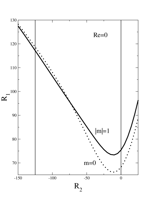
Figure 1: Critical bifurcation thresholds $R_{1c}(R_{2})$ for $m=0$ and $m=\pm 1$ vortex patterns with the respective critical wave numbers, $k_{c}(m,R_{2})$, as functions of $R_{2}$ in the absence of axial through-flow. The vertical lines mark the two representative outer Reynolds numbers $R_{2}=0$ and $R_{2}=-125$ that are investigated in more detail in this work. The radius ratio is $\eta=0.5$.

Figure 1 shows the critical bifurcation thresholds $R_{1c}(R_{2})$ for $m=0$ and $m=\pm 1$ vortex patterns with the respective critical wave numbers, $k_{c}(R_{2})$, as functions of $R_{2}$ in the absence of through-flow.

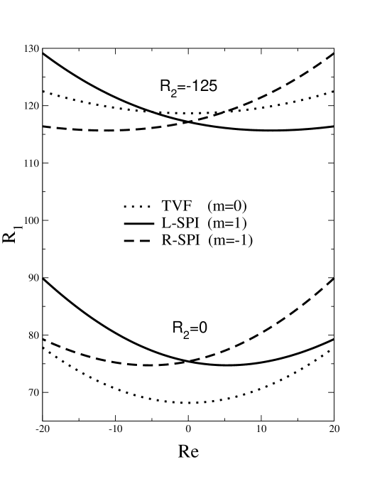
Figure 2: Evolution of the critical bifurcation thresholds $R_{1c}(Re)$ for $m=0$ and $m=\pm 1$ vortex patterns with through-flow Reynolds number $Re$. The two outer Reynolds numbers $R_{2}=0$ and $R_{2}=-125$ are marked in Fig. 1. The radius ratio is $\eta=0.5$.

The vertical lines in Fig. 1 mark the two outer Reynolds numbers $R_{2}=0$ and $R_{2}=-125$ for which we show in Fig. 2 as representative examples how the critical thresholds evolve with through-flow Reynolds number $Re$. The above discussed symmetry relation $\gamma_{R}(-Re)=\gamma_{L}(Re)$ between the growth rates of R- and L-spirals implies the corresponding relation between the respective bifurcation thresholds (full and dashed lines in Fig. 2). In the remainder of this paper we therefore restrict ourselves without loss of information to positive $Re$.

For small $Re>0$ the axial flow stabilizes the basic state against growth of TVF ($m=0$) and R-SPI ($m=-1$) perturbations. On the other hand, the bifurcation threshold for L-SPI ($m=1$) vortex patterns that propagate into the same direction as the through-flow decreases at small $Re$ and increases only at larger $Re$. The upwards shift of the $m=0$ threshold with increasing $Re$ is stronger than the one for $m=1$. Thus, eventually the latter comes to lie below the former and consequently the growth of L-spirals propagating into the same direction as the through-flow is favored for sufficiently large $Re$ even when $R_{2}=0$.

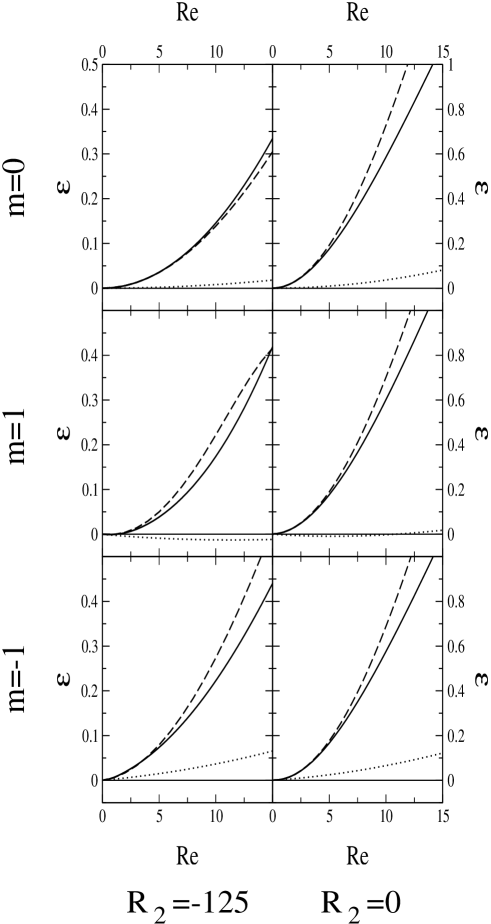
Figure 3: Stability boundaries of the basic flow state as functions of the through-flow Reynolds number $Re$. Dotted lines show the reduced critical bifurcation thresholds $\epsilon_{c}$ (4) for axially extended vortex patterns. The full (dashed) boundary lines, $\epsilon_{c-a}$, between the convectively and absolutely unstable parameter regions for vortex growth were obtained from the eigenvalues of the full NSE (the GLE approximation) – cf. Sec. IV. The radius ratio is $\eta=0.5$.

Dotted lines in Fig. 3 show the reduced critical threshold curves $\epsilon_{c}(Re)$ (4) as functions of $Re$ for the two representative outer Reynolds numbers $R_{2}=0$ and $R_{2}=-125$. The other lines in Fig. 3 are discussed in Sec. IV. Our numerical results for $\epsilon_{c}(Re)$ that were obtained in steps of $\delta Re=1$ were fitted in the range $Re=-20\cdots 20$ to the following expression

$$f=a_{1}Re+a_{2}Re^{2}+a_{3}Re^{3}+a_{4}Re^{4}\,.$$ (42)

The fit parameters $a_{n}$ are listed for different $R_{2}$ in Tables 2 and 3 for TVF ($m=0$) and L-SPI $(m=1)$, respectively. The threshold curves for R-SPI $(m=-1)$ are obtained according to Sec. III.2 from those for L-SPI by $Re\rightarrow-Re$, i.e., by changing the sign of the odd coefficients in Table 3.

IV Localized vortex perturbations

So far we have considered axially extended vortex perturbations of the form $\psi(r,\varphi,z,t)=\phi(r)e^{i(kz+m\varphi)}$ which are single eigenmodes of the operator ${\cal L}$ (30). For supercritical control parameters, $R_{1}>R_{1c}(m)$, a finite band of axial wave numbers can grow and with it also axially localized wave packets consisting of superpositions of vortex modes.

IV.1 Vortex packets

Let us consider first an infinitesimal initial perturbation with azimuthal wave number $m$ that is axially localized, i.e., a wave packet that consists of a superposition of vortex modes of different $k$ but common $m$ – an initial perturbation containing different $m$-modes would be just a sum of the above described vortex packets that would evolve independently of each other as long as the linear description is valid.

After fast transients have decayed a pulse like perturbation survives with axial wave numbers within the unstable band centered around the wave number of maximal growth $k_{max}(m)\simeq k_{c}(m)$. Since the above described wave packet contains vortex modes that can grow the pulse will grow as well. Simultaneously the pulse center travels axially for small $\epsilon$ with the critical goup velocity

$$v_{g}=\left.\frac{\partial\omega(k)}{\partial k}\right|_{k_{c}}.$$ (43)

Hence when at a bifurcation threshold the frequency is nonzero with a finite group velocity then the supercritical spatiotemporal growth behavior of an axially localized vortex perturbation differs significantly from an axially extended vortex mode. The growth of the latter is axially uniform which is not the case for the former.

Furthermore, one has to distinguish between two different supercritical regimes for the former: (i) In the so-called convectively unstable parameter regime of the basic state the vortex packet moves with the velocity $v_{g}$ faster away than it grows – while growing in the frame comoving with $v_{g}$ the pulse moves out of the system so that the basic state is restored b&b ; HUE . In other words, the two fronts that join the pulse intensity envelope to the structureless state propagate both in the direction in which the packet center moves. (ii) In the so called absolutely unstable parameter regime the growth rate of the packet is so large that one front propagates in the laboratory frame opposite to the center motion. Thus, the packet expands not only into the direction of the pulse motion but also opposite to it b&b so that eventually the initial perturbation can fill the entire system. But the linear growth analysis of the vortex fields does not determine in what nonlinear final stable state the system will end nor what possible intermediate nonlinear transient behavior might occur.

However, this analysis has an important implication for experiments with through-flow: Developed vortex structures can be seen in finite systems with vortex suppressing inlet conditions only in the absolutely unstable regime which is typically realized at larger $R_{1}>R_{1c}$ (cf. Fig. 3) if one leaves aside noise-sustained patterns Deissler85 ; BAC-Pre94 in the convectively unstable regime. In this latter regime the vortex front that connects to the zero amplitude inlet condition moves downstream (we assume that the fronts of our forwards bifurcating vortex structures are linearly selected thus excluding the buildup of nonlinear fronts that might revert their propagation direction). In the absolutely unstable regime, on the other hand, an upstream motion of this front is stopped by the inlet condition at a characteristic downstream growth length from the inlet. This growth length of the downstream evolving vortex structure diverges MLK89 ; BLRS96 when approaching the boundary between convective and absolute instability from the latter regime.

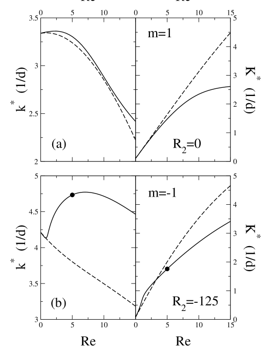
Figure 4: Evolution of the coordinates $k^{\ast}$ and $K^{\ast}$ of the saddle point that determines the boundary, $R_{1c-a}$, between convective and absolute instability with through-flow Reynolds number $Re$. Full (dotted) lines are evaluated with the correct NSE (approximate GLE) dispersion relation. Filled circles in (b) at $Re=5$ mark the coordinates of the saddle in Fig. 5. The radius ratio is $\eta=0.5$.

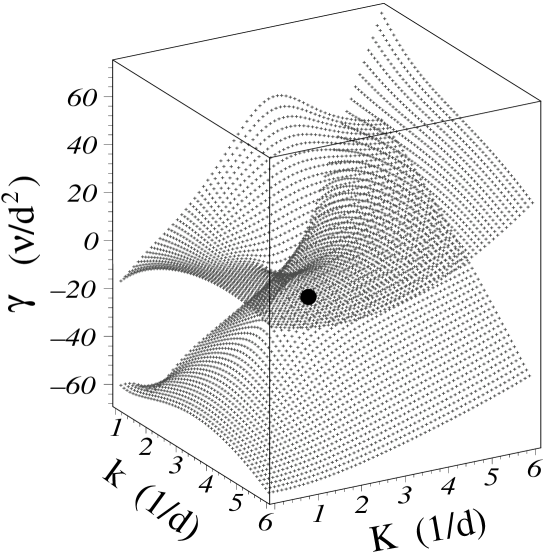
Figure 5: Real parts $\gamma(Q)$ of the two biggest eigenvalues of the NSE over the complex $Q-$plane for $m=-1$, $R_{2}=-125$, $Re=5$, $\mu=\mu_{c-a}$, $\eta=0.5$. The filled circle marks the saddle at $\gamma(Q^{\ast})=0$ that determines the boundary beteen convective and absolute instability.

It is remarkable that based on the experimental observations of Takeuchi and Jankowski TAK-JAN such a behavior was discussed already in 1979 [cf. figures 4 and 5(a) and their discussion in Sec. 6 of ref. TAK-JAN ], albeit without invoking the concept of absolute and convective instability b&b which was introduced to a broader fluid dynamics community only a few years later HUE .

IV.2 Boundary between convective and absolute instability: saddle point analysis

The boundary between convective and absolute instability of the basic flow against growth of vortices with a particular azimuthal wave number $m$ is marked by those parameter combinations for which one of the fronts of the linear packet of $m$-vortices reverts its propagation direction in the laboratory frame: In the convectively unstable parameter regime this front propagates in the same direction as the center of the packet, in the absolutely unstable regime it moves opposite to it, and right on the boundary between the two regimes the front is stationary in the laboratory frame.

This parameter combination can be determined by a saddle point analysis of the linear complex dispersion relation $\sigma(Q)$ over the plane of complex wave numbers HUE ; CRO-HOH

$$Q=\Re Q+i\Im Q=k-iK\,.$$ (44)

Here we do not display the dependence of

$$\sigma(Q)=\Re\sigma(Q)+i\Im\sigma(Q)=\gamma(Q)-i\omega(Q)$$ (45)

on the parameters $R_{1},R_{2},Re,\eta$ and we also do not indicate that the dispersion relations for vortex perturbations with different azimuthal wave numbers $m$ are different. The boundary condition of no growth for a front that is stationary in the laboratory system is

$$\Re\sigma=0$$ (46)

at the appropriate saddle position, $Q^{\ast}$, of $\sigma(Q)$ in the complex wave number plane HUE . Here $Q^{\ast}$ follows from

$$\frac{d\sigma(Q)}{dQ}\Big{|}_{Q^{\ast}}=0.$$ (47)

For fixed $m,R_{2},Re,\eta$ eqs.(46,47) yield $R_{1c-a}$. Here and in the following the subscript $c-a$ identifies boundaries between convective and absolute instability. Thus, e.g., the basic flow state is convectively [absolutely] unstable against vortex perturbations with azimuthal wave number $m$ for $R_{1c}(m)<R_{1}<R_{1c-a}(m)$ [$R_{1}>R_{1c-a}(m)$] and absolutely stable when $R_{1}<R_{1c}(m)$.

We are interested here in the $Re$ dependence of these thresholds and we will discuss to that end the reduced boundary quantities

$$\mu_{c-a}(Re)=\frac{R_{1c-a}(Re)}{R_{1c}(Re)}-1$$ (48)

and

$$\epsilon_{x}(Re)=\frac{R_{1x}(Re)}{R_{1c}(Re=0)}-1,\ \textrm{where}\ x=c\ \textrm{or}\ x=c-a\,.$$ (49)

Because of the symmetries of $\sigma(Q)$, of its saddle-point $Q^{\ast}$, and of the resulting boundary $R_{1c-a}(m,Re)$ one has

$$k^{\ast}(-m,-Re) = k^{\ast}(m,Re)$$ (50)

$$K^{\ast}(-m,-Re) = -K^{\ast}(m,Re)$$ (51)

$$\mu_{c-a}(-m,-Re) = \mu_{c-a}(m,Re)$$ (52)

$$\epsilon_{c-a}(-m,-Re) = \epsilon_{c-a}(m,Re)$$ (53)

so that it suffices again to investigate only positive through-flow.

IV.3 Numerical procedures

In order to determine the boundary between convective and absolute instability via the solution of eqs. (46, 47) one has to evaluate the dispersion relation $\sigma(Q)$ for complex $Q$ TAG-EDW-SWI ; BAC-Pre94 . To that end we solved the eigenvalue problem (28) of the full field equations for complex $Q$ (cf., Sec. IV.3.2). In addition and for comparison we used for $\sigma(Q)$ the Ginzburg-Landau amplitude equation approximation which only requires knowledge of $\sigma(k)$ along the real $k$-axis.

IV.3.1 Ginzburg-Landau amplitude equation approximation

Within this approximation the dispersion relation $\sigma(Q)$ for vortex modes is expanded in $Q$ and $R_{1}$ around the critical point $k_{c},R_{1c}$

$$\sigma(Q,R_{1}) = \sigma_{c}+\left(\frac{\partial\sigma}{\partial Q}\right)_{c}(Q-k_{c})+\frac{1}{2}\left(\frac{\partial^{2}\sigma}{\partial Q^{2}}\right)_{c}(Q-k_{c})^{2}$$ (55)

$$+\left(\frac{\partial\sigma}{\partial R_{1}}\right)_{c}(R_{1}-R_{1c})+h.o.t.$$

$$= -i\omega_{c}-iv_{g}(Q-k_{c})-\frac{\xi_{0}^{2}}{\tau_{0}}(1+ic_{1})(Q-k_{c})^{2}$$

$$+\frac{(1+ic_{0})}{\tau_{0}}\mu+h.o.t.\,.$$

The expansion coefficients in the above expressions appear also in the linear parts of the Ginzburg-Landau amplitude equation CRO-HOH . They are obtained from the numerical solution of the eigenvalue problem (28) of the full field equations for real $k$ close to the critical point REC-LUE-MUE ; PIN .

Within the GLE approximation one gets from eqs. (46, 47)

$$Q^{\ast}=\underbrace{k_{c}-\frac{c_{1}\tau_{0}v_{g}}{2(1+c_{1}^{2})\xi_{0}^{2}}}_{k^{\ast}}-i\underbrace{\frac{\tau_{0}v_{g}}{2(1+c_{1}^{2})\xi_{0}^{2}}}_{K^{\ast}},$$ (56)

$$\mu_{c-a}=\frac{v_{g}^{2}\tau_{0}^{2}}{4(1+c_{1}^{2})\xi_{0}^{2}},$$ (57)

and

$$\epsilon_{c-a}(Re)=\epsilon_{c}(Re)+\frac{v_{g}^{2}\tau_{0}^{2}}{4(1+c_{1}^{2})\xi_{0}^{2}}\left[1+\epsilon_{c}(Re)\right].$$ (58)

Note that the GLE coefficients $v_{g},\tau_{0},\xi_{0},c_{0},c_{1}$ depend on $m,R_{2},Re,\eta$. For $m=0$ and $R_{2}=0$ also the nonlinear coefficients of the GLE have been obtained for several $\eta$ as functions of $Re$ REC-LUE-MUE .

IV.3.2 Dispersion relation $\sigma(Q)$ of the NSE for complex $Q$

To assess the quality of the GLE results for the boundary between convective and absolute instability we determined the dispersion relation of the NSE not only for real $k$ close to the critical point but for complex axial wave numbers $Q$ that lie in the vicinity of the relevant saddle locations $Q^{\ast}$ of $\sigma(Q)$. Having determined $\sigma(Q)$ as described in Sec. II.4 we solved the equations (46,47) for $R_{1c-a}$ in the form

$$\gamma(Q^{\ast})=0;\quad\frac{\partial\gamma(Q)}{\partial K}\Big{|}_{Q^{\ast}}=0;\quad\frac{\partial\gamma(Q)}{\partial k}\Big{|}_{Q^{\ast}}=0$$ (59)

that follows from using the Cauchy-Riemann relations for $\sigma(Q)$.

IV.4 Results

In Fig. 4 we show the $Re$-variation of the real and imaginary parts of the relevant saddle-point $Q^{\ast}=k^{\ast}-iK^{\ast}$ at the boundary $R_{1c-a}$ for two characteristic cases: (a) L-SPI ($m=1$) at $R_{2}=0$ and (b) R-SPI ($m=-1$) at $R_{2}=-125$. In each case full (dashed) lines were obtained from the correct NSE (approximate GLE) dispersion relation $\sigma(Q)$.

Case (a) is representative for a situation where the GLE approximation reasonably well reproduces the correct result – at least for small $Re$ – and starts to deviate significantly only for larger $Re$. On the other hand, in case (b) the GLE approximation to $k^{\ast}$ displays a smooth variation with $Re$ that reflects the smooth variation of the saddle $Q^{\ast}_{GLE}$ (56) of $\sigma_{GLE}(Q)$ (55) while the real part $k^{\ast}$ of the saddle location of the correct dispersion relation undergoes a dramatic change around $Re\simeq 0.8$. The reason is that the surfaces of $\gamma(Q)=\Re\sigma(Q)$ over the $Q$-plane for the two largest eigenvalues intersect and change their order along the $\gamma$ axis. Thus, the saddle that is relevant for the $c-a$ transition and that has the largest $\gamma$ value switches from one eigenvalue surface to another. Similarly the eigenvalue surface might have another saddle and their ordering in $\gamma$ changes. In contrast to that the GLE approximation produces only a single eigenvalue tracing out the smooth surface $\sigma_{GLE}(Q)$ (55).

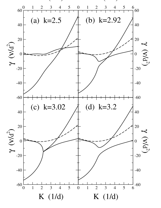
Figure 6: Full lines are sections through the surfaces of $\gamma(Q)$ (Fig. 5) for the two biggest eigenvalues of the NSE at constant values of $k$ in the vicinity of the intersection of the surfaces. Dashed lines show $\gamma(K)$ obtained from the GLE approximation to the dispersion relation. Parameters are $m=-1$, $R_{2}=-125$, $Re=5$, $\mu=\mu_{c-a}$, $\eta=0.5$.

To give an impression of such an intersection of the correct dispersion surfaces we show in Fig. 5 their real parts over the complex $Q-$plane at $Re=5,\mu=\mu_{c-a}$. Full lines in Fig. 6 show different constant-$k$ sections through them in the intersection range. At $Re=5,\mu=\mu_{c-a}$ the saddle has moved already away from the intersection region. The saddle coordinates ($Q^{\ast}\simeq 4.73-i1.76,\gamma^{\ast}=0$) are indicated in Figs. 4, 5 by full dots.

While the saddle locations $Q^{\ast}_{GLE}$ of the GLE approximation $\sigma_{GLE}(Q)$ (55) can differ substantially from the saddle $Q^{\ast}$ of the correct dispersion relation the difference in the boundaries between convective and absolute instability is typically much less pronounced – cf, e.g., the dashed and full curves for $\epsilon_{c-a}$ in Fig. 3. There the GLE results (dashed lines) agree in each case quite well with the correct boundaries (full lines) up to, say $Re=5$. However, as a consequence of the typical increase of the reduced boundary $\mu_{c-a}$ with increasing $Re$ the quality of the GLE results for $\mu_{c-a}$ generally deteriorates. After all the GLE is strictly valid only for $\mu\to 0$. Fig. 7 shows an example ($m=1,R_{2}=-125$) where the GLE prediction for the boundary shows even a qualitative different variation with $Re$ for, say, $Re>15$. We have observed similar behavior – partly at larger $Re$ – also for other combinations of $m,R_{2}$.

Tables 2 and 3 contain the coefficients for fitting our results for $\epsilon_{c-a}(m=0,R_{2},Re)$ and $\epsilon_{c-a}(m=1,R_{2},Re)$ in the same way as described in Sec. III.3. Also here the boundary curves for R-SPI $(m=-1)$ are obtained according to Sec. III.2 from those for L-SPI $(m=1)$ by $Re\rightarrow-Re$, i.e., by changing the sign of the odd coefficients in Table 3.

V Fronts and pulses

The vortex fronts that we are investigating here and that appear also as constituents of vortex pulses are perturbations of the basic state where the fields (locally) have the form

$$\psi\sim e^{i(k^{\ast}z-\omega^{\ast}t)}e^{K^{\ast}(z-v^{\ast}t)}e^{im\varphi}$$ (60)

in the laboratory frame. This form describes long-time spatiotemporal properties of uniquely selected linear fronts CRO-HOH . Axial front velocity $v^{\ast}$, axial growth rate $K^{\ast}$ of the front envelope, wave number $k^{\ast}$ of the vortex pattern under the front, and its frequency $\omega^{\ast}$ are determined by the saddle behavior of the linear complex dispersion relation $\sigma(Q,m)=\gamma(Q,m)-i\omega(Q,m)$ of the field equations over the plane of complex axial wave numbers $Q=k-iK$. Since superpositions of vortex perturbations with different $m$ evolve independently from each other within the linear description as mentioned already in Sec. IV.1 we consider here only fronts of vortex perturbations that have a common azimuthal wave number $m$ and we do not always display the latter explicitly.

The saddle condition is CRO-HOH

$$\frac{d}{dQ}\left[\sigma\left(Q\right)\>\>+\>\>i\>v\>Q\right]\Big{|}_{Q=Q^{\ast}}=0.$$ (61)

And the stationarity requirement that the temporal growth rate of the front vanishes in the frame comoving with the front velocity $v^{\ast}$ demands that

$$0=\Re\left[\sigma(Q)+ivQ\right]\Big{|}_{Q=Q^{\ast}}=\gamma(Q^{\ast})+v^{\ast}K^{\ast}.$$ (62)

We combine (61) and (62) into the three equations

$$v^{\ast}=-\frac{\gamma(Q^{\ast})}{K^{\ast}}=-\frac{\partial\gamma(Q)}{\partial K}\Big{|}_{Q^{\ast}}\quad;\quad\frac{\partial\gamma(Q)}{\partial k}\Big{|}_{Q^{\ast}}=0$$ (63)

that we have solved for $v^{\ast},k^{\ast},K^{\ast}$.

V.1 Notation

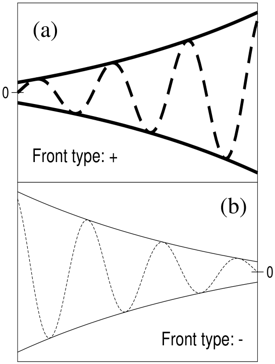
Figure 8: Schematic plot of different vortex fronts. Thick full lines in (a) and thin full lines in (b) show intensity envelopes of $+$ type and of $-$ type fronts connecting to the basic state at $z\to-\infty$ and at $z\to\infty$, respectively. This line convention — thick ones for $+$ type fronts and thin ones for $-$ type fronts — is used also in Fig. 9. Dashed lines indicate the vortex field growing under the front.

The front envelope of (60) varies axially with $e^{K^{\ast}z}$. If $K^{\ast}>0$, then the perturbation grows at $z=-\infty$ out of the basic state. We call such a front to be of type $+$ and identify the associated front properties by a subscript $+$. On the other hand, for $K^{\ast}<0$ we have a front of type $-$ with an intensity envelope that joins at $z=\infty$ with the basic state. So the two subscripts $\pm$ identify the axial variations of the front envelopes. A pulse-like perturbation of the basic state would consist suffiently away from its center of a $+$ front for $z\to-\infty$ and of a $-$ front for $z\to\infty$. Correspondingly the eqs. (63) have two different solutions: one of them describes a $-$ front and the other one a $+$ front. A schematic plot of the different envelope types can be seen in Fig. 8.

We identify the vortex pattern that is unfolded under a front either by its azimuthal wave number $m$ or by the superscripts T, L, R. Here T refers to a TVF-like pattern of vortices with $m=0$, L denotes L-spiral vortices with $m=1$, and R identifies R-spiral vortices with $m=-1$. Hence $m$ or equivalently the superscripts identify the spatiotemporal structure of the vortex pattern growing under the front. In this work we restrict ourselves to these three vortex varieties. Since they appear under the above described two front envelopes there are six different fronts that we have investigated here.

V.2 Results

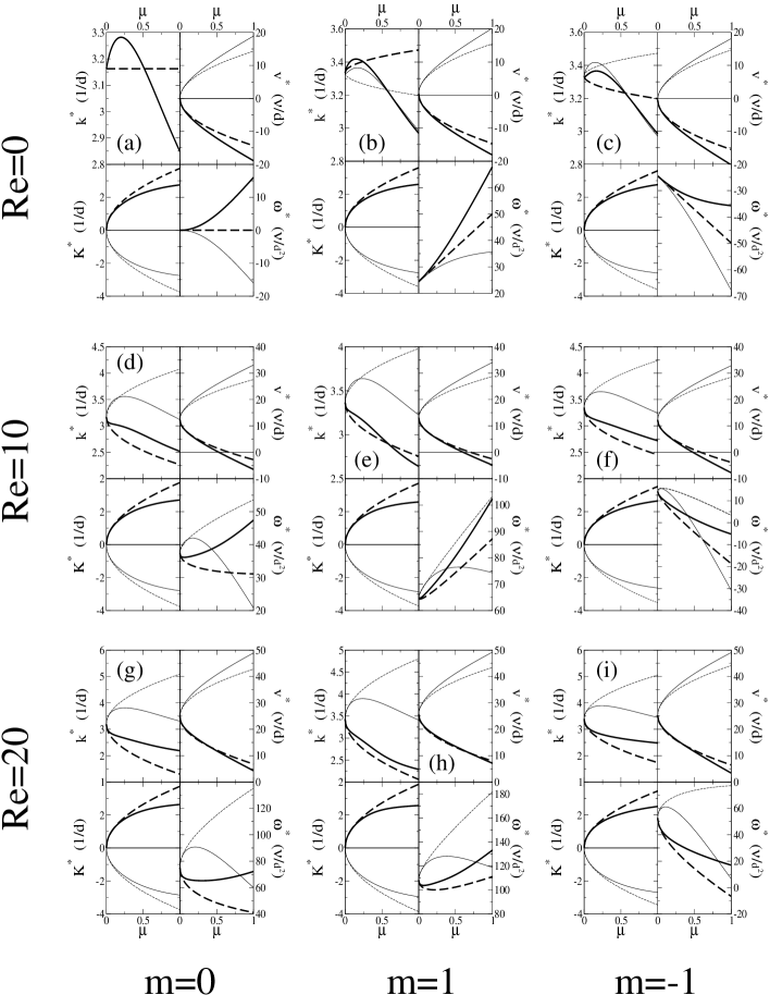
Figure 9: Front properties of vortices with azimuthal wave numbers $m=0,1,-1$ in systems with and without through-flow $Re$ for $R_{2}$ = 0, $\eta=0.5$ as functions of $\mu=R_{1}/R_{1c}(Re)-1$. Within each 2$\times$2 block of figures (a)-(i) the left column shows the axial wave number $k^{\ast}$ and the axial growth rate $K^{\ast}$. The right column shows the front velocity $v^{\ast}$ and the frequency $\omega^{\ast}$ in the laboratory frame. Thick lines correspond to $+$ fronts, thin lines to $-$ fronts, respectively. Full (dashed) lines result from the saddle point analysis of the dispersion relation of the NSE (GLE approximation).

In Fig. 9 the results of our investigations are shown for fronts with azimuthal wave numbers $m$ = 0, 1, and -1 for axial through-flow Reynolds numbers $Re$ =0, 10, and 20. In each case the outer cylinder is at rest, $R_{2}=0$. The front properties are presented as functions of $\mu$. Within each 2$\times$2 block of figures (a)-(i) the left column shows real part $k^{\ast}$ and negative imaginary part $K^{\ast}$ of the saddle point and the right column shows the front velocity $v^{\ast}$ and the frequency $\omega^{\ast}$, respectively. They all start at $\mu=0$ since vortex growth is possible only above the critical threshold, i.e., for $R_{1}>R_{1c}(Re)$. The two critical fronts at this threshold are degenerate ($k^{\ast}_{-}=k^{\ast}_{+}=k_{c},\,\omega^{\ast}_{-}=\omega^{\ast}_{+}=\omega_{c},\,v^{\ast}_{-}=v^{\ast}_{+}=v_{g}$) with vanishing axial growth rates $K^{\ast}_{-}=K^{\ast}_{+}=0$. For $\mu>0$, however, $+$ and $-$ fronts differ from each other thus reflecting differences in the respective saddle points.

The variation of $k^{\ast},K^{\ast},v^{\ast}$, and $\omega^{\ast}$ with $\mu$ and $Re$ is best understood by comparison with the corresponding GLE approximation (cf. Sec. V.2.1) and by invoking symmetry relations (cf. Sec. V.2.2). We therefore continue the discussion of our results in the following two sections V.2.1 and V.2.2.

V.2.1 Ginzburg-Landau amplitude equation approximation

The saddle point analysis (61 - 63) of the GLE approximation (55) yield the following front properties

$$K^{\ast}_{\pm} = \pm\sqrt{\frac{\mu}{(1+c_{1}^{2})\xi_{0}^{2}}},$$ (64)

$$k^{\ast}_{\pm} = k_{c}-c_{1}K^{\ast}_{\pm},$$ (65)

$$v^{\ast}_{\pm} = v_{g}-2(1+c_{1}^{2})\frac{\xi_{0}^{2}}{\tau_{0}}K^{\ast}_{\pm},$$ (66)

$$\gamma^{\ast}_{\pm} = -v^{\ast}_{\pm}K^{\ast}_{\pm},$$ (67)

$$\omega^{\ast}_{\pm} = \omega_{c}+v_{g}(k^{\ast}_{\pm}-k_{c})+(c_{1}-c_{0})\frac{\mu}{\tau_{0}}\,.$$ (68)

for the two fronts with $K_{+}^{\ast}>0$ and $K_{-}^{\ast}<0$, respectively. All quantities appearing in (64 - 68) depend on whether they refer to T ($m$ = 0), L ($m$ = 1), or R ($m$ = -1) vortex fronts. These GLE results are shown in Fig. 9 by dashed lines.

They reasonably well describe the small-$\mu$ behavior of the correct front properties (full lines in Fig. 9) which were obtained from the correct dispersion relation of the NSE: As predicted by the small-$\mu$ GLE approximation (64 - 68) one finds that for small $\mu$ the axial growth rates $K^{\ast}$ vary $\propto\sqrt{\mu}$, that consequently also $k^{\ast}-k_{c}$ and $v^{\ast}-v_{g}$ vary $\propto\sqrt{\mu}$, and that $\omega^{\ast}-\omega_{c}$ can have in addition also a contribution $\propto\mu$ when $c_{1}-c_{0}\neq 0$. The latter is the case for $m=\pm 1$ irrespective of $Re$ and for $m=0$ if $Re\neq 0$.

Note that for TVF fronts with $m=0,Re=0$ the GLE predicts $\omega^{\ast}=0$ whereas the correct dispersion in Fig. 9(a) seems to show for small $\mu$ a variation of $\omega^{\ast}\propto\mu^{2}$ that is beyond the range of applicability of the GLE. Thus, under the linear part of a moving TVF front there should be a non zero phase propagation in the laboratory frame with phase velocity $\omega^{\ast}/k^{\ast}$. The analogous behavior was found also for convection rolls in the Rayleigh-Bénard system BUE-LUE .

At the boundary between convective and absolute instability, $\mu=\mu_{c-a}$, the velocity $v_{+}^{\ast}$ and the temporal growth rate $\gamma^{\ast}_{+}$ of the $+$ front vanish in the laboratory frame while $v_{-}^{\ast}$ is positive there (and given by 2 $v_{g}$ within the GLE approximation). Note that according to Fig. 3 and tables 2 and 3 $\mu_{c-a}$ is zero for $m=0,Re=0$ and very small for $m=\pm 1,Re=0$. Only for large enough through-flow $\mu_{c-a}$ becomes sizeable. In the convectively unstable regime $0<\mu<\mu_{c-a}$ both, the $+$ front as well as the $-$ front of a vortex pulse move into the same downstream direction as the through-flow, $0<v_{+}^{\ast}<v_{-}^{\ast}$. In the absolutely unstable regime $\mu>\mu_{c-a}$, however, the $+$ front moves upstream and the $-$front moves downstream, $v_{+}^{\ast}<0<v_{-}^{\ast}$.

In ref. NG-TUR it was remarked that the phase velocity of spiral patterns in axial flow through a system of radius ratio $\eta=0.95$ SNY deviates from the critical one, $\omega_{c}/k_{c}$, of axially extended vortex perturbations. While we have done only calculations for $\eta=0.5$ our results of Fig. 9 and of the small-$\mu$ GLE approximation (64 - 68) shed some light on the existence of such deviations. Since the experimental vortex structures grow in downstream direction under intensity fronts one strictly speaking would have to compare with the phase velocity under such fronts that connect in the absolutely unstable regime to the fully developed downstream vortex pattern. Such a nonlinear analysis has been done for $m=0$ patterns BLRS96 but not for spirals. However, already the phase velocities $\omega_{+}^{\ast}/k_{+}^{\ast}$ under our linear $+$ fronts that grow in downstream direction differ from the corresponding critical phase velocities $\omega_{c}/k_{c}$ of axially extended patterns — cf. Fig. 9 and eqs. (64 - 68).

V.2.2 Symmetries

The front properties shown in Fig. 9 are largely influenced by the symmetry properties of the system without through-flow although a finite $Re$ changes them.

Invariance of the field equations under $z\to-z$ for $Re=0$ implies that stationary perturbations with $\omega_{c}=0$ (TVF) under a $+$ front are mirror images of those under a $-$ front. This implies for $Re=0$ the symmetry relations

$$(K,\omega,v)_{+}^{\ast T}=-(K,\omega,v)_{-}^{\ast T};\quad k_{+}^{\ast T}=k_{-}^{\ast T}.$$ (69)

These symmetry properties of the two front types of T-perturbations can be seen in Fig. 9(a).

Now consider L and R perturbations. Here the invariance of the field equations under $z\to-z$ for $Re=0$ implies first of all that a spatially extended L-SPI with uniform amplitude is the mirror image of a spatially extended R-SPI. Furthermore, a L-SPI under a $+$ front with positive $K$ is symmetry degenerate with a R-SPI under a $-$ front with negative $K$. Similarly a R-SPI under a $+$ type front is the mirror image of a L-SPI under a $-$ front. This implies for $Re=0$ the symmetry relations

$$(K,\omega,v)_{+}^{*L}=-(K,\omega,v)_{-}^{*R};\quad k_{+}^{*L}=k_{-}^{*R},$$ (70)

$$(K,\omega,v)_{+}^{\ast R}=-(K,\omega,v)_{-}^{\ast L};\quad k_{+}^{\ast R}=k_{-}^{\ast L}.$$ (71)

They can be seen to be realized in Fig. 9(b) and Fig. 9(c).

The GLE approximation (64) - (68) shows beyond the relations (69)-(71) the following additional relations

$$k_{+}^{\ast T}=k_{-}^{\ast T}=k_{c}^{T}\quad;\quad\omega_{+}^{\ast T}=\omega_{-}^{\ast T}=0$$ (72)

$$K_{+}^{\ast L}=-K_{-}^{\ast L}=K_{+}^{\ast R}=-K_{-}^{\ast R},$$ (73)

$$\omega_{+}^{\ast L}=\omega_{-}^{\ast L}=-\omega_{+}^{\ast R}=-\omega_{-}^{\ast R}$$ (74)

that follow from the fact, that $\omega_{c}^{T}=v_{g}^{T}=c_{0}^{T}=c_{1}^{T}=0$, $k_{c}^{R}=k_{c}^{L}$, $v_{g}^{R}=-v_{g}^{L}$, $\tau_{0}^{R}=\tau_{0}^{L}$, $c_{0}^{R}=-c_{0}^{L}$, $c_{1}^{R}=-c_{1}^{L}$, and $\xi_{0}^{R}=\xi_{0}^{L}$ for $Re=0$ PIN .

VI Summary

We have determined the influence of an axial through-flow on the spatiotemporal growth behavior of structurally different vortex perturbations of the basic Couette-Poiseuille flow in the Taylor-Couette system with radius ratio $\eta=0.5$. To that end we have solved the linearized NSE numerically with a shooting method for vortex perturbations with azmuthal wave numbers $m=0$ (TVF), $m=1$ (L-SPI), and $m=-1$ (R-SPI) in a wide range of the parameters $Re,R_{1}$, and $R_{2}$. Here symmetry properties allowed us to restrict ourselves to positive through-flow Reynolds numbers $Re$. For each of the three different vortex varieties we have investigated (i) axially extended vortex structures with homogeneous amplitudes, (ii) axially localized vortex pulses consisting of a linear superposition of axially extended vortex modes with different real axial wave numbers $k$, and (iii) vortex fronts.

Central to our analysis is the determination of the complex dispersion relations $\sigma(Q)$ of the linearized NSE for vortex modes with the three different $m$. We have evaluated $\sigma$ over the plane of complex wave numbers $Q=k-iK$ for patterns (ii, iii) and along the real $k$-axis for pattern (i). We have also determined the Ginzburg-Landau amplitude equation approximation $\sigma_{GLE}(Q)$ in order to analyze its predictions for the vortex stuctures (ii, iii) in comparison with the correct NSE dispersion relation $\sigma(Q)$. In each case symmetry relations are elucidated.

First we have evaluated the critical bifurcation thresholds $R_{1c}(Re,R_{2},m)$ for axially extended vortex structures. Then using a saddle-point analysis of $\sigma(Q)$ we have determined the boundaries $R_{1c-a}(Re,R_{2},m)$ between absolute and convective instability of the basic state at which one of the fronts of the expanding vortex pulses reverts its propagation direction in the laboratory frame. Here we have elucidated also in some detail how the different saddle topologies of $\sigma(Q)$ and of $\sigma_{GLE}(Q)$ explain some of the shortcomings of the latter. Fit parameters for power-law expansions of the reduced boundaries $\epsilon_{c},\epsilon_{c-a}$, and $\epsilon_{c-a}^{GLE}$ up to $Re^{4}$ are listed in two tables.

Finally we have determined the linearly selected front behavior of growing vortex patterns with $m=0,\pm 1$ for $R_{2}=0$ under two different types of front intensity envelopes: type $+$ shows growth in positive z-direction while type $-$ locates growth in negative z-direction. The combination of the three different dynamics of the constituent vortex modes ($m=0,\pm 1$) and of the two different spatial intensity profiles ($+$, $-$) leads to six different fronts $\sim e^{i(k^{\ast}z-\omega^{\ast}t)}e^{K^{\ast}(z-v^{\ast}t)}$ in the laboratory frame. Their velocity $v^{\ast}$, spatial growth rate $K^{\ast}$, wave number $k^{\ast}$, and frequency $\omega^{\ast}$ as determined via a saddle point analysis of the respective dispersion relations differ in general from each other in the presence of a through-flow.

Figure 7: Stability boundaries of the basic flow state as functions of the through-flow Reynolds number $Re$ for $m=1$, $R_{2}=-125$. The full (dashed) boundary lines, $\epsilon_{c-a}$, between the convectively and absolutely unstable parameter regions for vortex growth were obtained from the eigenvalues of the full NSE (the GLE approximation) – cf. Sec. IV. Dotted lines show the reduced critical bifurcation thresholds $\epsilon_{c}$ (4) for axially extended vortex patterns. The radius ratio is $\eta=0.5$.

	Operation
	A	B	C	D
$k\rightarrow$	$\quad k$	$\ -k$	$\ -k$	$\quad k$
$m\rightarrow$	$\quad m$	$\ -m$	$\quad m$	$\ -m$
$Re\rightarrow$	$\quad Re$	$\quad Re$	$\ -Re$	$\ -Re$
$\sigma\rightarrow$	$\quad\sigma$	$\quad{\overline{\sigma}}$	$\quad\sigma$	$\quad{\overline{\sigma}}$
$U\rightarrow$	$\quad U$	$\quad{\overline{U}}$	$\quad U$	$\quad{\overline{U}}$
$V\rightarrow$	$\quad V$	$\quad{\overline{V}}$	$\quad V$	$\quad{\overline{V}}$
$W\rightarrow$	$\quad W$	$\quad{\overline{W}}$	$\ -W$	$\ -{\overline{W}}$
$X\rightarrow$	$\quad X$	$\quad{\overline{X}}$	$\quad X$	$\quad{\overline{X}}$
$Y\rightarrow$	$\quad Y$	$\quad{\overline{Y}}$	$\quad Y$	$\quad{\overline{Y}}$
$Z\rightarrow$	$\quad Z$	$\quad{\overline{Z}}$	$\ -Z$	$\ -{\overline{Z}}$

Table 1: Transformation behavior of the eigenvalues and eigenfunctions of the eigenvalue problem (28 - 31) under symmetry operations. Here A denotes the identity, B complex conjugation, C axial reflection, and D complex conjugation (indicated by an overbar) combined with axial reflection.

$R_{2}$	-150	-125	-100	-75	-50	-25	0	25	50
$\epsilon_{c}=a_{2}Re^{2}+a_{4}Re^{4}$
$a_{2}*10^{4}$	0.590	0.795	1.089	1.502	2.083	3.115	3.679	2.447	1.307
$a_{4}*10^{9}$	5.181	3.966	1.151	-2.804	-3.385	-15.62	-34.97	-14.55	-0.958
$\epsilon_{c-a}=a_{2}Re^{2}+a_{4}Re^{4}$
$a_{2}*10^{3}$	1.181	1.451	1.854	2.516	3.906	5.588	6.238	4.338	2.483
$a_{4}*10^{6}$	0.116	0.139	0.182	0.293	-2.583	-4.642	-5.716	-3.682	-1.740
$\epsilon_{c-a}^{GLE}=a_{2}Re^{2}+a_{4}Re^{4}$
$a_{2}*10^{3}$	1.161	1.416	1.800	2.517	4.068	6.547	7.732	5.152	2.762
$a_{4}*10^{6}$	-0.164	-0.268	-0.481	-1.011	-2.106	-3.807	-4.900	-3.022	-1.425

Table 2: Fitparameters for the $Re$-dependence of the stability boundaries of the basic state against growth of TVF $(m=0)$ perturbations for different $R_{2}$: reduced critical bifurcation threshold $\epsilon_{c}$ of axially extended vortex patterns and boundary $\epsilon_{c-a}$ between convectively and absolutely unstable parameter regime. Here $\epsilon_{c-a}^{GLE}$ is obtained from the GLE approximation (cf. Sec. IV.3.1).

$R_{2}$	-150	-125	-100	-75	-50	-25	0	25	50
$\epsilon_{c}=a_{1}Re+a_{2}Re^{2}+a_{3}Re^{3}+a_{4}Re^{4}$
$a_{1}*10^{3}$	-1.582	-2.365	-3.513	-4.887	-6.143	-5.833	-3.372	-1.402	-0.514
$a_{2}*10^{4}$	0.957	1.199	1.496	1.925	2.520	3.174	3.197	1.806	0.581
$a_{3}*10^{7}$	-9.181	-9.001	-8.485	-7.678	-6.741	-4.172	-3.832	-3.572	-3.685
$a_{4}*10^{9}$	1.018	-0.378	-0.180	-0.563	-3.673	-21.77	-36.15	-5.707	19.92
$\epsilon_{c-a}=a_{0}+a_{1}Re+a_{2}Re^{2}+a_{3}Re^{3}+a_{4}Re^{4}$
$a_{0}*10^{3}$	2.358	5.497	3.775	-1.237	4.095	12.25	18.96	10.09	2.610
$a_{1}*10^{3}$	-3.268	-3.578	-3.048	-0.449	0.926	1.159	1.012	1.217	1.455
$a_{2}*10^{3}$	1.532	1.964	2.618	3.539	4.351	5.535	6.036	4.357	2.603
$a_{3}*10^{6}$	8.408	11.87	14.97	9.992	6.487	4.919	3.680	1.367	-0.143
$a_{4}*10^{6}$	-0.169	-0.368	-0.815	-1.977	-2.809	-4.068	-4.827	-3.203	-1.549
$\epsilon_{c-a}^{GLE}=a_{0}+a_{1}Re+a_{2}Re^{2}+a_{3}Re^{3}+a_{4}Re^{4}$
$a_{0}*10^{3}$	1.101	-2.541	1.405	2.529	3.458	3.998	3.641	1.320	0.062
$a_{1}*10^{3}$	-4.117	0.755	-1.044	-0.318	0.831	2.063	1.495	1.377	1.625
$a_{2}*10^{3}$	2.030	2.792	2.820	3.435	4.437	6.166	7.265	4.981	2.723
$a_{3}*10^{6}$	-8.845	-30.34	-7.121	4.780	10.58	8.229	-8.191	-12.58	-10.03
$a_{4}*10^{6}$	-0.822	-2.713	-1.136	-1.004	-1.674	-2.923	-3.799	-2.234	-0.854

Table 3: Fitparameters for the $Re$-dependence of the stability boundaries of the basic state against growth of L-SPI $(m=1)$ perturbations for different $R_{2}$: reduced critical bifurcation threshold $\epsilon_{c}$ of axially extended vortex patterns and boundary $\epsilon_{c-a}$ between convectively and absolutely unstable parameter regime. Here $\epsilon_{c-a}^{GLE}$ is obtained from the GLE approximation (cf. Sec. IV.3.1). The results for R-SPI $(m=-1)$ perturbations are obtained according to Sec. III.2 from those for L-SPI $(m=1)$ by $Re\rightarrow-Re$, i.e., by changing the sign of the odd coefficients in the table.