Induced-charge electro-osmosis

Abstract

We describe the general phenomenon of ‘induced-charge electro-osmosis’ (ICEO) — the nonlinear electro-osmotic slip that occurs when an applied field acts on the ionic charge it induces around a polarizable surface. Motivated by a simple physical picture, we calculate ICEO flows around conducting cylinders in steady (DC), oscillatory (AC), and suddenly-applied electric fields. This picture, and these systems, represent perhaps the clearest example of nonlinear electrokinetic phenomena. We complement and verify this physically-motivated approach using a matched asymptotic expansion to the electrokinetic equations in the thin double-layer and low potential limits. ICEO slip velocities vary like $u_{s}\propto E_{0}^{2}L$, where $E_{0}$ is the field strength and $L$ is a geometric length scale, and are set up on a time scale $\tau_{c}=\lambda_{D}L/D$, where $\lambda_{D}$ is the screening length and $D$ is the ionic diffusion constant. We propose and analyze ICEO microfluidic pumps and mixers that operate without moving parts under low applied potentials. Similar flows around metallic colloids with fixed total charge have been described in the Russian literature (largely unnoticed in the West). ICEO flows around conductors with fixed potential, on the other hand, have no colloidal analog and offer further possibilities for microfluidic applications.

1 Introduction

Recent developments in micro-fabrication and the technological promise of microfluidic ‘labs on a chip’ have brought a renewed interest to the study of low-Reynolds number flows ([Stone & Kim (2001), Whitesides & Stroock (2001), Reyes et al. (2002)]). The familiar techniques used in larger-scale applications for fluid manipulation, which often exploit fluid instabilities due to inertial nonlinearities, do not work on the micron scale due to the pre-eminence of viscous damping. The microscale mixing of miscible fluids must thus occur without the benefit of turbulence, by molecular diffusion alone. For extremely small devices, molecular diffusion is relatively rapid; however, in typical microfluidic devices with 10-100 $\mu$m features, the mixing time can be prohibitively long (of order 100 s for molecules with diffusivity $10^{-10}$ m²/s). Another limitation arises because the pressure-driven flow rate through small channels decreases with the third or fourth power of channel size. Innovative ideas are thus being considered for pumping, mixing, manipulating and separating on the micron length scale (e.g. [Beebe et al. (2002), Whitesides et al. (2001)]). Naturally, many focus on the use of surface phenomena, owing to the large surface to volume ratios of typical microfluidic devices.

Electrokinetic phenomena provide one of the most popular non-mechanical techniques in microfluidics. The basic idea behind electrokinetic phenomena is as follows: locally non-neutral fluid occurs adjacent to charged solid surfaces, where a diffuse cloud of oppositely-charged counter-ions ‘screen’ the surface charge. An externally-applied electric field exerts a force on this charged diffuse layer, which gives rise to a fluid flow relative to the particle or surface. Electrokinetic flow around stationary surfaces is known as electro-osmotic flow, and the electrokinetic motion of freely-suspended particles is known as electrophoresis. Electro-osmosis and electrophoresis find wide application in analytical chemistry ([Bruin (2000)]), genomics ([Landers (2003)]) and proteomics ([Figeys & Pinto (2001), Dolnik & Hutterer (2001)]).

The standard picture for electrokinetic phenomena involves surfaces with fixed, constant charge (or, equivalently, zeta potential $\zeta$, defined as the potential drop across the screening cloud). Recently, variants on this picture have been explored. [Anderson (1985)] demonstrated that interesting and counter-intuitive effects occur with spatially inhomogeneous zeta-potentials, and showed that the electrophoretic mobility of a colloid was sensitive to the distribution of surface charge, rather than simply the total net charge. [Anderson & Idol (1985)] explored electro-osmotic flow in inhomogeneously-charged pores, and found eddies and recirculation regions. Ajdari (1995; 2001) and [Stroock et al. (2000)] showed that a net electro-osmotic flow could be driven either parallel or perpendicular to an applied field by modulating the surface and charge density of a microchannel, and [Gitlin et al. (2003)] have implemented these ideas to make a ‘transverse electrokinetic pump’. Such transverse pumps have the advantage that a strong field can be established with a low voltage applied across a narrow channel. [Long & Ajdari (1998)] examined electrophoresis of patterned colloids, and found example colloids whose electrophoretic motion is always transverse to the applied electric field. Finally, [Long et al.(1999)], [Ghosal (2003)], and others have studied electro-osmosis along inhomogeneously-charged channel walls (due to, e.g. , adsorption of analyte molecules), which provides an additional source of dispersion that can limit resolution in capillary electrophoresis.

Other variants involve surface charge densities that are not fixed, but rather are induced (either actively or passively). For example, the effective zeta potential of channel walls can be manipulated using an auxillary electrode to improve separation efficiency in capillary electrophoresis ([Lee et al. (1990), Hayes & Ewing (1992)]) and, by analogy with the electronic field-effect transistor, to set up ‘field-effect electro-osmosis’ ([Ghowsi & Gale (1991), Gajar & Geis (1992), Schasfoort et al. (1999)]).

Time-varying, inhomogeneous charge double-layers induced around electrodes give rise to interesting effects as well. [Trau et al. (1997)] and [Yeh et al. (1997)] demonstrated that colloidal spheres can spontaneously self-assemble into crystalline aggregates near electrodes under AC applied fields. They proposed somewhat similar electrohydrodynamic mechanisms for this aggregation, in which an inhomogeneous screening cloud is formed by (and interacts with) the inhomogeneous applied electric field (perturbed by the sphere), resulting in a rectified electro-osmotic flow directed radially in toward the sphere. More recently, [Nadal et al. (2002a)] performed detailed measurements in order to test both the attractive (electrohydrodynamic) and repulsive (electrostatic) interactions between the spheres, and [Ristenpart et al. (2003)] explored the rich variety of patterns that form when bidisperse colloidal suspensions self-assemble near electrodes.

A related phenomenon allows steady electro-osmotic flows to be driven using AC electric fields. Ramos et al. (1998; 1999) and [Gonzalez et al. (2000)] theoretically and experimentally explored ‘AC electro-osmosis’, in which a pair of adjacent, flat electrodes located on a glass slide and subjected to AC driving, gives rise to a steady electro-osmotic flow consisting of two counter-rotating rolls. Around the same time, [Ajdari (2000)] theoretically predicted that an asymmetric array of electrodes with applied AC fields generally pumps fluid in the direction of broken symmetry (‘AC pumping’). [Brown et al. (2001)], [Studer et al. (2002)], and [Mpholo et al. (2003)] have since developed AC electrokinetic micro-pumps based on this effect, and [Ramos et al. (2003)] have furthered their analysis.

Both AC colloidal self-assembly and AC electro-osmosis occur around electrodes whose potential is externally controlled. Both effects are strongest when the voltage oscillates at a special AC frequency (the inverse of the charging time discussed below), and both effects disappear in the DC limit. Furthermore, both vary with the square of the applied voltage $V_{0}$. This nonlinear dependence can be understood qualitatively as follows: the induced charge cloud/zeta potential varies linearly with $V_{0}$, and the resulting flow is driven by the external field, which also varies with $V_{0}$. On the other hand, DC colloidal aggregation, as explored by [Solomentsev et al. (1997)], requires large enough voltages to pass a Faradaic current, and is driven by a different, linear mechanism.

Very recently in microfluidics, a few cases of non-linear electro-osmotic flows around isolated and inert (but polarizable) objects have been reported, with both AC and DC forcing. In a situation reminiscent of AC electro-osmosis, [Nadal et al. (2002b)] studied the micro-flow produced around a dielectric stripe on a planar blocking electrode. In rather different situations, [Thamida & Chang (2002)] observed a DC nonlinear electrokinetic jet directed away from a protruding corner in a dielectric microchannel, far away from any electrode, and [Takhistov et al. (2003)] observed electrokinetically driven vortices near channel junctions. These studies (and the present work) suggest that a rich variety of nonlinear electrokinetic phenomena at polarizable surfaces remains to be exploited in microfluidic devices.

In colloidal science, nonlinear electro-osmotic flows around polarizable (metallic or dielectric) particles were studied almost two decades ago in a series of Ukrainian papers, reviewed by [Murtsovkin (1996)], that has gone all but unnoticed in the West. Such flows occur when the applied field acts on the component of the double-layer charge that has been polarized by the field itself. This idea can be traced back at least to [Levich (1962)], who discussed the dipolar charge double layer (using the Helmholtz model) that is induced around a metallic colloidal particle in an external electric field and touched upon the quadrupolar flow that would result. [Simonov & S. S. Dukhin (1973)] calculated the structure of the (polarized) dipolar charge cloud in order to obtain the electrophoretic mobility, without concentrating on the resulting flow. [Gamayunov, Murtsovkin & A. S. Dukhin (1986)] and [A. S. Dukhin & Murtsovkin (1986)] first explicitly calculated the nonlinear electro-osmotic flow arising from double-layer polarization around a spherical conducting particle, and [A. S. Dukhin (1986)] extended this calculation to include a dielectric surface coating (as a model of a dead biological cell). Experimentally, [Gamayunov et al. (1992)] observed a non-linear flow around spherical metallic colloids, albeit in a direction opposite to predicitions for all but the smallest particles. They argued that a Faradaic current (breakdown of ideal polarizibility) was responsible for the observed flow reversal.

This work followed naturally from many earlier studies on ‘non-equilibrium electric surface phenomena’ reviewed by [S. S. Dukhin (1993)], especially those focusing on the ‘induced dipole moment’ (IDM) of a colloidal particle reviewed by [S. S. Dukhin & Shilov (1980)]. Following [Overbeek (1943)], who was perhaps the first to consider non-uniform polarization of the double layer in the context of electrophoresis, [S. S. Dukhin (1965)], [S. S. Dukhin & Semenikhin (1970)], and [S. S. Dukhin & Shilov (1974)] predicted the electrophoretic mobility of a highly charged non-polarizable sphere in the thin double-layer limit, in good agreement with the later numerical solutions of [O’Brien & White (1978)]. (See, e.g., [Lyklema (1991)].) In that case, diffuse charge is redistributed by surface conduction, which produces an IDM aligned with the field and some variations in neutral bulk concentration, and secondary electro-osmotic and diffusio-osmotic flows develop as a result. [Shilov & S. S. Dukhin (1970)] extended this work to a non-polarizable sphere in an AC electric field. [Simonov & S. S. Dukhin (1973)] and [Simonov & Shilov (1973)] performed similar calculations for an ideally polarizable, conducting sphere, which typically exhibits an IDM opposite to the applied field. [Simonov & Shilov (1977)] revisited this problem in the context of dielectric dispersion and proposed a much simpler RC-circuit model to explain the sign and frequency dependence of the IDM. [O’Brien & White (1978)] performed a numerical solution of the full ion, electrostatic, and fluid equations with arbitrarily thick double-layer, which naturally incorporated the effects of double-layer polarization. [O’Brien & Hunter (1981)] and [O’Brien (1983)], following Dukhin’s approach, arrived at a simpler, approximate expression that incorporated double-layer polarization in the thin double-layer limit, and compared favorably with the numerical calculations of [O’Brien & White (1978)]. Nonetheless, it seems a detailed study of the associated electro-osmotic flows around polarizable spheres did not appear until the paper of [Gamayunov, Murtsovkin & A. S. Dukhin (1986)] cited above.

In summary, we note that electrokinetic phenomena at polarizable surfaces share a fundamental feature: all involve a nonlinear flow component in which double-layer charge induced by the applied field is driven by that same field. To emphasize this common mechanism, we suggest the term ‘induced-charge electro-osmosis’ (ICEO) for their description. Specific realizations of ICEO include AC electro-osmosis at micro-electrodes, AC pumping by asymmetric electrode arrays, DC electrokinetic jets around dielectric structures, DC and AC flows around polarizable colloidal particles, and the situations described below. Of course, other electrokinetic effects may also occur in addition to ICEO in any given system, such as those related to bulk concentration gradients produced by surface conduction or Faradaic reactions, but we ignore such complications here to highlight the basic effect of ICEO.

In the present work, we build upon this foundation of induced-charge electrokinetic phenomena, with a specific eye towards microfluidic applications. ICEO flows around metallic colloids, which have attraced little attention compared to non-polarizable objects of fixed zeta potential, naturally lend themselves for use in microfluidic devices. In that setting, the particle is replaced by a fixed polarizable object which pumps the fluid in response to applied fields, and a host of new possibilities arise. The ability to directly control the position, shape, and potential of one or more ‘inducing surfaces’ in a microchannel allows for a rich variety of effects that do not occur in colloidal systems.

Before we begin, we note the difference between ICEO and ‘electrokinetic phenomena of the second kind’, reviewed by [S. S. Dukhin (1991)] and studied recently by [Ben & Chang (2002)] in the context of microfluidic applications. Significantly, second-kind electrokinetic effects do not arise from the double-layer, being instead driven by space charge in the bulk solution. They typically occur around ion-selective porous granules subject to applied fields large enough to generate strong currents of certain ions through the liquid/solid interface. This leads to large concentration variations and space charge in the bulk electrolyte on one side, which interact with the applied field to cause motion. [Barany et al. (1998)] studied the analogous effect for non-porous metallic colloids undergoing electrochemical reactions at very large Faradaic currents (exceeding diffusion limitation). In contrast, ICEO occurs around inert polarizable surfaces carrying no Faradaic current in contact with a homogeneous, quasi-neutral electrolyte and relies on relatively small induced double-layer charge, rather than bulk space charge.

The article is organized as follows: §2 provides a basic background on electrokinetic effects, and §3 develops a basic physical picture of induced-charge electro-osmosis via calculations of steady ICEO flow around a conducting cylinder. §4 examines the time-dependent ICEO flow for background electric fields which are suddenly-applied (§4.1) or sinusoidal (§4.2). §5 describes some basic issues for ICEO in microfluidic devices, such as coupling to the external circuit (§5.1) and the phenomenon of fixed-potential ICEO (§5.2). Some specific designs for microfluidic pumps, junction switches, and mixers are discussed and analyzed in §5.3. §6 investigates the detrimental effect of a thin dielectric coating on a conducting surface and calculates the ICEO flow around non-conducting dielectric cylinders. §7 gives a systematic derivation of ICEO in the limit of thin double layers and small potentials, starting with the basic electrokinetic equations and employing matched asymptotic expansions, concluding with a set of effective equations (with approximations and errors quantified) for the ICEO flow around an arbitrarily-shaped particle in an arbitrary space- and time-dependent electric field. The interesting consequences of shape and field asymmetries, which generally lead to electro-osmotic pumping or electrophoretic motion in AC fields, are left for a companion paper. The reader is referred to [Bazant & Squires (2004)] for an overview of our results.

2 Classical (‘fixed-charge’) electro-osmosis

Electrokinetic techniques provide some of the most popular small-scale non-mechanical strategies for manipulating particles and fluids. We present here a very brief introduction. More detailed accounts are given by [Lyklema (1991)], [Hunter (2000)] and [Russel et al. (1989)].

Figure 1: Left: A charged solid surface in an electrolytic solution attracts an oppositely-charged ‘screening cloud’ of width $\sim\lambda_{D}$. An electric field applied tangent to the charged solid surface gives rise to an electro-osmotic flow (4). Right: An electric field applied to an electrolytic solution containing a suspended solid particle gives rise to particle motion called electrophoresis, with velocity equal in magnitude and opposite in direction to (4).

2.1 Small zeta potentials

A surface with charge density $q$ in an aqueous solutions attracts a screening cloud of oppositely-charged counter-ions to form the electrochemical ‘double layer’, which is effectively a surface capacitor. In the Debye-Hückel limit of small surface charge, the excess diffuse ionic charge exponentially screens the electric field set up by the surface charge (figure 1a), giving an electrostatic potential

$$\phi=\frac{q}{\varepsilon_{w}\kappa}e^{-\kappa z}\equiv\zeta e^{-\kappa z}.$$ (1)

Here $\varepsilon_{w}\approx 80\varepsilon_{0}$ is the dielectric permittivity of the solvent (typically water) and $\varepsilon_{0}$ is the vacuum permittivity. The ‘zeta potential’, defined by

$$\zeta\equiv\frac{q}{\varepsilon_{w}\kappa},$$ (2)

reflects the electrostatic potential drop across the screening cloud, and the Debye ‘screening length’ $\kappa^{-1}$ is defined for a symmetric $z$:$z$ electrolyte by

$$\kappa^{-1}\equiv\lambda_{D}=\sqrt{\frac{\varepsilon_{w}k_{B}T}{2n_{0}(ze)^{2}}},$$ (3)

with bulk ion concentration $n_{0}$, (monovalent) ion charge $e$, Boltzmann constant $k_{B}$ and temperature $T$. Because the ions in the diffuse part of the double layer are approximately in thermal equilibrium, the condition for a ‘small’ charge density (or zeta potential) is $\zeta\ll k_{B}T/ze$.

An externally applied electric field exerts a body force on the electrically charged fluid in this screening cloud, driving the ions and the fluid into motion. The resulting electro-osmotic fluid flow (figure 1a) appears to ‘slip’ just outside the screening layer of width $\lambda_{D}$. Under a wide range of conditions, the local slip velocity is given by the Helmholtz-Smoluchowski formula,

$${\bf u}_{s}=-\frac{\varepsilon_{w}\zeta}{\eta}{\bf E}_{||},$$ (4)

where $\eta$ is the fluid viscosity and ${\bf E}_{||}$ is the tangential component of the bulk electric field.

This basic electrokinetic phenomenon gives rise to two related effects, electro-osmosis and electrophoresis, both of which find wide application in analytical chemistry, microfluidics, colloidal self-assembly, and other emerging technologies. Electro-osmotic flow occurs when an electric field is applied along a channel with charged walls, wherein the electro-osmotic slip at the channel walls gives rise to plug flow in the channel, with velocity given by (4). Because the electro-osmotic flow velocity is independent of channel size, (in contrast to pressure-driven flow, which depends strongly upon channel size), electro-osmotic pumping presents a natural and popular technique for fluid manipulation in small channels. On the other hand, when the solid/fluid interface is that of a freely-suspended particle, the electro-osmotic slip velocity gives rise to motion of the particle itself (figure 1b), termed electrophoresis. In the thin double-layer limit, the electrophoretic velocity is given by Smoluchowski’s formula,

$${\bf U}=\frac{\varepsilon_{w}\zeta}{\eta}{\bf E}_{\infty}\equiv\mu_{e}{\bf E}_{\infty},$$ (5)

where ${\bf E}_{\infty}$ is the externally-applied field, and $\mu_{e}=\varepsilon_{w}\zeta/\eta$ is the electrophoretic mobility of the particle.

2.2 Large zeta potentials

For ‘large’ zeta potentials, comparable to or exceeding $k_{B}T/ze$, the exponential profile of the diffuse charge (1) and the linear charge-voltage relation (2) are no longer valid, but the diffuse part of the double layer remains in thermal equilibrium. As a result, the potential in the diffuse layer satisfies the Poisson-Boltzmann equation. For symmetric, binary electrolyte, the classical Gouy-Chapman solution yields a nonlinear charge-voltage relation for the double layer,

$$q(\zeta)=4n_{0}ze\lambda_{D}\,\sinh\left(\frac{ze\zeta}{2k_{B}T}\right),$$ (6)

in the thin double-layer limit. This relation may be modified to account for microscopic surface properties, such as a compact Stern layer, a thin dielectric coating, or Faradaic reactions, which enter via the boundary conditions to the Poisson-Boltzmann equation. The key point here is simply that $q$ generally grows exponentially with $ze\zeta/k_{B}T$, which has important implications for time-dependent problems involving double-layer relaxation, as reviewed by [Bazant, Thornton & Ajdari (2004)].

Remarkably, the Helmholtz-Smoluchowski formula (4) for the electro-osmotic slip remains valid in the nonlinear regime, as long as

$$\frac{\lambda_{D}}{a}\,\exp\left(\frac{ze\zeta}{2k_{B}T}\right)\ll 1,$$ (7)

where $a$ is the radius of curvature of the surface (Hunter 2000). When (7) is violated, ionic concentrations in the diffuse layer differ significantly from their bulk values, and surface conduction through the diffuse layer becomes important. As a result, the electrophoretic mobility, $\mu_{e}$, becomes a nonlinear function of the dimensionless ratio

$$\mbox{Du}=\frac{\sigma_{s}}{\sigma a},$$ (8)

of the surface conductivity, $\sigma_{s}$, to the bulk conductivity, $\sigma$. Though this ratio was first noted by [Bikerman (1940)], we follow [Lyklema (1991)] in referring to (8) as the ‘Dukhin number’, in honor of Dukhin’s pioneering calculations of its effect on electrophoresis. We note also that essentially the same number has been called $\alpha$, $\beta$, and $\lambda$ by various authors in the Western literature, and ‘${\rm Rel}$’ by [S. S. Dukhin (1993)].

Bikerman (1933; 1935) made the first theoretical predictions of surface conductance, $\sigma_{s}$, taking into account both electromigration and electro-osmosis in the diffuse layer. The relative importance of the latter is determined by another dimensionless number

$$m=\left(\frac{k_{B}T}{ze}\right)^{2}\frac{2\varepsilon_{w}}{\eta D}.$$ (9)

Using the result of [Deryagin & S. S. Dukhin (1969)], Bikerman’s formula for $\sigma_{s}$ takes a simple form for a symmetric binary electrolyte, yielding

$$\mbox{Du}=\frac{2\lambda_{D}(1+m)}{a}\left[\cosh\left(\frac{ze\zeta}{2k_{B}T}\right)-1\right]=4\frac{\lambda_{D}(1+m)}{a}\sinh^{2}\left(\frac{ze\zeta}{4k_{B}T}\right)$$ (10)

for the Dukhin number. In the limit of infinitely thin double layers, where (7) holds, the Dukhin number vanishes, and the electrophoretic mobility tends to Smoluchowski’s value (4). For any finite double-layer thickness, however, highly charged particles (with $\zeta>k_{B}T/ze$) are generally described by a non-negligible Dukhin number, and surface conduction becomes important. This leads to bulk concentration gradients and a non-uniform diffuse-charge distribution around the particle in an applied field, which modifies its electrophoretic mobility, via diffusiophoresis and concentration polarization. For more details, the reader is referred to [Lyklema (1991)] and [S. S. Dukhin (1993)].

3 Induced-charge electro-osmosis: fundamental picture

The standard electrokinetic picture described above involves the interaction of an applied field and a surface of fixed charge, wherein the electro-osmotic flow is linear in the applied field. Here we focus on the nonlinear phenomenon of ICEO at a polarizable (metal or dielectric) surface. As a consequence of nonlinearity, ICEO can be used to drive steady electro-osmotic flows using AC or DC fields. The nonlinearity also allows for larger fluid velocities and a richer, geometry-dependent flow structure. These properties stand in stark contrast to classical electro-osmosis described above, which, e.g. , gives zero time-averaged flow in an AC field.

This section gives a physically clear (as well as quantitatively accurate) sense of ICEO in perhaps the simplest case: an ideally polarizable metal cylinder in a suddenly applied, uniform electric field. This builds on the descriptions of double-layer polarization for an uncharged metallic sphere by [Levich (1962)], [Simonov & Shilov (1973)] and [Simonov & Shilov (1977)] and the associated steady ICEO flow by [Gamayunov, Murtsovkin & A. S. Dukhin (1986)]. We postpone for §7 a more detailed and general analysis, justifying the approximations made here for the case of thin double layers ($\lambda_{D}\ll a$) and weak applied fields ($E_{0}a\ll k_{B}T/ze$). Since $\mbox{Du}\ll 1$ in these limits, surface conduction and concentration polarization can be safely ignored, and ICEO becomes the dominant electrokinetic effect around any inert, highly polarizable object.

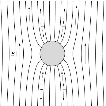
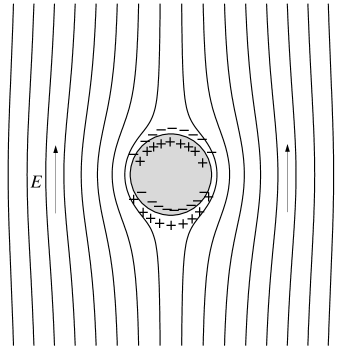
Figure 2: The evolution of the electric field around a solid, ideally polarizable conducting cylinder immersed in a liquid electrolyte, following the imposition of a background DC field at $t=0$ (a), where the field lines intersect normal to the conducting surface. Over a charging time $\tau_{c}=\lambda_{D}a/D$, a dipolar charge cloud forms in response to currents from the bulk, reaching steady state (b) when the bulk field profile is that of an insulator. The resulting zeta potential, however, is nonuniform.

Figure 3: The steady-state induced-charge electro-osmotic flow around (a) a conducting cylinder with zero net charge and (b) a positively charged conducting cylinder. The ICEO slip velocity depends on the product of the steady field and the induced zeta potential. The flow around an uncharged conducting cylinder (a) can thus be understood qualitatively from figure 2b, whereas the charged sylinder (b) simply involves the superposition of the standard electro-osmotic flow.

3.1 Steady ICEO around an uncharged conducting cylinder

The basic phenomenon of ICEO can be understood from figures 2 and 3. Immediately after an external field ${\bf E}=E_{0}{\bf{\hat{z}}}$ is applied, an electric field is set up so that field lines intersect conducting surfaces at right angles (figure 2a). Although this represents the steady-state vacuum field configuration, mobile ions in electrolytic solutions move in response to applied fields. A current $\mbox{\bf J}=\sigma{\bf E}$ drives positive ions into a charge cloud on one side of the conductor ($z<0$), and negative ions to the other ($z>0$), inducing an equal and opposite surface charge on the conducting surface. A dipolar charge cloud grows so long as a normal field injects ions into the induced double layer, and steady state is achieved when no field lines penetrate the double-layer (figure 2b). The tangential field $E_{||}$ drives an electro-osmotic slip velocity (4) proportional to the local double-layer charge density, driving fluid from the ‘poles’ of the particle towards the ‘equator’ (figure 3a). An AC field drives an identical flow, since an oppositely-directed field induces an oppositely-charged screening cloud, giving the same net flow. The ICEO flow around a conducting cylinder with non-zero total charge, shown in figure 3b, simply superimposes the nonlinear ICEO flow of figure 3a with the usual linear electro-osmotic flow.

As a concrete example for quantitative analysis, we consider an isolated, uncharged conducting cylinder of radius $a$ submerged in an electrolyte solution with very small screening length $\lambda_{D}\ll a$. An external electric field $E_{0}{\bf{\hat{z}}}$ is suddenly applied at $t=0$, and the conducting surface forms an equipotential surface, giving a potential

$$\phi_{0}=-E_{0}z\left(1-\frac{a^{2}}{r^{2}}\right).$$ (11)

Electric field lines intersect the conducting surface at right angles, as shown in figure 2a.

Due to the electrolyte’s conductivity $\sigma$, a non-zero current $\mbox{\bf J}=\sigma{\bf E}$ drives ions to the cylinder surface. In the absence of electrochemical reactions at the conductor/electrolyte interface (i.e. at sufficiently low potentials that the cylinder is ‘ideally polarizable’), mobile solute ions accumulate in a screening cloud adjacent to the solid/liquid surface, attracting equal and opposite ‘image charges’ within the conductor itself. Thus the conductor’s surface charge density $q$ — induced by the growing screening cloud — changes in a time-dependent fashion, via

$$\frac{dq(\theta)}{dt}={\bf j}\cdot{\bf{\hat{r}}}=\sigma{\bf E}\cdot{\bf{\hat{r}}}.$$ (12)

Using the linear relationship (2) between surface charge density and zeta potential, this can be expressed as

$$\frac{d\zeta(\theta)}{dt}=\frac{\sigma}{\varepsilon_{w}\kappa}{\bf E}\cdot{\bf{\hat{r}}}.$$ (13)

A dipolar charge cloud grows, since positively-charged ions are driven into the charge cloud on the side of the conductor nearest the field source ($z<0$ in this case), and negatively-charged ions are driven into the charge cloud on the opposite side. As ions are driven into the screening charge cloud, field lines are expelled and the ionic flux into the charge cloud is reduced.

The system reaches a steady state configuration when all field lines are expelled (${\bf{\hat{r}}}\cdot{\bf E}(a)=0$). This occurs when the electrostatic potential outside of the charge cloud is given by

$$\phi_{f}=-E_{0}z\left(1+\frac{a^{2}}{r^{2}}\right),$$ (14)

shown in figure 2b. The steady-state electrostatic configuration is thus equivalent to the no-flux electrostatic boundary condition assumed in the analysis of ‘standard’ electrophoresis. In the present case, however, the steady-state configuration corresponds to a cylinder whose zeta potential varies with position according to

$$\zeta(\theta)=\phi_{o}-\phi_{f}(a)=2E_{0}a\cos\theta,$$ (15)

where we assume the conductor potential $\phi_{o}$ to vanish. While the steady-state electric field has no component normal to the charge cloud, its tangential component,

$${\bf{\hat{\theta}}}\cdot{\bf E}=-2E_{0}\sin\theta,$$ (16)

drives an induced-charge electro-osmotic flow, with slip velocity given by (4). Now, however, the (spatially-varying) surface potential $\zeta$ is given by (15). Because the charge cloud is itself dipolar, the tangential field drives the two sides of the charge cloud in opposite directions—each side away from the poles—resulting in a quadrupolar electro-osmotic slip velocity

$${\bf u}_{s}=2U_{0}\sin 2\theta\,\,{\bf{\hat{\theta}}},$$ (17)

where $U_{0}$ is the natural velocity scale for ICEO,

$$U_{0}=\frac{\varepsilon_{w}E_{0}^{2}a}{\eta}.$$ (18)

One power of $E_{0}$ sets up the ‘induced-charge’ screening cloud, and the second drives the resultant electro-osmotic flow.

The fluid motion in this problem is reminiscent of that around a fluid drop of one conductivity immersed in a fluid of another conductivity subjected to an external electric field, studied by [Taylor (1966)]. By analogy, we find the radial and azimuthal fluid velocity components of the fluid flow outside of the cylinder to be

$$u_{r}=2\frac{a(a^{2}-r^{2})}{r^{3}}U_{0}\cos 2\theta,\,\,\,\,\,\,u_{\theta}=2\frac{a^{3}}{r^{3}}U_{0}\sin 2\theta.$$ (19)

For comparison, analogous results for the steady-state ICEO flow around a sphere, some of which were derived by [Gamayunov, Murtsovkin & A. S. Dukhin (1986)], are given in Table 1.

	Cylinder	Sphere
Initial potential $\phi_{i}$	$-E_{0}z\left(1-\frac{a^{2}}{r^{2}}\right)$	$-E_{0}z\left(1-\frac{a^{3}}{r^{3}}\right)$
Steady-state potential $\phi_{s}$	$-E_{0}z\left(1+\frac{a^{2}}{r^{2}}\right)$	$-E_{0}z\left(1+\frac{a^{3}}{2r^{3}}\right)$
Steady-state zeta potential $\zeta$	$2E_{0}a\cos\theta$	$\frac{3}{2}E_{0}a\cos\theta$
Radial flow $u_{r}$	$\frac{2a(a^{2}-r^{2})}{r^{3}}U_{0}\cos 2\theta$	$\frac{9a^{2}(a^{2}-r^{2})}{16r^{4}}U_{0}\left(1+3\cos 2\theta\right)$
Azimuthal flow $u_{\theta}$	$\frac{2a^{3}}{r^{3}}U_{0}\sin 2\theta$	$\frac{9a^{4}}{8r^{4}}U_{0}\sin 2\theta$
Charging Timescale	$\tau_{c}=\frac{\lambda_{D}a}{D}$	$\tau_{s}=\frac{\lambda_{D}a}{D}$
Induced dipole strength:
$g(t)$ for suddenly applied field ${\bf E}_{0}$	$g(t)=1-2e^{-t/\tau_{c}}$	$g(t)=\frac{1}{2}\left(1-3e^{-2t/\tau_{s}}\right)$
$g$ for AC field $\mbox{Re}({\bf E}_{0}e^{i\omega t})$	$g=\frac{1-i\omega\tau_{c}}{1+i\omega\tau_{c}}$	$g=\frac{1-i\omega\tau_{s}}{2+i\omega\tau_{s}}$

Table 1: Electrostatic and hydrodynamic quantities for the induced-charge electro-osmotic (ICEO) flow around conducting spheres and cylinders, each of radius $a$. Here $U_{0}=\varepsilon_{w}E_{0}^{2}a/\eta$ is a characteristic velocity scale, and the induced dipole strength $g$ is defined in (23). See [Gamayunov, Murtsovkin & A. S. Dukhin (1986)] for flows around metal colloidal spheres in steady and AC fields.

Although we focus on the limit of linear screening in this paper, (19) should also hold for non-linear screening ($\zeta\approx k_{B}T/ze$) in the limit of thin double layers, as long as the Dukhin number remains small and (7) is satisfied. The relevant zeta potential in these conditions, however, is not the equilibrium zeta potential ($\zeta_{0}=0$) but the typical induced zeta potential, $\zeta\approx E_{0}a$, which is roughly the applied voltage across the particle.

Finally, although we have specifically considered a conducting cylinder, a similar picture clearly holds for more general shapes. More generally, ICEO slip velocities around arbitrarily-shaped inert objects in uniform applied fields are directed along the surface from the ‘poles’ of the object (as defined by the applied field), towards the object’s ‘equator’.

3.2 Steady ICEO around a charged conducting cylinder

Until now, we have assumed the cylinder to have zero net charge for simplicity. A cylinder with non-zero equilibrium charge density $q_{0}=Q/4\pi a^{2}$, or zeta potential, $\zeta_{0}=\varepsilon_{w}\kappa q_{0}$, in a suddenly applied field approaches a steady-state zeta-potential distribution,

$$\zeta(\theta)=\zeta_{0}+2E_{0}a\cos\theta,$$ (20)

which has the same induced component in (15) added to the constant equilibrium value. This follows from the linearity of (13) with the initial condition, $\zeta(\theta,t=0)=\zeta_{0}$. As a result, the steady-state electro-osmotic slip is simply a superposition of the ‘standard’ electro-osmotic flow due to the equilibrium zeta potential $\zeta_{0}$,

$${\bf u}_{s}^{Q}={\bf u}_{s}-2\frac{\varepsilon_{w}\zeta_{0}}{\eta}\sin\theta\,\,{\bf{\hat{\theta}}},$$ (21)

where ${\bf u}_{s}$ is the ICEO slip velocity, given in (17). The associated Stokes flow, which is a superposition of the ICEO flow and the ‘standard’ electro-osmotic flow, and is shown in figure 3(b).

The electrophoretic velocity of a charged conducting cylinder can be found using the results of [Stone & Samuel (1996)], from which it follows that the velocity of a cylinder with prescribed slip velocity ${\bf u}_{s}(\theta)$, but no externally-applied force, is given by the surface-averaged velocity,

$${\bf U}=-\frac{1}{2\pi}\int_{0}^{2\pi}{\bf u}_{s}(\theta)d\theta.$$ (22)

The ICEO component (17) has zero surface average, leaving only the ‘standard’ electro-osmotic slip velocity (21). This was pointed out by [Levich (1962)] using a Helmholtz model for the induced double layer, and later by [Simonov & S. S. Dukhin (1973)] using a double-layer structure found by solving the electrokinetic equations. The conducting cylinder thus has the same electrophoretic mobility $\mu_{e}=\varepsilon_{w}\zeta_{0}/\eta$ as an object of fixed uniform charge density and constant zeta potential. This extreme case illustrates the result of [O’Brien & White (1978)] that the electrophoretic mobility does not depend on electrostatic boundary conditions, even though the flow around the particle clearly does.

As above, the steady-state analysis of ICEO for a charged conductor is unaffected by nonlinear screening, as long as (7) is satisfied (and $\mbox{Du}\ll 1$), where the relevant $\zeta$ is the maximum value, $\zeta=|\zeta_{0}|+|E_{0}a|$, including both equilibrium and induced components.

4 Time-dependent ICEO

A significant feature of ICEO flow is its dependence on the square of the electric field amplitude. This has important consequences for AC fields: if the direction of the electric field in the above picture is reversed, so are the signs of the induced surface charge and screening cloud. The resultant ICEO flow, however, remains unchanged: the net flow generically occurs away from the poles, and towards the equator. Therefore, induced-charge electro-osmotic flows persist even in an AC applied fields, so long as the frequency is sufficiently low that the induced-charge screening clouds have time to form.

AC forcing is desirable in microfluidic devices, so it is important to examine the time-dependence of ICEO flows. As above, we explicitly consider a conducting (ideally polarizable) cylinder and simply quote the analogous results for a conducting sphere in Table 1. Although we perform calculations for the more tractable case of linear screening, we briefly indicate how the analysis would change for large induced zeta potentials. Two situations of interest are presented: the time-dependent response of a conducting cylinder to a suddenly-applied electric field (§4.1) and a sinusoidal AC electric field (§4.2). We also comment on the basic time scale for ICEO flows.

4.1 ICEO around a conducting cylinder in a suddenly-applied DC field

Consider first the time-dependent response of an uncharged conducting cylinder in an electrolyte when a uniform electric field ${\bf E}=E_{0}{\bf{\bf{\hat{z}}}}$ is suddenly turned on at $t=0$. The dipolar nature of the external driving suggests a bulk electric field of the form

$$\phi({\bf r},t)=-E_{0}z\left(1+g(t)\frac{a^{2}}{r^{2}}\right),$$ (23)

so that initially $g(0)=-1$ (11), and in steady state $g(t\rightarrow\infty)=1$ (14). The potential of the conducting surface itself remains zero, so that the potential drop across the double layer is given by

$$\phi(a,\theta,t)=-\zeta(\theta)=-\frac{q(\theta)}{\varepsilon_{w}\kappa}.$$ (24)

Here, as before, we take $q$ to represent the induced surface charge, so that the total charge per unit area in the charge cloud is $-q$. The electric field normal to the surface, found from (23), drives an ionic current

$$J_{\perp}=-\dot{q}(\theta)=-\sigma E_{0}\cos\theta\left(1-g\right),$$ (25)

into the charge cloud, locally injecting a surface charge density $\dot{q}$ per unit time. We express the induced charge density $q$ in terms of the induced dipole $g$ by substituting (23) into (24), take a time derivative, and equate the result with $\dot{q}$ given by (25). This results in an ordinary differential equation for the dipole strength $g$,

$$\dot{g}=\frac{\sigma}{\varepsilon_{w}\kappa a}(1-g),$$ (26)

whose solution is

$$g(t)=1-2e^{-t/\tau_{c}}.$$ (27)

Here $\tau_{c}$ is the characteristic time for the formation of induced-charge screening clouds,

$$\tau_{c}=\frac{\kappa a\varepsilon_{w}}{\sigma}=\frac{\lambda_{D}a}{D},$$ (28)

where the definitions of conductivity ($\sigma=2n_{0}e^{2}D/k_{B}T$) and screening length (3) have been used.

The induced-charge screening cloud (with equivalent zeta potential given by (24)) is driven by the tangential field (derived from (23)) in the standard way (4), resulting in an induced-charge electro-osmotic slip velocity

$${\bf u}_{s}=2U_{0}\sin 2\theta\left(1-e^{-t/\tau_{c}}\right)^{2}{\bf{\hat{\theta}}}.$$ (29)

More generally, the time-dependent slip velocity around a cylinder with a nonzero fixed charge (or equilibrium zeta potential $\zeta_{0}$) can be found in similar fashion, and results in the standard ICEO slip velocity ${\bf u}_{s}$ (29) with an additional term representing standard electro-osmotic slip (21)

$${\bf u}^{Q}_{s}={\bf u}_{s}-2\frac{\varepsilon_{w}\zeta_{0}}{\eta}\sin\theta\left(1-e^{-t/\tau_{c}}\right){\bf{\hat{\theta}}}.$$ (30)

Note that (30) grows more quickly than (29) initially, but that ICEO slip eventually dominates in strong fields, since it varies with $E_{0}^{2}$, versus $E_{0}$ for the standard electro-osmotic slip.

4.2 ICEO around a conducting cylinder in a sinusoidal AC field

An analogous calculation can be performed in a straightforward fashion for sinusoidal applied fields. Representing the electric field using complex notation, ${\bf E}=E_{0}e^{i\omega t}{\bf{\bf{\hat{z}}}},$ where the real part is implied, we obtain a time-dependent zeta potential

$$\zeta=2E_{0}a\cos\theta\,\mbox{Re}\,\,\left(\frac{e^{i\omega t}}{1+i\omega\tau_{c}}\right),$$ (31)

giving an induced-charge electro-osmotic slip velocity

$${\bf u}_{s}=2U_{0}\sin 2\theta\left[\mbox{Re}\left(\frac{e^{i\omega t}}{1+i\omega\tau_{c}}\right)\right]^{2}{\bf{\hat{\theta}}},$$ (32)

with time-averaged slip velocity

$$\langle{\bf u}_{s}\rangle=\frac{U_{0}\sin 2\theta}{(1+\omega^{2}\tau_{c}^{2})}{\bf{\hat{\theta}}}.$$ (33)

In the low-frequency limit $\omega\tau_{c}\ll 1$, the double-layer fully develops in phase with the applied field. In the high-frequency limit $\omega\tau_{c}\gg 1$, the double-layer does not have time to charge up, attaining a maximum magnitude $(\omega\tau_{c})^{-2}$ with a $\pi/2$ phase shift. Note that this analysis assumes that the double-layer changes quasi-steadily, which requires $\omega\ll\tau_{D}^{-1}.$

4.3 Time scales for ICEO flows

Before continuing, it is worth emphasizing the fundamental time scales arising in ICEO. The basic charging time $\tau_{c}$ exceeds the Debye time for diffusion across the double-layer thickness, $\tau_{D}=\lambda_{D}^{2}/D=\varepsilon_{w}/\sigma$, by a geometry-dependent factor, $a/\lambda_{D}$, that is typically very large. $\tau_{c}$ is also much smaller than the diffusion time across the particle, $\tau_{a}=a^{2}/D$. The appearance of this time scale for induced dipole moment of a metallic colloidal sphere has been explained by [Simonov & Shilov (1977)] using a simple RC-circuit analogy, consistent with the detailed analysis of [Simonov & Shilov (1973)]. The same time scale, $\tau_{c}$, also arises as the inverse frequency of AC electro-osmosis ([Ramos et al. (1999)]) or AC pumping ([Ajdari (2000)]) at a micro-electrode array of characteristic length $a$, where again an RC-circuit analogy has been invoked to explain the charging process. This simple physical picture has been criticized by [Scott et al. (2001)], but [Ramos et al. (2001)] and [Gonzalez et al. (2000)] have convincingly defended its validity, as in the earlier Russian papers on polarizable colloids.

Although it is apparently not well known in microfluidics and colloidal science, the time scale for double-layer relaxation was debated and analyzed in electrochemistry in the middle of the last century, after [Ferry (1948)] predicted that $\tau_{D}$ should be the charging-time for the double layer at an electrode in a semi-infinite electrochemical cell. [Buck (1969)] explicitly corrected Ferry’s analysis to account for bulk conduction, which introduces the macroscopic electrode separation $a$. The issue was definitively settled by [Macdonald (1970)] who explained the correct charging time, $\tau_{c}$, as the ‘$RC$ time’ for the double-layer capacitor, $C=\varepsilon_{w}/\lambda_{D}$, coupled to a bulk resistor, $R=a/\sigma$. Similiar ideas were also developed independently a decade later by [Kornyshev & Vorotyntsev (1981)] in the context of solid electrolytes.

Ferry’s model problem of a suddenly imposed surface charge-density in a semi-infinite electrolyte (as opposed to a suddenly imposed voltage or background field in a finite system) persists in recent textbooks on colloidal science, such as [Hunter (2000)] and [Lyklema (1991)], and only the time scales $\tau_{D}$ and $\tau_{a}$ are presented as relevant for double-layer relaxation. This is quite reasonable for non-polarizable colloidal particles, but we stress that the intermediate RC time scale, $\tau_{c}=\sqrt{\tau_{D}\tau_{a}}$, plays a central role for polarizable objects that exhibit significant double-layer charging.

We also mention nonlinear screening effects at large applied fields or large total charges, where the maximum total zeta potential, $\zeta\approx\zeta_{0}+E_{0}a$, exceeds $k_{B}T/ze$. The analysis of this section can be generalized to account for the ‘weakly nonlinear’ limit of thin double layers, where $\zeta>k_{B}T/ze$, but (7) is still satisfied (and thus $\mbox{Du}\ll 1$ as well). In the absence of surface conduction, (12) still describes double-layer relaxation, but a nonlinear charge-voltage relation, such as (6) from Gouy-Chapman theory, must be used. In that case, the time-dependent boundary condition (13) on the cylinder is replaced by

$$C_{D}(\zeta)\,\frac{d\zeta}{dt}=\sigma\,{\bf E}\cdot{\bf{\hat{r}}},$$ (34)

where

$$C_{D}(\zeta)=\frac{\varepsilon_{w}}{\lambda_{D}}\,\cosh\left(\frac{ze\zeta}{2k_{B}T}\right)$$ (35)

is the nonlinear differential capacitance of the double layer.

If the induced component of the zeta potential is large, due to a strong applied field, $E_{0}a>k_{B}T/ze$, the charging dynamics in (34) are no longer analytically tractable. Since the differential capacitance $C_{D}(\zeta)$ increases with $|\zeta|$ in any thin double-layer model, the ‘poles’ of the cylinder along the applied field charge more slowly than the sides. However, the steady-state field is the same as for linear screening, so long as $\mbox{Du}\ll 1$ .

If the applied field is weak, but the total charge is large ($\zeta_{0}>k_{B}T/ze$), (34) may be linearized to obtain the same polarization dynamics and ICEO flow as for $\mbox{Du}\ll 1$. However, the ‘$RC$ time’,

$$\tau_{c}(\zeta_{0})=R\,C_{D}=\tau_{c}\,\cosh\left(\frac{ze\zeta_{0}}{2k_{B}T}\right),$$ (36)

increases nonlinearly with $\zeta_{0}$, as shown by [Simonov & Shilov (1977)]. The same time constant, with $\zeta_{0}$ replaced by $\zeta_{0}+E_{0}a$, also describes the late stages of relaxation in response to a strong applied field.

Some implications for ICEO at large voltages in the ‘strongly nonlinear’ limit of thin double layers, where condition (7) is violated and $\mbox{Du}\gg 1$, are discussed in §7.5. In this regime, the simple circuit approximation breaks down due to bulk diffusion, and secondary relaxation occurs at the slow time scale, $\tau_{a}=a^{2}/D$. For an interdisciplinary review and detailed analysis of double-layer relaxation (without surface conduction or flow), the reader is referred to [Bazant, Thornton & Ajdari (2004)].

Finally, we note that the oscillatory component of ICEO flows may not obey the quasi-steady Stokes equations, due to the finite time scale, $\tau_{v}=a^{2}/\nu$, for the diffusion of fluid vorticity. (Here $\nu=\eta/\rho$ is the kinematic viscosity and $\rho$ the fluid density.) It is customary in microfluidic and colloidal systems to neglect the unsteady term, $\rho\partial{\bf u}/\partial t$, in the Stokes equations, because ions diffuse more slowly than vorticity by a factor of $D/\nu\approx 10^{-3}$. However, the natural time scale for the AC component of AC electro-osmotic flows is $\tau_{c}=\lambda_{D}a/D$, so the importance of the unsteady term in the Stokes equations is governed by the dimensionless parameter,

$$\frac{\tau_{v}}{\tau_{c}}=\frac{a}{\lambda_{D}}\,\frac{D}{\nu}.$$ (37)

This becomes significant for sufficiently thin double layers, $\lambda_{D}/a\approx 10^{-3}$. Therefore, in AC electro-osmosis and other ICEO phenomena with AC forcing at the charging frequency, $\omega_{c}=\tau_{c}^{-1}$, vorticity diffusion confines the oscillating component of ICEO flow to an oscillatory boundary layer of size $\sqrt{\nu\lambda_{D}a/D}$. However, the steady component of ICEO flows is usually the most important, and obeys the steady Stokes equations.

5 ICEO in microfluidic devices

We have thus far considered isolated conductors in background fields applied ‘at infinity’, as is standard in the colloidal context. The further richness of ICEO phenomena becomes apparent in the context of microfluidic devices. In this section, we consider ICEO in which the external field is applied by electrodes with finite, rather than infinite, separation. Furthermore, microfluidic devices allow additional techniques not available for colloids: the ‘inducing surface’ can be held in place and its potential can be actively controlled. This gives rise to ‘fixed-potential’ ICEO, which is to be contrasted with the ‘fixed-total-charge’ ICEO studied above. Finally, we present a series of simple ICEO-based microfluidic devices that operate without moving parts in AC fields.

5.1 Double-layer relaxation at electrodes

As emphasized above, one must drive a current $J_{0}(t)=\sigma E_{0}(t)$ to apply an electric field $E_{0}(t)$ in an homogeneous electrolyte. The electrochemical reactions associated with steady Faradaic currents may cause fluid contamination by reaction products or electrodeposits, unwanted concentration polarization, or permanent dissolution (and thus irreversible failure) of microelectrodes. Therefore, oscillating voltages and non-Faradaic displacement currents at ‘blocking’ electrodes are preferable in microfluidic devices. In this case, however, one must take care that diffuse-layer charging at the electrodes does not screen the field.

We examine the simplest case here, which involves a device consisting of a thin conducting cylinder of radius $a\gg\lambda_{D}$ placed between flat, inert electrodes separated by $2L\gg 2a$. The cylinder is electrically isolated from the rest of the system, so that its total charge is fixed. Under a suddenly applied DC voltage, $2V_{0}$, the bulk electric field, $E_{0}(t)$, decays to zero as screening clouds develop at the electrodes. For weak potentials ($V_{0}\ll k_{B}T/e$) and thin double-layers ($\lambda_{D}\ll a\ll L$), the bulk field decays exponentially

$$E_{0}(t)=\frac{V_{0}}{L}e^{-t/\tau_{e}},$$ (38)

with a characteristic electrode charging time

$$\tau_{e}=\frac{\lambda_{D}L}{D},$$ (39)

analogous to the cylinder’s charging time (28). This time-dependent field $E_{0}(t)$ then acts as the ‘applied field at infinity’ in the ICEO slip formula, (29).

The ICEO flow around the cylinder is set into motion exponentially over the cylinder charging time, $\tau_{c}=\lambda_{D}a/D$, but is terminated exponentially over the (longer) electrode charging time, $\tau_{e}=\lambda_{D}L/D$ as the bulk field is screened at the electrodes. This interplay between two time scales — one set by the geometry of the inducing surface and another set by the electrode geometry — is a common feature of ICEO in microfluidic devices.

This is clearly seen in the important case of AC forcing by a voltage, $V_{0}\cos(\omega t)$, in which the bulk electric field is given by

$$E_{0}(t)=\frac{V_{0}}{L}\mbox{Re}\left(\frac{i\omega\tau_{e}}{1+i\omega\tau_{e}}e^{-i\omega t}\right).$$ (40)

Electric fields persist in the bulk solution when the driving frequency is high enough $(\omega\tau_{e}\gg 1)$ that induced double-layers do not have time to develop near the electrodes. Induced-charge electro-osmotic flows driven by applied AC fields can thus persist only in a certain band of driving frequencies, $\tau_{e}^{-1}\leq\omega\leq\tau_{c}^{-1}$, unless Faradaic reactions occur at the electrodes to maintain the bulk field. In AC electro-osmosis at adjacent surface electrodes ([Ramos et al. (1999)]) or AC pumping at an asymmetric electrode array ([Ajdari (2000)]), the inducing surfaces are the electrodes, and so the two time scales coincide to yield a single characteristic frequency $\omega_{c}=1/\tau_{e}$. (Note that [Ramos et al. (1999)] and [Gonzalez et al. (2000)] use the equivalent form $\omega\sim\sigma\lambda_{D}/\varepsilon_{w}L$.)

Table 2 presents typical values for ICEO flow velocities and charging time scales for some reasonable microfluidic parameters. For example, an applied electric field of strength $100$ V/cm across an electrolyte containing a 10 $\mu$m cylindrical post gives rise to an ICEO slip velocity of order 1 mm/s, with charging times $\tau_{c}\sim 0.1$ ms and $\tau_{e}=0.1$ s.

Material properties of aqueous solution
Dielectric constant	$\varepsilon_{w}\approx 80\varepsilon_{0}$	$7\times 10^{-5}$	g cm/V2s2
Viscosity	$\eta$	$10^{-2}$	g/cm s
Ion Diffusivity	$D_{i}$	$10^{-5}$	cm2/s
Experimental Parameters
Screening Length	$\lambda_{D}$	10	nm
Cylinder radius	$a$	10	$\mu$m
Applied field	$E_{0}$	100	V/cm
Electrode Separation	$L$	1	cm
Characteristic Scales
Slip velocity	$U_{0}=\varepsilon_{w}E_{0}^{2}a/\eta$	0.7	mm/s
Cylinder charging time	$\tau_{c}$ = $\lambda_{D}a/D_{i}$	$10^{-4}$	s
Electrode charging time	$\tau_{e}$ = $\lambda_{D}L/D_{i}$	$10^{-1}$	s
Dimensionless Surface Potential	$\Psi$ = $eE_{0}a/k_{B}T$	3.9
Dukhin number	${\rm Du}$	$10^{-2}$

Table 2: Representative values for induced-charge electro-osmosis in a microfluidic device.

5.2 Fixed-potential ICEO

In the above examples, we have assumed a conducting element which is electrically isolated from the driving electrodes, which constrains the total charge on the conductor. Another possibility involves fixing the potential of the conducting surface with respect to the driving electrodes, which requires charge to flow onto and off of the conductor. This ability to directly control the induced charge allows for a wide variety of microfluidic pumping strategies exploiting ICEO.

Perhaps the simplest example of fixed-potential ICEO involves a conducting cylinder of radius $a$ which is held in place at a distance $h$ from the nearest electrode (figure 4a). For simplicity, we consider $a\ll h$ and $h\ll L$. We take the cylinder to be held at some potential $V_{c}$, the nearest electrode to be held at $V_{0}$, the other electrode at $V=0$, and assume the electrode charging time $\tau_{e}$ to be long. In this case, the bulk field (unperturbed by the conducting cylinder) is given simply by $E_{0}=V_{0}/L$, and the ‘background’ potential at the cylinder location is given by $\phi(h)=V_{0}(1-h/L)$. In order to maintain a potential $V_{c}$, an average zeta potential,

$$\zeta_{i}=V_{c}-V_{0}\left(1-\frac{h}{L}\right),$$ (41)

is induced via a net transfer of charge per unit length of $\lambda_{i}=2\pi\varepsilon_{w}\kappa a\zeta_{i}$, along with an equally and oppositely charged screening cloud.

This induced screening cloud is driven by the tangential electric field (16) in the standard way, giving a fixed-potential ICEO flow with slip velocity

$${\bf u}_{s}^{{\rm FP}}={\bf u}_{s}+2\frac{\varepsilon_{w}}{\eta}\frac{V_{0}}{L}\sin\theta\left(V_{c}-V_{0}+\frac{V_{0}h}{L}\right){\bf{\hat{\theta}}},$$ (42)

where ${\bf u}_{s}$ is the quadrupolar ‘fixed-total-charge’ ICEO flow ${\bf u}_{s}$ from (17) and (18), with $E_{0}=V_{0}/L$. Note that both the magnitude and direction of the flow can be controlled by changing the position $h$ or the potential $V_{c}$ of the inducing conductor. A freely-suspended cylinder would move with an electrophoretic velocity

$$U_{E}=\frac{dh}{dt}=\frac{\varepsilon_{w}}{\eta}\frac{V_{0}}{L}\left(V_{c}-V_{0}+\frac{V_{0}h}{L}\right)=\frac{h-h_{c}}{a}U_{0},$$ (43)

away from the position $h_{c}=L(1-V_{c}/V_{0})$ where its potential is equal to the (unperturbed) background potential. The velocity scale is the same as for fixed-total-charge ICEO, although the cylinder-electrode separation $h$, rather than the cylinder radius $a$, provides the geometric length scale. Since typically $h\gg a$, fixed-potential ICEO velocities are larger than fixed-total-charge ICEO for the same field.

Figure 4: Fixed-potential ICEO. a) A cylinder of radius $a$ is held a distance $h\gg a$ from a nearby electrode and held at the same electrostatic potential $V_{0}$ as the electrode. A second electrode is located a distance $L$ away and held at zero potential, so that a field $E_{0}\approx V_{0}/L$ is established. b) Leading-order fixed-potential ICEO flow for the system on the left. Like fixed-charge ICEO, a non-zero steady flow can be driven with an AC voltage.

To hold the cylinder in place against $U_{E}$, however, a force is required. Following [Jeffrey & Onishi (1981)], the force $F_{E}$ is given approximately by

$$F_{E}=\frac{4\pi\eta U_{E}}{\log\left[(h+\sqrt{h^{2}-a^{2}})/a\right]-\sqrt{h^{2}-a^{2}}/a}\approx\frac{4\pi\eta U_{E}}{\log\left(2h/a\right)-1},$$ (44)

and is directed toward $h_{c}$. The fixed-potential ICEO flow around a cylinder held in place at the same potential as the nearest electrode ($V_{c}=V_{0}$, $h_{c}=0$) is shown in figure 4. The leading-order flow consists of a Stokeslet of strength $F_{E}$ plus its images, following [Liron & Blake (1981)]. The (quadrupolar) fixed-total-charge ICEO flow exists in addition to the flow shown, but is smaller by a factor $a/h$ and is thus not drawn.

With the ability to actively control the potential of the ‘inducing’ surface, fixed-potential ICEO flows afford significant additional flexibility over their fixed-total-charge (and also colloidal) counterparts. Note that in a sense, there is little distinction between ‘inducing’ conductors and blocking electrodes. Both impose voltages, undergo time-dependent screening, and may drive ICEO flows. Furthermore, their sensitivity to device geometry and nonlinear dependence on applied fields open intriguing microfluidic possibilities for ICEO flows – both fixed-total-charge and fixed-potential.

5.3 Simple microfluidic devices exploiting ICEO

Owing to the rich variety of their associated phenomena, ICEO flows have the potential to add a significant new technique to the microfluidic toolbox. Below, we present several ideas for microfluidic pumps and mixers based on simple ICEO flows around conducting cylinders. The devices typically consist of strategically placed metal wires and electrodes. As such, they can be easily fabricated and operate with no moving parts under AC applied electric fields. AC fields have several advantages over DC fields: (i) electrode reactions are not required to apply AC fields, thus eliminating the concentration and pH gradients, bubble formation and metal ion injection that can occur with DC fields, and (ii) strong fields can be created by applying small voltages over small distances. For ease of analysis, we assume the cylinders to be long enough that the flow is effectively two-dimensional.

5.3.1 Junction pumps

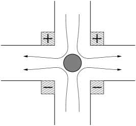
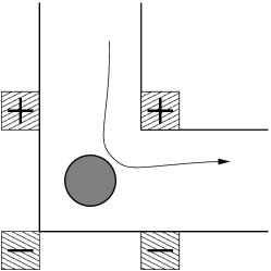
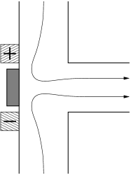
Figure 5: ICEO micropump designs for ‘cross’, ‘elbow’, and ‘T’ junctions. A conducting cylinder placed in a junction of microchannels, subject to an applied AC or DC field, drives an ICEO flow which draws fluid in along the field axis and expels it perpendicular to the field axis. For the four-electrode configurations, the field axis can be switched from vertical to horizontal by switching the polarities of two diagonally opposite electrodes, reversing the pumping direction.

The simplest ICEO-based devices follow natually from the symmetry of ICEO flows, which generally draw fluid in along the field axis and eject it radially. This symmetry can be exploited to drive fluid around a corner where two, three, or four micro-channels converge at right angles, as shown in figure 5. These DC or AC electro-osmotic pumps are reversible: changing the polarity of the four electrodes (shown for the elbow and cross junctions in the figure) so as to change the field direction by 90^∘, reverses the sense of pumping.

For variety, we give an alternate design for the T-junction pump, which uses a conducting plate embedded in the channel wall between the electrodes and cannot be reversed. A reversible T junction, similar to the cross and elbow junctions, could easily be designed. The former design, however, can be modified to reduce the detrimental effects of viscous drag by having the metal plate wrap around to the top and bottom walls (not shown), in addition to the side wall. In general, placing the ‘inducing conductor’ driving ICEO flow on a channel wall is advantageous because it eliminates an inactive surface that would otherwise contribute to viscous drag.

The pressure drop generated by an ICEO junction pump can be estimated on dimensional grounds. The natural pressure scale for ICEO is $P\sim\eta U_{0}/a\sim\varepsilon_{w}E_{0}^{2}$, and the pressure decays with distance like $(a/r)^{2}$. Thus a device driven by a cylinder of radius $a$ in a junction with channel half-width $W$ creates a pressure head of order $\Delta P\sim\varepsilon_{w}E_{0}^{2}a^{2}/W^{2}$. For the specifications listed in Table 2, this corresponds to a pressure head on the order of mPa. This rather small value suggests that straightforward ICEO pumps are better suited for local fluid control than for driving fluids over significant distances.

5.3.2 ICEO micro-mixers

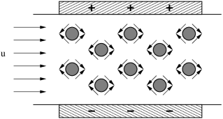
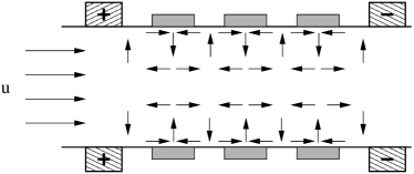
Figure 6: AC electro-osmotic mixers. Diffusive mixing in a background flow is enhanced by the ICEO convection rolls produced by (a) an array of conducting posts in a transverse AC field, and (b) conducting objects (or coatings) embedded in channel walls between micro-electrodes applying fields along the flow direction.

As discussed above, rapid mixing in microfluidic devices is not trivial, since inertial effects are negligible and mixing can only occur by diffusion. Chaotic advection ([Aref (1984)]) provides a promising strategy for mixing in Stokes flows, and various techniques for creating chaotic streamlines have been introduced (e.g. [Liu et al. (2000), Stroock et al. (2002)]). ICEO flows provide a simple method to create micro-vortices, and could therefore be used in a pulsed fashion to create unsteady two-dimensional flows with chaotic trajectories.

In figure 6a, we present a design for an ICEO mixer in which a background flow passes through an array of transverse conducting posts. An AC field in the appropriate frequency range ($\tau_{W}^{-1}\leq\omega\leq\tau_{a}^{-1}$) is applied perpendicular to the posts and to the mean flow direction, which generates an array of persistent ICEO convection rolls. Note that the radius of the posts in the mixer should be smaller than shown ($a\ll W$) to validate the simple approximations made above, where a ‘background’ field is applied to each post in isolation. However, larger posts as shown could have useful consequences, as the final field is amplified by focusing into a smaller region. We leave a careful analysis of such issues for future work.

The same kind of convective mixing could also be produced by a different design, illustrated in figure 6b, in which an AC (or DC) field is applied along the channel with metal stripes embedded in the channel walls. As with the posts described above, the metal stripes are isolated from the electrodes applying the driving field. This design has the advantage that it drives flow immediately adjacent to the wall, which reduces ‘dead space’.

  \begin{picture}(5213.0,2124.0)(2389.0,-3973.0)\end{picture}

Figure 7: Fixed-potential ICEO pumps (left) and mixers (right) can be constructed by electrically coupling the ‘inducing conductor’, which may be a post (as shown) or a surface pattern (not shown), to one set of electrodes. These devices generalize ‘AC electro-osmosis’ in flat-surface electrodes arrays to other situations, with different flow patterns and frequency responses.

5.3.3 Devices exploiting fixed-potential ICEO

By coupling the potential of the posts or plates in the devices above to the electrodes, fixed-potential ICEO can be exploited to generate net pumping past the posts. For example, in the cross-junction pump of figure 5, if the central post were grounded to one of the pairs of electrodes, there would be an enhanced flow sucking fluid in from the channel between the electrode pair (with an AC or DC voltage). Likewise, a fixed-potential ICEO linear pump can be created in the middle of a channel, as shown in figure 7a.

To estimate the flow generated by the single-post device, we note that the post in figure 7a, if freely suspended, would move with velocity $U_{E}\sim\varepsilon_{w}V_{0}^{2}h/\eta L^{2}$ down the channel. The post is held in place, however, which requires a force (per unit length) $F_{\|}\sim 4\pi\eta U_{E}/(\log(W/a)-0.9)$ ([Happel & Brenner (1983)]). The resulting flow rate depends on the length of the channel; however, the pressure required to stop the flow does not. This can be estimated using a two-dimensional analog of the calculation of [Brenner (1958)] for the pressure drop due to a small particle in a cylindrical tube, giving a pressure drop $\Delta P\sim 3F_{\|}/4W$. This pressure drop is larger than that for the fixed-total-charge ICEO junction pumps by a factor of ${\cal O}\left(hW^{3}/a^{2}L^{2}\right)$. Furthermore, multiple fixed-potential ICEO pumps could be placed in series. When the post is small ($a\ll W,L$), these pumps operate in the same frequency range $\tau_{W}^{-1}<\omega<\tau_{c}^{-1},$ as the junction pumps above.

Clearly, many other designs are possible, which could provide detailed flow control for pumping or micro-vortex generation. For example, fixed-potential ICEO can also be used in a micromixer design, as shown in figure 7b, wherein rolls the size of the channel can be established. An interesting point is that frequency response of the ICEO flow is sensitive to both the geometry and the electrical couplings. We leave the design, optimization, and application of real devices for future work, both experimental and theoretical.

We close this section by comparing these new kinds of devices with previous examples of ICEO in microfluidic devices, which involve quasi-planar micro-electrode arrays to produce ‘AC electro-osmosis’ (Ramos et al. 1999; Ajdari 2000). As noted above, when the potential of the ‘inducing conductor’ (post, stripe, etc.) is coupled to the external circuit, it effectively behaves like an electrode, so fixed-potential ICEO is closely related to AC electro-osmosis. Of course, it shares the same fundamental physical mechanism, which we call ‘ICEO’, as do related effects in polarizable colloids that do not involve electrodes. Fixed-potential ICEO devices, however, represent a significant generalization of AC electro-osmotic planar arrays, because a nontrivial distinction arises between ‘electrode’ (applying the field) and ‘inducing conductor’ (producing the primary ICEO flow) in multi-dimensional geometries. This allows a considerable variety of flow patterns and frequency responses. In contrast, existing devices using AC electro-osmosis peak at a single frequency and produce very similar flows (Ramos et al. 1998, 1999; Brown et al. 2001; Studer et al. 2002; Mpholo et al. 2003).

6 Surface contamination by a dielectric coating

The above examples have focused on an idealized situation with a clean metal surface. In this section, we examine the effect of a non-conducting dielectric layer which coats the conductor, and find that any dielectric layer which is thicker than the screening length $\lambda_{D}$ significantly reduces the strength of the ICEO flow. Furthermore, the ICEO flow around a dielectric object, rather than a perfectly conducting object as we have discussed so far, is presented as a limiting case of the analysis in this section.

We start with a simple physical picture to demonstrate the basic effect of a thin dielectric layer. Consider a conducting cylinder of radius $a$ coated with a dielectric layer of thickness $\lambda_{d}\ll a$ (so that the surface looks locally planar) and permeability $\varepsilon_{d}$, as shown in figure 8. In steady state, the potential drop from the conducting surface $\phi=0$ to the potential $\phi_{\infty}$ outside of the double layer occurs across in two steps: across the dielectric (where $E=E_{d}$), and across the screening cloud (where $E=E_{w}$), so that

$$E_{d}\lambda_{d}+E_{w}\lambda_{D}=\phi_{\infty}.$$ (45)

Figure 8: A dielectric layer of thickness $\lambda_{d}$ and permittivity $\varepsilon_{d}$ coating a conductor. The potential drop between the external potential $\phi_{\infty}$ and 0 at the conductor occurs in two steps: $\Delta\phi_{d}=E_{d}\lambda_{d}$ across the dielectric and $\Delta\phi_{w}\approx E_{w}\lambda_{D}$ across the double layer.

The electric fields in the double layer and in the dielectric layer are related via $\varepsilon_{d}E_{d}=\varepsilon_{w}E_{w}$, so that

$$\left(1+\frac{\varepsilon_{w}}{\varepsilon_{d}}\frac{\lambda_{d}}{\lambda_{D}}\right)E_{w}\lambda_{D}=\phi_{\infty}.$$ (46)

Since $E_{w}\lambda_{D}$ is approximately the potential drop $\zeta$ across the double-layer, and since the steady-state bulk potential is given by (14) to be $\phi_{\infty}=2E_{0}a\cos\theta$, we find the induced-charge zeta potential to be

$$\zeta=\frac{2E_{0}a\cos\theta}{1+\varepsilon_{w}\lambda_{d}/\varepsilon_{d}\lambda_{D}}.$$ (47)

Thus unless the layer thickness $\lambda_{d}$ is much less than $\varepsilon_{d}\lambda_{D}/\varepsilon_{w}$, the bulk of the potential drop $\phi_{\infty}$ occurs across the dielectric layer, instead of the double-layer, resulting in a reduced electro-osmotic slip velocity.

The modification to the charging time $\tau_{c}$ for the coated cylinder can likewise be understood from this picture. The dielectric layer represents an additional (parallel-plate) capacitor of separation $\lambda_{d}$ and filled with a dielectric $\varepsilon_{d}$, in series with the capacitive screening cloud, giving a total capacitance

$$C_{T}=\frac{\varepsilon_{w}}{\lambda_{D}}\left(1+\frac{\varepsilon_{w}\lambda_{d}}{\varepsilon_{d}\lambda_{D}}\right)^{-1},$$ (48)

and a modified RC time

$$\tau_{c}=\frac{\lambda_{D}a}{D}\left(1+\frac{\varepsilon_{w}\lambda_{d}}{\varepsilon_{d}\lambda_{D}}\right)^{-1},$$ (49)

as found by [Ajdari (2000)] for a similar calculation for a compact (Stern) layer. A discussion of double-layer capacitance in the nonlinear regime, where the compact layer is approximated by a thin dielectric layer is given by [Macdonald (1954)].

A full calculation of the induced zeta potential around a dielectric cylinder of radius $a$ coated by another dielectric layer with outer radius $b$ and thickness $(b-a)$ is straightforward although cumbersome. (Note that the analogous problem for a coated conducting sphere was treated by [A. S. Dukhin (1986)] as a model of a dead biological cell.) The resulting induced-charge zeta potential is

$$\zeta=\frac{2bE_{0}(1+\Gamma_{c})\cos\theta}{2+\kappa b(1-\Gamma_{c})},$$ (50)

with characteristic charging time scale

$$\tau_{c}=\frac{\lambda_{D}b}{D}\left[1+\frac{\kappa b}{2}(1-\Gamma_{c})\right]^{-1},$$ (51)

where $\Gamma_{c}$ is defined to be

$$\Gamma_{c}=\frac{b^{2}+a^{2}-\varepsilon_{w}/\varepsilon_{d}(b^{2}-a^{2})}{b^{2}+a^{2}+\varepsilon_{w}/\varepsilon_{d}(b^{2}-a^{2})}.$$ (52)

It is instructive to examine limiting cases of the induced zeta potential (50). In the limit of a ‘conducting’ dielectric coating $\varepsilon_{d}/\varepsilon_{w}\rightarrow\infty$, we recover the standard result for ICEO around a metal cylinder, as expected. In the limit of a thin dielectric layer $b=a+\lambda_{d}$, where $\lambda_{d}\ll a$, the induced zeta potential is given by

$$\zeta(\lambda_{d}\ll a)\approx\frac{2bE_{0}\cos\theta}{1+\lambda_{d}\varepsilon_{w}/\lambda_{D}\varepsilon_{d}},$$ (53)

as found in (47), with a charging time

$$\tau_{c}(\lambda_{d}\ll a)\approx\frac{\lambda_{D}b}{D}\left(1+\frac{\varepsilon_{w}\lambda_{d}}{\varepsilon_{d}\lambda_{D}}\right)^{-1},$$ (54)

as found in (49). Therefore, the ICEO slip velocity around a coated cylinder is close to that of a clean conducting cylinder ($\zeta=2bE_{0}\cos\theta$) only when the dielectric layer is much thinner than the screening length times the dielectric contrast, $\lambda_{d}\ll\lambda_{D}\varepsilon_{d}/\varepsilon_{w}$. The zeta potential induced around a conducting cylinder with a thicker dielectric layer,

$$\zeta(\lambda_{d}\gg\lambda_{D})\approx 2bE_{0}\frac{\varepsilon_{d}\lambda_{D}}{\varepsilon_{w}\lambda_{d}}\cos\theta,$$ (55)

is smaller by a factor of ${\cal O}\left(\lambda_{D}/\lambda_{d}\right)$, and the charging time,

$$\tau_{c}(\lambda_{d}\gg\lambda_{D})\approx\frac{\varepsilon_{w}\lambda_{D}}{\varepsilon_{d}\lambda_{d}}\frac{\lambda_{D}b}{D},$$ (56)

is likewise shorter by a factor of ${\cal O}\left(\lambda_{D}/\lambda_{d}\right)$. As a result, strong ICEO flow requires a rather clean and highly polarizable surface, with minimal non-conducting deposits.

Note that the limit of a pure dielectric cylinder of radius $b$ is found by taking the limit $a\rightarrow 0$. This gives a zeta potential of

$$\zeta(a=0)\rightarrow\frac{2bE_{0}\cos\theta}{1+\varepsilon_{w}b/\varepsilon_{d}\lambda_{D}}\approx 2\frac{\varepsilon_{d}}{\varepsilon_{w}}E_{0}\lambda_{D}\cos\theta,$$ (57)

and an ICEO slip velocity which is smaller than the conducting case (17) by ${\cal O}\left(\lambda_{D}/b\right)$. The charging time for a dielectric cylinder is given by

$$\tau_{c}(a=0)\approx\frac{\varepsilon_{w}}{\varepsilon_{d}}\frac{\lambda_{D}^{2}}{D},$$ (58)

as expected from (49) in the limit $\lambda_{d}\gg\lambda_{D}$.

7 Induced-charge electro-osmosis: systematic derivation

In this section, we provide a systematic derivation of induced-charge electro-osmosis, in order to complement the physical arguments above. We derive a set of effective equations for the time-dependent ICEO flow around an arbitrarily-shaped conducting object, and indicate the conditions under which the approximations made in this article are valid. Starting with the usual ‘electrokinetic equations’ for the electrostatic, fluid, and ion fields (as given by, e.g. , [Hunter (2000)]), we propose an asymptotic expansion that matches an inner solution (valid within the charge cloud) with an outer region (outside of the charge cloud), and that accounts for two separate time scales–the time for the charge cloud to locally equilibrate and the time scale over which the external electric field changes.

Although it has mainly been applied to steady-state problems, the method of matched asymptotic expansions is well established in this setting, where it is commonly called the ‘thin double layer approximation’. For simplicity, like many authors, we perform our analysis for the case of a symmetric binary electrolyte with a single ionic diffusivity in a weak applied field, and we compute only the leading-order uniformly valid approximation. The same simplifying assumptions were also made by [Gonzalez et al. (2000)] in their recent asymptotic analysis of AC electro-osmosis.

In the phenomenological theory of diffuse charge in dilute electrochemical systems, the electrostatic field obeys Poisson’s equation,

$$\nabla^{2}\phi=-\frac{(n_{+}-n_{-})e}{\varepsilon_{w}},$$ (59)

where $n_{\pm}$ represent the local number densities of positive and negative ions. These obey conservation equations

$$\frac{\partial n_{\pm}}{\partial t}+\nabla\cdot(n_{\pm}{\bf v}_{\pm})=0,$$ (60)

where ${\bf v}_{\pm}$ represent the velocities of the two ion species,

$${\bf v}_{\pm}=\mp be\nabla\phi-k_{B}Tb\nabla\log n_{\pm}+{\bf u},$$ (61)

where $b$ is the mobility of the ions in the solvent and ${\bf u}$ is the local fluid velocity. Terms in (61) represent ion motion due to (a) electrostatic forcing, (b) diffusion down density gradients, and (c) advection with the local fluid velocity. The fluid flow obeys the Stokes equations, with body force given by the product of the charge density with the electric field,

$$\eta\nabla^{2}{\bf u}-\nabla p=e(n_{+}-n_{-})\nabla\phi,$$ (62)

along with incompressibility. Strictly speaking, this form does not explicitly include osmotic pressure gradients, as detailed below. However, osmotic forces can be absorbed into a modified pressure field $p$, and the resulting flow is unaffected.

For boundary conditions on the surface $\Gamma$ of the conductor, we require the fluid flow to obey the no-slip condition, the electric potential to be an equipotential (with equilibrium zeta potential $\zeta_{0}$), and the ions to obey a no-flux condition:

$${\bf u}(\Gamma) = {\bf 0}$$ (63)

$$\phi(\Gamma) = \zeta_{0}$$ (64)

$${\bf\hat{n}}\cdot{\bf v}_{\pm}(\Gamma) = 0,$$ (65)

where ${\bf\hat{n}}$ represents the (outer) normal to the surface $\Gamma$. Far from the object, we require the fluid flow to decay to zero, the electric field to approach the externally-applied electric field, and the ion densities $n_{\pm}$ to approach their constant (bulk) value $n_{0}$.

In order to simplify these equations, we insert (61) in (60), and take the sum and difference of the resulting equations for the two ion species to obtain

$$\dot{c}^{\rho}+D\kappa^{2}c^{\rho}-D\nabla^{2}c^{\rho}-eb\nabla\cdot\left[c^{e}\nabla\phi\right]+{\bf u}\cdot\nabla c^{\rho} = 0$$ (66)

$$\dot{c}^{e}-D\nabla^{2}c^{e}-eb\nabla\cdot\left[c^{\rho}\nabla\phi\right]+{\bf u}\cdot\nabla c^{e} = 0,$$ (67)

where we have used (59) and where we have defined

$$c^{e} = n_{+}+n_{-}-2n_{0}$$ (68)

$$c^{\rho} = n_{+}-n_{-}.$$ (69)

The first variable, $c^{e}$, represents the excess total concentration of ions, while the second, $c^{\rho}$, is related to the charge density via $c^{\rho}=\rho/e$. The first three terms in (66) represent a (possible) transient, electrostatic transport, and diffusive transport, respectively, and will be seen to give the dominant balance in the double layer. The next term represents the divergence of a flux of excess ionic concentration $c^{e}$ (but not excess charge) due to an electric field. The final term represents ion advection with the fluid flow ${\bf u}$. The analogous (67) for the charge-neutral $c^{e}$ lacks the electrostatic transport term. Both $c^{e}$ and $c^{\rho}$ decay away from the solid surface and obey the no-flux boundary conditions (65),

$${\bf{\hat{n}}}\cdot\nabla c^{\rho}|_{\Gamma} = -\frac{e}{k_{B}T}(2n_{0}+c^{e}){\bf{\hat{n}}}\cdot\nabla\phi|_{\Gamma}$$ (70)

$${\bf{\hat{n}}}\cdot\nabla c^{e}|_{\Gamma} = -\frac{e}{k_{B}T}c^{\rho}{\bf{\hat{n}}}\cdot\nabla\phi|_{\Gamma},$$ (71)

at the surface $\Gamma$.

In what follows, we obtain an approximate solution to the governing equations (59), (66), and (67), at the leading order in a matched asymptotic expansion. We first analyze the solution in the ‘inner’ region within a distance of order $\lambda_{D}$ of the surface. Non-dimensionalization yields a set of approximate equations for the inner region and a set of matching boundary conditions which depend on the ‘outer’ solution, valid in the quasi-neutral bulk region (farther than $\lambda_{D}$ from the surface). Similarly, approximate equations and effective boundary conditions for the outer region are found. By solving the inner problem and matching to the outer problem, a set of effective equations are derived for time-dependent, bulk ICEO flows.

7.1 Non-dimensionalization and ‘inner’ region

We begin by examining the ‘inner region’, adjacent to the conducting surface. Denoting non-dimensional variables in the inner region with tildes, we scale variables as follows,

$${\bf r}=\lambda_{D}\tilde{{\bf r}},\ \ t=(\kappa^{2}D)^{-1}\tilde{t},\ \ \phi=\Phi_{0}\tilde{\phi},\ \ {\bf u}=U_{0}\tilde{{\bf u}},\ c^{\rho}=2n_{0}\Psi\tilde{c}^{\rho},\ c^{e}=2n_{0}\Psi^{2}\tilde{c}^{e},\ \ {\bf E}=E_{0}\tilde{{\bf E}}$$ (72)

where $\Phi_{0}$ and $U_{0}$ are potential and velocity scales (left unspecified for now), and where we have introduced the dimensionless surface potential,

$$\Psi=\frac{e\Phi_{0}}{k_{B}T}.$$ (73)

Note that $\tilde{c}^{e}$ scales with $\Psi^{2}$ to satisfy the dominant balance in (67). Finally, we have scaled time with the Debye time, $\tau_{D}=(\kappa^{2}D)^{-1}=\lambda_{D}^{2}/D$, although the analysis will dictate another time scale, as expected from the physical arguments above.

The dimensionless ion conservation equations (66-67) become

$$\frac{\partial\tilde{c}^{\rho}}{\partial\tilde{t}}+\tilde{c}^{\rho}-\tilde{\nabla}^{2}\tilde{c}^{\rho}-\Psi^{2}\tilde{\nabla}\cdot\left[\tilde{c}^{e}\tilde{\nabla}\tilde{\phi}\right]-{\rm Pe}\,\tilde{{\bf u}}\cdot\tilde{\nabla}\tilde{c}^{\rho} = 0$$ (74)

$$\frac{\partial\tilde{c}^{e}}{\partial\tilde{t}}+\tilde{\nabla}^{2}\tilde{c}^{e}+\tilde{\nabla}\cdot\left[\tilde{c}^{\rho}\tilde{\nabla}\tilde{\phi}\right]-{\rm Pe}\,\tilde{{\bf u}}\cdot\tilde{\nabla}\tilde{c}^{e} = 0,$$ (75)

where we have introduced the Péclet number,

$$\mbox{Pe}=\frac{U_{0}}{\kappa D}.$$ (76)

The boundary conditions (70-71) in non-dimensional form are given by

$${\bf{\hat{n}}}\cdot\tilde{\nabla}\tilde{c}^{\rho}|_{\Gamma} = -(1+\Psi^{2}\tilde{c}^{e}){\bf{\hat{n}}}\cdot\tilde{\nabla}\tilde{\phi}|_{\Gamma}$$ (77)

$${\bf{\hat{n}}}\cdot\tilde{\nabla}\tilde{c}^{e}|_{\Gamma} = -\tilde{c}^{\rho}{\bf{\hat{n}}}\cdot\tilde{\nabla}\tilde{\phi}|_{\Gamma}.$$ (78)

In the analysis that follows, we concentrate on the simplest limiting case. We assume the screening length to be much smaller than any length $L_{0}$ associated with the surface geometry, parametrized through

$$\epsilon=(\kappa L_{0})^{-1}=\lambda_{D}/L_{0}\ll 1,$$ (79)

so that the screening cloud ‘looks’ locally planar. As mentioned above, the singular limit of thin double layers, $\epsilon\ll 1$, is the usual basis for the matched asymptotic expansion. The regular limit of small Péclet number, $\mbox{Pe}\ll 1$, which holds in almost any situation, is easily taken by setting $\mbox{Pe}=0$. Finally, we consider the regular limit of small (dimensionless) surface potential, $\Psi\ll 1$, which is the same limit that allows the Poisson-Boltzmann equation to be linearized. With these approximations, the system is significantly simplified: First, $\tilde{c}^{\rho}$ is coupled to $\tilde{c}^{e}$ only through terms of order ${\cal O}\left(\Psi^{2}\right)$ in (74) and boundary condition (77). Second, $\tilde{c}^{e}$ is smaller than $\tilde{c}^{\rho}$ by a factor $\Psi$, and is thus neglected: $\tilde{c}^{\rho}=0+{\cal O}\left(\Psi^{2}\right)$.

In this limit, we obtain the linear Debye equation and boundary condition for $\tilde{c}^{\rho}$ alone:

$$\frac{\partial\tilde{c}^{\rho}}{\partial\tilde{t}}+\tilde{c}^{\rho}=\epsilon^{2}\tilde{\nabla}^{2}\tilde{c}^{\rho}$$ (80)

$${\bf{\hat{n}}}\cdot\tilde{\nabla}\tilde{c}^{\rho}|_{\Gamma}=-{\bf{\hat{n}}}\cdot\tilde{\nabla}\tilde{\phi}|_{\Gamma}.$$ (81)

The potential is then recovered from (59) in the form,

$$\tilde{\nabla}^{2}\tilde{\phi}=-\tilde{c}^{\rho},$$ (82)

with the far-field boundary condition,

$$\tilde{\nabla}\tilde{\phi}\rightarrow-\frac{E_{0}L}{\Phi_{0}}\tilde{{\bf E}},$$ (83)

and the (equipotential) surface boundary condition

$$\tilde{\phi}(\Gamma)=\Phi_{0}\tilde{\zeta}_{0}.$$ (84)

where $\tilde{\zeta}_{0}$ is the dimensionless equilibrium zeta potential.

Since $\epsilon\ll 1$, we introduce a locally Cartesian coordinate system $\{\tilde{n},\tilde{l}\}$, where $\tilde{n}$ is locally normal to the surface, and $\tilde{l}$ is locally tangent to the surface. The governing equations (80) and (82) are both linear in $\tilde{c}^{\rho}$ and $\tilde{\phi}$, which allows the electrostatic and ion fields to be expressed as a simple superposition of the equilibrium fields,

$$\tilde{c}^{\rho}_{\rm eq}=-\tilde{\phi}_{\rm eq}=\tilde{\zeta}_{0}e^{-\tilde{n}},$$ (85)

and the time-dependent induced fields $\tilde{c}^{\rho}_{\rm i}$ and $\tilde{\phi}_{\rm i}$, via

$$\tilde{c}^{\rho}=\tilde{c}^{\rho}_{\rm eq}+\tilde{c}^{\rho}_{\rm i}$$ (86)

$$\tilde{\phi}=\tilde{\phi}_{\rm eq}+\tilde{\phi}_{\rm i}.$$ (87)

The induced electrostatic and ion fields must then obey

$$\tilde{\nabla}^{2}\tilde{\phi}_{i}=-\tilde{c}^{\rho}_{i}$$ (88)

$$\frac{\partial\tilde{c}^{\rho}_{i}}{\partial\tilde{t}}+\tilde{c}^{\rho}_{i}-\tilde{\nabla}^{2}\tilde{c}^{\rho}_{i}=0,$$ (89)

subject to boundary conditions

$$\tilde{\phi}_{i}(\Gamma) = 0$$ (90)

$${\bf{\hat{n}}}\cdot\tilde{\nabla}\tilde{c}^{\rho}_{i}|_{\Gamma} = -{\bf{\hat{n}}}\cdot\tilde{\nabla}\tilde{\phi}_{i}|_{\Gamma},$$ (91)

on the surface.

Another consequence of the linearity of (80) and (82), and therefore of the decoupling of the equilibrium and induced fields, is that different characteristic scales can be taken for the two sets of fields. We scale the potential in the equilibrium problem with the equilibrium zeta potential $\zeta_{0}$, and the potential in the induced problem with $E_{0}L_{0}$, the potential drop across the length scale of the object. In order that the total surface potential be small $(\Psi\ll 1)$, however, we require that the total zeta potential be small,

$$\frac{(|\zeta_{0}|+|E_{0}L_{0}|)e}{k_{B}T}\ll 1.$$ (92)

At the end of this section, we will briefly discuss the rich variety of nonlinear effects which generally occur, in addition to ICEO, when this condition is violated.

We expect the charge cloud $\tilde{c}^{\rho}$ and electric potential $\tilde{\phi}$ to vary quickly with $\tilde{n}$, but slowly with $\tilde{l}$ (along the surface). Furthermore, we expect the charge cloud to exhibit two time scales: a fast (transient) time scale, over which $\tilde{c}^{\rho}$ reaches a quasi-steady dominant balance, and a slow time scale $\tilde{\tau_{c}}$, over which the quasi-steady solution changes. The physical arguments leading to (28) for the charging time suggest that this slow time scale is given by $\tilde{\tau}_{c}=1/\epsilon$, which is not obvious a priori, but which will be confirmed by the successful asymptotic matching.

In order to focus on the long-time dynamics of the induced charge cloud, and guided by the above expectations, we attempt a quasi-steady solution to (88) – (91) of the form

$$\tilde{c}^{\rho}_{i}=\tilde{c}^{\rho}_{i}(\tilde{n},\epsilon\tilde{l},\epsilon\tilde{t})$$ (93)

$$\tilde{\phi}_{i}=\tilde{\phi}_{i}(\tilde{n},\epsilon\tilde{l},\epsilon\tilde{t}).$$ (94)

It can be verified that

$$\tilde{c}^{\rho}_{i} = A(\epsilon\tilde{l},\epsilon\tilde{t})e^{-\tilde{n}}-\epsilon\frac{\dot{A}(\epsilon\tilde{l},\epsilon\tilde{t})}{2}\tilde{n}e^{-\tilde{n}}$$ (95)

$$\tilde{\phi}_{i} = -A(\epsilon\tilde{l},\epsilon\tilde{t})e^{-\tilde{n}}+\epsilon\frac{\dot{A}(\epsilon\tilde{l},\epsilon\tilde{t})}{2}\left[2e^{-\tilde{n}}+\tilde{n}e^{-\tilde{n}}\right]+B(\epsilon\tilde{l},\epsilon\tilde{t})+C(\epsilon\tilde{l},\epsilon\tilde{t})\tilde{n},$$ (96)

solve the governing equations to ${\cal O}\left(\epsilon^{2}\right)$.

The equipotential boundary condition (90) is satisfied when

$$A(\epsilon\tilde{l},\epsilon\tilde{t})=B(\epsilon\tilde{l},\epsilon\tilde{t})+\epsilon\dot{A}(\epsilon\tilde{l},\epsilon\tilde{t}),$$ (97)

so that the induced double-layer charge density is proportional (to leading order in $\epsilon$) to the potential just outside the double layer. The normal ion flux condition (91),

$$\epsilon\dot{A}(\epsilon\tilde{l},\epsilon\tilde{t})=C(\epsilon\tilde{l},\epsilon\tilde{t}),$$ (98)

relates the evolution of the double-layer charge density to the electric field normal to the double-layer. Matching the inner region to the outer region provides the final relations. In the limit $\tilde{n}\rightarrow\infty$, the electrostatic and ion fields approach their limiting behavior

$$\tilde{c}^{\rho} \rightarrow 0$$ (99)

$$\tilde{\phi} \rightarrow B(\epsilon\tilde{l},\epsilon\tilde{t})+C(\epsilon\tilde{l},\epsilon\tilde{t})\tilde{n}.$$ (100)

7.2 Outer solution

We now turn to the region outside of the double-layer, and use overbars to denote ‘outer’ non-dimensional variables (scaled with length scale $L_{0}$ and potential scale $E_{0}L_{0}$). According to (95) and (99), any non-zero charge density $\bar{c}^{\rho}$ that exists within the inner region decays exponentially away from the surface $\Gamma$. A homogeneous solution ($\bar{c}^{\rho}_{o}=0$) thus satisfies (80) and the decaying boundary condition at infinity. With $\bar{c}^{\rho}_{o}=0$, (82) for the electrostatic field $\bar{\phi}_{o}$ in the outer region reduces to Laplace’s equation,

$$\bar{\nabla}^{2}\bar{\phi}_{o}=0,$$ (101)

with far-field boundary condition (83) given by

$$\bar{\nabla}\bar{\phi}_{o}\rightarrow-\hat{{\bf E}}.$$ (102)

To determine $\bar{\phi}_{o}$ uniquely, one further boundary condition on the surface $\Gamma$ is required, which is obtained by matching to the inner solution. The limiting value of the ‘outer’ field $\bar{\phi}_{o}$,

$$\bar{\phi}_{o}(\bar{{\bf r}}\rightarrow\Gamma)\rightarrow\bar{\phi}_{0}(\Gamma)+\hat{E}_{\perp}(\Gamma)\bar{n},$$ (103)

must match the inner solution (100), which gives two relations

$$B(\epsilon\tilde{l},\epsilon\tilde{t})=\tilde{\phi}_{0}(\tilde{l}),$$ (104)

$$C(\epsilon\tilde{l},\epsilon\tilde{t})=\epsilon\tilde{E}_{\perp}(\tilde{l}).$$ (105)

Using (105) in (98), the fact that $C$ is ${\cal O}\left(\epsilon\right)$ verifies that the assumed time scale $\tau_{c}=\tau_{D}/\epsilon$ for induced double layer evolution is indeed correct, as expected from physical arguments (28).

7.3 Effective equations for ICEO in weak applied fields

Using the above results, we present a set of effective equations for time-dependent ICEO that allows the study of the large-scale flows, without requiring the detained inner solution. What emerges is a first-order ODE for the dimensionless total surface charge density in the diffuse double layer, $\tilde{q}=A$, so an ‘initial’ value for $\tilde{q}$ must be specified. From (97) and (104), the ‘outer’ potential on the surface $\Gamma$ is given by

$$\bar{\phi}_{o}(\Gamma,\epsilon\bar{t})=\tilde{q}(\Gamma,\epsilon\bar{t}),$$ (106)

which, along with the far-field boundary condition (83), uniquely specifies the solution to Laplace’s equation (101). From this solution, the normal field $\hat{E}_{\perp}(\Gamma,\epsilon\bar{t})$ is found, which (using (105) and (98)) results in a time-dependent boundary condition,

$$\frac{\partial\tilde{q}}{\partial\bar{t}}=\epsilon\hat{E}_{\perp}(\Gamma,\epsilon\bar{t}),$$ (107)

which is more naturally expressed as

$$\frac{\partial\tilde{q}}{\partial\hat{t}}=\hat{E}_{\perp}(\Gamma,\hat{t}),$$ (108)

in terms of the dimensionless time variable, $\hat{t}=\epsilon\bar{t}=t/\tau_{c}$.

We have thus matched the bulk field outside the charge cloud with the ‘inner’ behavior of the charge cloud in a self-consistent manner. The ‘inner’ solutions for $c^{\rho}$ and $\zeta$ equilibrate quickly in response to the (slow) charging, and affect the boundary conditions which determine the ‘outer’ solution. Matching (105) and (98) results in a relation between the charge cloud and normal ionic flux, confirming the validity of (13) and (25), which were previously argued in an intuitive, physical manner. This analysis has demonstrated that errors to this approach are of order ${\cal O}\left(\Psi^{2}\right)$, ${\cal O}\left(P\right)$ and ${\cal O}\left(\epsilon^{2}\right)$. In this limit, the system evolves with a single characteristic time scale, $\tau_{c}=\lambda_{D}L_{0}/D$, set by asymptotic matching, which physically corresponds to an RC coupling, as explained above.

7.4 Fluid dynamics

7.4.1 Fluid body forces: electrostatic and osmotic

Thus far, we have derived the effective equations for the dynamics of the induced double-layer. To conclude, we examine the ICEO slip velocity that results from the interaction of the applied field and the induced diffuse layer. We demonstrate that, in the limits of thin double layer and small surface potential, the Smoluchowski formula (4) for fluid slip holds.

Following [Levich (1962)] (p. 484), we consider a conducting surface $\Gamma$ immersed in a fluid, with an applied ‘background’ electrostatic potential $\phi_{o}$. In addition, a thin double-layer (with potential $\xi$) exists and obeys

$$\nabla^{2}\xi=-\frac{(n_{+}-n_{-})e}{\varepsilon_{w}}=-\frac{n_{0}e}{\varepsilon_{w}}\left(e^{-e\xi/k_{B}T}-e^{e\xi/k_{B}T}\right),$$ (109)

so that the total potential $\phi=\phi_{o}+\xi$. Note that this assumes that the double layer is in quasi-equilibrium.

Fluid stresses have two sources: electric and osmotic. The electric stress in the fluid is given by the Maxwell Stress tensor,

$$T_{ij}=\varepsilon_{w}\left(E_{i}E_{j}-\frac{1}{2}{\bf E}\cdot{\bf E}\delta_{ij}\right),$$ (110)

from which straightforward manipulations yield the electrical body force on the fluid to be

$${\bf F}_{E}\equiv\nabla\cdot{\bf T}=\varepsilon_{w}\nabla\phi\nabla^{2}\phi\equiv\varepsilon_{w}\nabla(\phi_{o}+\xi)\nabla^{2}\xi.$$ (111)

Osmotic stresses come from gradients in ion concentration, and exert a fluid body force

$${\bf F}_{O}=-k_{B}T\nabla\left(n_{+}+n_{-}\right)=e\nabla\zeta\left(n_{+}-n_{-}\right)=-\varepsilon_{w}\nabla\xi\nabla^{2}\xi.$$ (112)

Thus the total body force on the fluid, is given by the sum of ${\bf F}_{E}$ and ${\bf F}_{O}$,

$${\bf F}=\varepsilon_{w}\nabla\phi_{o}\nabla^{2}\xi=\rho{\bf E}_{B}.$$ (113)

Therefore, when both electric and osmotic stresses are included, the body force on the double layer above a conductor is given by the product of the local charge density $\rho$ and the ‘background’ electric field ${\bf E}_{B}=-\nabla\phi_{o}$ (which, importantly, does not vary across the double layer). Note also that the same fluid flow would result if the double-layer forcing $\rho({\bf E}_{B}+{\bf E}_{\xi})$ were to be used, since the osmotic component (112) is irrotational and can be absorbed in a modified fluid pressure.

7.4.2 ICEO slip velocity

Finally, we examine the ICEO slip velocity that results when the electric field $-\nabla\phi_{o}$ drives the ions in the induced charge screening cloud $\rho$.

We look first at the flow in the ‘inner’ region of size $\lambda_{D}$. For the ICEO slip velocity to reach steady state, vorticity must diffuse across the double layer, which requires a very small time $\tau_{\omega}(\lambda_{D})=\lambda_{D}^{2}/\nu\approx 10^{-10}$ s. Because $\tau_{\omega}$ is so much faster than the charging time and Debye time, we consider the ICEO slip velocity to follow changes in $\zeta$ or $\phi$ instantaneously. As noted above, the unsteady term may play a role in cutting off the oscillating component of the bulk flow. However, our main concern is with the steady, time-averaged component, which simply obeys the steady, forced Stokes equation.

Non-dimensionalizing as above, we re-express the forced Stokes equations (62), with forcing given by (113), using a stream function $\psi$ defined so that $u_{l}=\partial_{n}\psi$ and $u_{n}=-\partial_{l}\psi$. The stream function obeys

$$\tilde{\nabla}^{4}\tilde{\psi}=\left(\frac{\partial\tilde{c}^{\rho}}{\partial\tilde{n}}\frac{\partial\tilde{\phi}}{\partial\tilde{l}}-\frac{\partial\tilde{c}^{\rho}}{\partial\tilde{l}}\frac{\partial\tilde{\phi}}{\partial\tilde{n}}\right),$$ (114)

where the stream function has been scaled by $\psi=(\varepsilon_{w}E_{0}\zeta_{0}/\eta\kappa)\tilde{\psi}.$ We perform a local analysis around the point $\tilde{l}=0$ of the ICEO flow driven by an applied tangential electric field $\{\tilde{E}_{\|},\tilde{E}_{\perp}\}$. Using representations of $\tilde{c}^{\rho}$ and $\tilde{\phi}$ around $\tilde{l}=0$,

$$\tilde{c}^{\rho} = \tilde{c}^{\rho}(\epsilon\tilde{l})e^{-\tilde{n}}$$ (115)

$$\tilde{\phi} = -\tilde{E}_{\|}\tilde{l}(\epsilon\tilde{l},\epsilon\tilde{n})-\tilde{E}_{\perp}\tilde{n}(\epsilon\tilde{l},\epsilon\tilde{n}),$$ (116)

it is straightforward to solve (114) to ${\cal O}\left(\epsilon\right)$. The tangential and normal flows are then given by

$$u_{l} = -\frac{\varepsilon_{w}}{\mu}\left[\left(\zeta(l)E_{\|}(l)+\epsilon\frac{\partial\zeta}{\partial\tilde{l}}E_{\perp}\right)\left(1-e^{-\kappa n}\right)+\epsilon\frac{\partial E_{\|}}{\partial\tilde{n}}\left(3-(3+\kappa n)e^{-\kappa n}\right)\right]$$ (117)

$$u_{n} = -\epsilon\frac{\varepsilon_{w}}{\mu}\frac{\partial}{\partial\tilde{l}}\left(\zeta E_{\|}\right)\left(1-\kappa n-e^{-\kappa n}\right),$$ (118)

where $\zeta(l)E_{\|}$ contains terms of ${\cal O}\left(\epsilon\right)$. To leading order, then, the slip flows obey

$$u_{l}\rightarrow-\frac{\varepsilon_{w}}{\mu}\zeta(l)E_{\|}(l)+{\cal O}\left(\epsilon\right)\ \ \mbox{and}\ \ u_{n}={\cal O}\left(\epsilon\right).$$ (119)

The tangential flow does indeed asymptote to (4), with local zeta potentials and background field, and the normal flow velocity is smaller by a factor of order ${\cal O}\left(\epsilon\right)$.

Thus an ICEO slip velocity is very rapidly established in response to an induced zeta potential and ‘outer’ tangential field. Furthermore, despite double-layer and tangential field gradients, the classical Helmholtz-Smoluchowski formula, (4), correctly gives the electro-osmotic slip velocity. This may seem surprising, given that the tangential field vanishes at the conducting surface.

The final step involves finding the bulk ICEO flow must be found by solving the unsteady Stokes equations, with no forcing, but with a specified ICEO slip velocity on the boundary $\Gamma$, given by solving the effective electrokinetic transport problem above.

7.5 Other nonlinear phenomena at large voltages

Although we have performed our analysis in the linearized limit of small potentials, it can be generalized to the ‘weakly nonlinear’ limit of thin double layers, where (7) holds and $\mbox{Du}\ll 1$. In that case, the bulk concentration remains uniform at leading order, and the Helmholtz-Smoluchowski slip formula remains valid. The main difference involves the time-dependence of double-layer relaxation, which is slowed down by nonlinear screening once the thermal voltage is exceeded. It can be shown that the linear time-dependent boundary condition, (13) or (108), must be modified to take into account the nonlinear differential capacitance, as in (34). Faradaic surface reactions and the capacitance of the compact Stern layer may also be included in such an approach, as in the recent work of [Bonnefont et al. (2001)].

The condition (7) for the breakdown of Smoluchowski’s theory of electrophoresis (with $\zeta=\zeta_{0}+E_{0}a$) coincides with the condition $\tau_{c}(\zeta)\ll\tau_{D}$, where $\tau_{c}$ takes into account the nonlinear differential capacitance (36). When this condition is violated (the ‘strongly nonlinear’ regime), double-layer charging is slowed down so much by nonlinearity that it continues to occur at the time scale of bulk diffusion. At such large voltages, the initial charging process draws so much neutral concentration into the double layer that it creates a transient diffusion layer which must relax into the bulk, while coupled to the ongoing double-layer charging process. [Bazant, Thornton & Ajdari (2004)] explore such processes.

In the strongly nonlinear regime, the Dukhin number is typically not negligible, and bulk concentration gradients (and their associated electrokinetic effects) are produced by surface conduction (see [S. S. Dukhin (1993)] and [Lyklema (1991)]). Tangential concentration gradients modify the usual electro-osmotic slip by changing the bulk electric field (concentration polarization) and by producing diffusio-osmotic slip. Therefore, both the steady state and the relaxation processes for ICEO flows are affected.

Finally, large voltages can also lead to the breakdown of ideal polarizability via spontaneous Faradaic reactions on different sides of the object, as noted by [Murtsovkin (1991)]. [Gamayunov et al. (1992)] observed that the induced-charge electro-osmotic flow around metal colloidal spheres reverses direction for large colloids, and argued that Faradaic reactions were responsible. Furthermore, [Barany et al. (1998)] measured large conducting colloids to have ‘superfast’ (second-kind) electrophoretic velocities. They argued that sufficiently strong fields cause Faradaic currents at the two sides of the colloid (as though they were electrodes), resulting in the development of a bulk ‘space charge’ and, correspondingly, second-kind electrophoresis.

A complete description of time-dependent ICEO at large voltages, which is beyond the scope of this article, would require considering all of these effects at once. The approximation of thin double layers, which has been applied mostly to steady-state problems involving non-polarizable objects, is a good starting point. However, the presence of multiple length and time scales complicates mathematical analysis, especially in any attempt to go beyond the leading-order approximation. An important goal, therefore, would be to extend the method of matched asymptotic expansions to derive effective equations and boundary conditions for strongly nonlinear ICEO and to carefully analyze asymptotic corrections.

8 Summary and Discussion

In this article, we have described the general phenomenon of induced-charge electro-osmosis (ICEO), which includes a wide variety of techniques (both old and new) for driving steady micro-flows around conducting or dielectric surfaces using AC or DC electric fields. We have given a physical picture of the basic mechanism for ICEO, involving the inhomogeneous surface charge induced in the conductor in order to maintain an equipotential surface in the presence of an applied field. In response, the electric field normal to the surface/charge cloud drives ions into an inhomogeneous (dipolar) charge cloud, which are in turn driven by the tangential electric field. This results in ICEO slip velocities of magnitude $U_{0}\sim\varepsilon_{w}E_{0}^{2}a/\eta$. A charging time scale $\tau_{c}\sim\lambda_{D}a/D$ is required for these induced charge clouds to form. Due to the dependence on the square of the applied field $E_{0}$, a nonzero time-averaged ICEO flow can be driven using AC fields of sufficiently low frequencies $(\omega\ll 1/\tau_{c})$.

We have performed explicit calculations for the steady and unsteady ICEO slip velocities (suddenly-applied and sinusoidal fields) around symmetric conducting cylinders. The ICEO flow for conducting cylinders is quadrupolar and decays with distance like $r^{-1}$. We have also performed a systematic, matched-asymptotic analysis of the equations for the ion transport, electrostatics and fluid flow to confirm the validity of the physically intuitive approach. The analysis produces a set of effective equations which ‘integrate out’ the dynamics of the thin screening cloud, allowing the bulk ICEO flow to be calculated with macro-scale calculations alone.

We have also considered polarizable dielectric surfaces for two reasons. First, we have shown that a dielectric layer of thickness $\lambda_{d}$ can reduce the strength of the ICEO slip velocity by a factor of order $\lambda_{D}/a$ when the dielectric layer is sufficiently thick $(\lambda_{d}\gg\lambda_{D})$. This underscores the necessity of using clean and/or treated surfaces to ensure a clean conductor/water interface. Second, an ICEO flow is set up even around a purely dielectric colloidal particle of permittivity $\varepsilon_{d}$, but with reduced ICEO slip velocity, $U_{0}\sim\varepsilon_{d}E_{0}^{2}\lambda_{D}/\eta$.

In this article, we have concentrated upon ICEO flows in systems of high symmetry: circular cylinders and spheres in spatially uniform applied fields, for which simple exact solutions are possible. In a companion article, we will explore the implications of broken spatial symmetries – both via asymmetric surface properties and gradients in the applied electric field – along with more potential applications to microfluidic devices. For a brief summary of our results, the reader is referred to [Bazant & Squires (2004)].

In conclusion, ICEO is a rather general and potentially useful phenomenon, capable of producing large fluid ‘slip’ velocities around polarizable surfaces, under AC or DC fields. Many variants exist on the basic situations presented in this article. For example, one can apply spatially inhomogeneous electric fields, vary the geometry or electrical properties of the polarizable surface, apply fixed-potential (or actively-controlled potential) ICEO flows, and so on. The directions seem promising to pursue experimentally in real microfluidic devices.

In the presence of bulk concentration gradients produced by surface conduction, Faradaic processes, or transient double-layer adsorption, more general electrokinetic phenomena may also occur at polarizable surfaces. These effects have been described to varying degrees in the Russian literature on ‘non-equilibrium electrosurface phenomena’ in colloidal systems, especially over the past few decades. It is our hope that this mature subject, which includes ICEO as a limiting case, will gain renewed attention from the microfluidics community in the coming years.

References

- [Ajdari (1995)] Ajdari, A. 1995 Elctroosmosis on inhomogeneously charged surfaces. Phys. Rev. Lett. 75 (4), 755–758.
- [Ajdari (2000)] Ajdari, A. 2000 Pumping liquids using asymmetric electrode arrays. Phys. Rev. E 61 (1), R45–R48.
- [Ajdari (2001)] Ajdari, A. 2001 Transverse electrokinetic and microfluidic effects in micropatterned channels: Lubrication analysis for slab geometries. Phys. Rev. E 6501 (1), art. no. 016301.
- [Anderson (1985)] Anderson, J. L. 1985 Effect of nonuniform zeta potential on particle movement in electric-fields. J. Colloid Interface Sci. 105 (1), 45–54.
- [Anderson & Idol (1985)] Anderson, J. L. & Idol, W. K. 1985 Electroosmosis through pores with nonuniformly charged walls. Chem. Eng. Comm. 38 (3-6), 93–106.
- [Aref (1984)] Aref, H. 1984 Stirring by chaotic advection. J. Fluid Mech. 143, 1–21.
- [Barany et al. (1998)] Barany, S., Mishchuk, N. A. & Prieve, D. C. 1998 Superfast electrophoresis of conducting dispersed particles. J. Colloid Interface Sci. 207 (2), 240–250.
- [Bazant & Squires (2004)] Bazant, M. Z. & Squires, T. M. 2004 Induced-charge electrokinetic phenomena: theory and microfluidic applications Phys. Rev. Lett., to appear.
- [Bazant, Thornton & Ajdari (2004)] Bazant, M. Z., Thornton, K. & Ajdari, A. 2004 Diffuse-charge dynamics in electrochemical systems. preprint.
- [Beebe et al. (2002)] Beebe, D. J., Mensing, G. A. & Walker, G. M. 2002 Physics and applications of microfluidics in biology. Annu. Rev. Biomed. Eng. 4, 261–286.
- [Ben & Chang (2002)] Ben, Y. & Chang, H. C. 2002 Nonlinear smoluchowski slip velocity and micro-vortex generation. J. Fluid Mech. 461, 229–238.
- [Bikerman (1933)] Bikerman, J. J. 1933 Ionentheorie der elektrosmose, der strömungsströme und der oberflächenleitfähigkeit. Zeitschrift fur Physikalische Chemie A 163, 378–394.
- [Bikerman (1935)] Bikerman, J. J. 1935 Wissenschaftliche und technische sammelreferate. Die oberflächenleitfähigkeit und ihre bedeutung. Kolloid Zeitschrift 72, 100–108.
- [Bikerman (1940)] Bikerman, J. J. 1940 Electrokinetic equations and surfce conductance. A survey of the diffuse double layer theory of colloidal solutions. Trans. of the Faraday Soc. 36, 154–160.
- [Bonnefont et al. (2001)] Bonnefont, A., Argoul, F. & Bazant, M. Z. 2001 Analysis of diffuse-layer effects on time-dependent interfacial kinetics. J. Electroanal. Chem. 500 (1-2), 52–61.
- [Brenner (1958)] Brenner, H. 1958 Dissipation of energy due to solid particles suspended in a viscous liquid. Phys. Fluids 1 (4), 338–346.
- [Brown et al. (2001)] Brown, A. B. D., Smith, C. G. & Rennie, A. R. 2001 Pumping of water with AC electric fields applied to asymmetric pairs of microelectrodes. Phys. Rev. E 6302 (2), art. no.–016305.
- [Bruin (2000)] Bruin, G. J. M. 2000 Recent developments in electrokinetically driven analysis on microfabricated devices. Electrophoresis 21 (18), 3931–3951.
- [Buck (1969)] Buck, R. P. 1969 Diffuse layer charge relaxation at ideally polarized electrode. J. Electroanal. Chem. 23 (2), 219–240.
- [Deryagin & S. S. Dukhin (1969)] Deryagin, B. V. & Dukhin, S. S. 1969 Theory of surface conductance. Colloid J. USSR 31 (3), 277–283.
- [Dolnik & Hutterer (2001)] Dolnik, V. & Hutterer, K. M. 2001 Capillary electrophoresis of proteins 1999-2001. Electrophoresis 22 (19), 4163–4178.
- [A. S. Dukhin & Murtsovkin (1986)] Dukhin, A. S. & Murtsovkin, V. A. 1986 Pair interaction of particles in electric-field. 2. Influence of polarization of double-layer of dielectric particles on their hydrodynamic interaction in a stationary electric-field. Colloid J. USSR 48 (2), 203–209.
- [A. S. Dukhin (1986)] Dukhin, A. S. 1986 Pair interaction of disperse particles in electric-field. 3. Hydrodynamic interaction of ideally polarizable metal particles and dead biological cells. Colloid J. USSR 48 (3), 376–381.
- [S. S. Dukhin (1965)] Dukhin, S. S. 1965 Diffusion-electrical theory of electrophoresis. XXth Int. Cong. Pure App. Chem., Moscow A72, 68.
- [S. S. Dukhin & Semenikhin (1970)] Dukhin, S. S. & Semenikhin, V. N. 1970 Theory of double layer polarization and its influence on the electrokinetic and electro-optical phenomena and the dielectric permeability of disperse systems. Colloid J. USSR 32 (3), 298–305.
- [S. S. Dukhin & Shilov (1974)] Dukhin, S. S. & Shilov, V. N. 1974 Dielectric phenomena and the double layer in disperse systems and polyelectrolytes. New York: Wiley.
- [S. S. Dukhin & Shilov (1980)] Dukhin, S. S. & Shilov, V. N. 1980 Kinetic aspects of electrochemistry of disperse systems. 2. Induced dipole-moment and the nonequilibrium double-layer of a colloid particle. Adv. Colloid Interface Sci. 13 (1-2), 153–195.
- [S. S. Dukhin (1991)] Dukhin, S. S. 1991 Electrokinetic phenomena of the 2nd kind and their applications. Adv. Colloid Interface Sci. 35, 173–196.
- [S. S. Dukhin (1993)] Dukhin, S. S. 1993 Nonequilibrium electric surface phenomena. Adv. Colloid Interface Sci. 44, 1–134.
- [Ferry (1948)] Ferry, J. D. 1948 Frequency dependence of the capacity of a diffuse double layer. J. Chem. Phys. 16 (7), 737–739.
- [Figeys & Pinto (2001)] Figeys, D. & Pinto, D. 2001 Proteomics on a chip: Promising developments. Electrophoresis 22, 208–216.
- [Gajar & Geis (1992)] Gajar, S. A. & Geis, M. W. 1992 An ionic liquid-channel field-effect transistor. J. Electrochem. Soc. 139 (10), 2833–2840.
- [Gamayunov, Murtsovkin & A. S. Dukhin (1986)] Gamayunov, N. I., Murtsovkin, V. A. & Dukhin, A. S. 1986 Pair interaction of particles in electric-field. 1. Features of hydrodynamic interaction of polarized particles. Colloid J. USSR 48 (2), 197–203.
- [Gamayunov et al. (1992)] Gamayunov, N. I., Mantrov, G. I. & Murtsovkin, V. A. 1992 Study of flows induced in the vicinity of conducting particles by an external electric-field. Colloid J. USSR 54 (1), 20–23.
- [Ghosal (2003)] Ghosal, S. 2003 The effect of wall interactions in capillary-zone electrophoresis. J. Fluid Mech. 491, 285–300.
- [Ghowsi & Gale (1991)] Ghowsi, K. & Gale, R. J. 1991 Field-effect electroosmosis. J. Chromatogr. 559 (1-2), 95–101.
- [Gitlin et al. (2003)] Gitlin, I., Stroock, A. D., Whitesides, G. M. & Ajdari, A. 2003 Pumping based on transverse electrokinetic effects. App. Phys. Lett. 83 (7), 1486–1488.
- [Gonzalez et al. (2000)] Gonzalez, A., Ramos, A., Green, N. G., Castellanos, A. & Morgan, H. 2000 Fluid flow induced by nonuniform ac electric fields in electrolytes on microelectrodes. II. A linear double-layer analysis. Phys. Rev. E 61 (4), 4019–4028.
- [Happel & Brenner (1983)] Happel, J. & Brenner, H. 1983 Low Reynolds Number Hydrodynamics. The Hague: Martinus Nijhoff Publishers.
- [Hayes & Ewing (1992)] Hayes, M. A. & Ewing, A. G. 1992 Electroosmotic flow-control and monitoring with an applied radial voltage for capillary zone electrophoresis. Anal. Chem. 64 (5), 512–516.
- [Hunter (2000)] Hunter, R. J. 2000 Foundations of Colloid Science, 2nd edn. Oxford: Oxford University Press.
- [Jeffrey & Onishi (1981)] Jeffrey, D. J. & Onishi, Y. 1981 The slow motion of a cylinder next to a plane wall. Q. J. Mech. Appl. Math. 34, 129–137.
- [Kornyshev & Vorotyntsev (1981)] Kornyshev, A. A. & Vorotyntsev, M. A. 1981 Conductivity and space-charge phenomena in solid electrolytes with one mobile charge carrier species, a review with original material. Electrochimica Acta 26 (3), 303–323.
- [Landers (2003)] Landers, J. P. 2003 Molecular diagnostics on electrophoretic microchips. Anal. Chem. 75 (12), 2919–2927.
- [Lee et al. (1990)] Lee, C. S., Blanchard, W. C. & Wu, C. T. 1990 Direct control of the electroosmosis in capillary zone electrophoresis by using an external electric-field. Anal. Chem. 62 (14), 1550–1552.
- [Levich (1962)] Levich, V. G. 1962 Physicochemical Hydrodynamics. Englewood Cliffs, N.J.: Prentice-Hall, Inc.
- [Liron & Blake (1981)] Liron, N. & Blake, J. R. 1981 Existence of viscous eddies near boundaries. J. Fluid Mech. 107 (JUN), 109–129.
- [Liu et al. (2000)] Liu, R. H., Stremler, M. A., Sharp, K. V., Olsen, M. G., Santiago, J. G., Adrian, R. J., Aref, H. & Beebe, D. J. 2000 Passive mixing in a three-dimensional serpentine microchannel. J. Microelectromech. Syst. 9 (2), 190–197.
- [Long & Ajdari (1998)] Long, D. & Ajdari, A. 1998 Symmetry properties of the electrophoretic motion of patterned colloidal particles. Phys. Rev. Lett. 81 (7), 1529–1532.
- [Long et al.(1999)] Long, D., Stone, H. A. & Ajdari, A. 1999 Electroosmotic flows created by surface defects in capillary electrophoresis. J. Colloid Interface Sci. 212 (2), 338–349.
- [Lyklema (1991)] Lyklema, J. 1991 Fundamentals of interface and colloid science, vol. 2. London: Academic Press.
- [Macdonald (1954)] Macdonald, J. R. 1954 Theory of the differential capacitance of the double layer in unadsorbed electrolytes. J. Chem. Phys., 22, 1857–1866.
- [Macdonald (1970)] Macdonald, J. R. 1970 Double layer capacitance and relaxation in electrolytes and solids. Trans. Faraday Soc. 66 (568), 943–958.
- [Mpholo et al. (2003)] Mpholo, M., Smith, C. G. & Brown, A. B. D. 2003 Low voltage plug flow pumping using anisotropic electrode arrays. Sens. Act. B 92 (3), 262–268.
- [Murtsovkin (1991)] Murtsovkin, V. A. 1991 Criterion for ideal polarizability of conducting particles. Colloid J. Russ. Acad. Sci. 53 (6), 947–948.
- [Murtsovkin (1996)] Murtsovkin, V. A. 1996 Nonlinear flows near polarized disperse particles. Colloid J. 58 (3), 341–349.
- [Nadal et al. (2002a)] Nadal, F., Argoul, F., Hanusse, P., Pouligny, B. & Ajdari, A. 2002a Electrically induced interactions between colloidal particles in the vicinity of a conducting plane. Phys. Rev. E 65 (6), art. no.–061409.
- [Nadal et al. (2002b)] Nadal, F., Argoul, F., Kestener, P., Pouligny, B., Ybert, C. & Ajdari, A. 2002b Electrically induced flows in the vicinity of a dielectric stripe on a conducting plane. Euro. Phys. J. E 9 (4), 387–399.
- [O’Brien & White (1978)] O’Brien, R. W. & White, L. R. 1978 Electrophoretic mobility of a spherical colloidal particle. J. Chem. Soc. Faraday II 74, 1607 -1626.
- [O’Brien & Hunter (1981)] O’Brien, R. W. & Hunter, R. J. 1981 The electrophoretic mobility of large colloidal particles. Can. J. Chem.-Rev. Can. Chim. 59 (13), 1878–1887.
- [O’Brien (1983)] O’Brien, R. W. 1983 The solution of the electrokinetic equations for colloidal particles with thin double-layers. J. Colloid Interface Sci. 92 (1), 204–216.
- [Overbeek (1943)] Overbeek, J. T. B. 1943 Theorie der elektrophorese. der relaxationseffekt. Kolloid Beihefte 54, 287–364.
- [Ramos et al. (1998)] Ramos, A., Morgan, H., Green, N. G. & Castellanos, A. 1998 AC electrokinetics: a review of forces in microelectrode structures. J. Phys. D-Appl. Phys. 31 (18), 2338–2353.
- [Ramos et al. (1999)] Ramos, A., Morgan, H., Green, N. G. & Castellanos, A. 1999 AC electric-field-induced fluid flow in microelectrodes. J. Colloid Interface Sci. 217 (2), 420–422.
- [Ramos et al. (2001)] Ramos, A., Gonzalez, A., Green, N. G., Morgan, H. & Castellanos, A. 2001 Comment on “theoretical model of electrode polarization and AC electroosmotic fluid flow in planar electrode arrays”. J. Colloid Interface Sci. 243 (1), 265–266.
- [Ramos et al. (2003)] Ramos, A., Gonzalez, A., Castellanos, A., Green, N. G. & Morgan, H. 2003 Pumping of liquids with AC voltages applied to asymmetric pairs of microelectrodes. Phys. Rev. E 67 (5), art. no. 056302.
- [Reyes et al. (2002)] Reyes, D. R., Iossifidis, D., Auroux, P. A. & Manz, A. 2002 Micro total analysis systems. 1. Introduction, theory, and technology. Anal. Chem. 74 (12), 2623–2636.
- [Ristenpart et al. (2003)] Ristenpart, W. D., Aksay, I. A. & Saville, D. A. 2003 Electrically guided assembly of planar superlattices in binary colloidal suspensions. Phys. Rev. Lett. 90 (12), art. no.–128303.
- [Russel et al. (1989)] Russel, W. B., Saville, D. A. & Schowalter, W. R. 1989 Colloidal Dispersions. Cambridge: Cambridge University Press.
- [Schasfoort et al. (1999)] Schasfoort, R. B. M., Schlautmann, S., Hendrikse, L. & van den Berg, A. 1999 Field-effect flow control for microfabricated fluidic networks. Science 286 (5441), 942–945.
- [Scott et al. (2001)] Scott, M., Kaler, K. & Paul, R. 2001 Theoretical model of electrode polarization and ac electroosmotic fluid flow in planar electrode arrays. J. Colloid Interface Sci. 238 (2), 449–451.
- [Shilov & S. S. Dukhin (1970)] Shilov, V. N. & Dukhin, S. S. 1970 Theory of polarization of diffuse part of a thin double layer at a spherical particle in an alternating electric field. Colloid J. USSR 32 (1), 90–95.
- [Simonov & S. S. Dukhin (1973)] Simonov, I. N. & Dukhin, S. S. 1973 Theory of electrophoresis of solid conducting particles in case of ideal polarization of a thin diffuse double-layer. Colloid J. 35 (1), 173–176.
- [Simonov & Shilov (1973)] Simonov, I. N. & Shilov, V. N. 1973 Theory of the polarization of the diffuse part of a thin double layer at conducting, spherical particles in an alternating electric field. Colloid J. 35 (2), 350–353.
- [Simonov & Shilov (1977)] Simonov, I. N. & Shilov, V. N. 1977 Theory of low-frequency dielectric-dispersion of a suspension of ideally polarizable spherical-particles. Colloid J. USSR 39 (5), 775–780.
- [Solomentsev et al. (1997)] Solomentsev, Y., Bohmer, M. & Anderson, J. L. 1997 Particle clustering and pattern formation during electrophoretic deposition: A hydrodynamic model. Langmuir 13 (23), 6058–6068.
- [Stone & Samuel (1996)] Stone, H. A. & Samuel, A. D. T. 1996 Propulsion of microorganisms by surface distortions. Phys. Rev. Lett. 77 (19), 4102–4104.
- [Stone & Kim (2001)] Stone, H. A. & Kim, S. 2001 Microfluidics: Basic issues, applications, and challenges. AICHE J. 47, 1250–1254.
- [Stroock et al. (2000)] Stroock, A. D., Weck, M., Chiu, D. T., Huck, W. T. S., Kenis, P. J. A., Ismagilov, R. F. & Whitesides, G. M. 2000 Patterning electro-osmotic flow with patterned surface charge. Phys. Rev. Lett. 84 (15), 3314–3317.
- [Stroock et al. (2002)] Stroock, A. D., Dertinger, S. K. W., Ajdari, A., Mezic, I., Stone, H. A. & Whitesides, G. M. 2002 Chaotic mixer for microchannels. Science 295 (5555), 647–651.
- [Studer et al. (2002)] Studer, V., Pepin, A., Chen, Y. & Ajdari, A. 2002 Fabrication of microfluidic devices for AC electrokinetic fluid pumping. Microelec. Eng. 61-2, 915–920.
- [Takhistov et al. (2003)] Takhistov, P., Duginova, K. & Chang, H. C. 2003 Electrokinetic mixing vortices due to electrolyte depletion at microchannel junctions. J. Colloid Interface Sci. 263 (1), 133–143.
- [Taylor (1966)] Taylor, G. I. 1966 Studies in electrohydrodynamics. I. Circulation produced in a drop by an electric field. Proc. Roy. Soc. London A 291 (1425), 159–166.
- [Thamida & Chang (2002)] Thamida, S. K. & Chang, H. C. 2002 Nonlinear electrokinetic ejection and entrainment due to polarization at nearly insulated wedges. Phys. Fluids 14 (12), 4315–4328.
- [Trau et al. (1997)] Trau, M., Saville, D. A. & Aksay, I. A. 1997 Assembly of colloidal crystals at electrode interfaces. Langmuir 13 (24), 6375–6381.
- [Whitesides et al. (2001)] Whitesides, G. M., Ostuni, E., Takayama, S., Jiang, X. & Ingber, D. E. 2001 Soft lithography in biology and biochemistry. Annu. Rev. Biomed. Eng. 3, 335–373.
- [Whitesides & Stroock (2001)] Whitesides, G. M. & Stroock, A. D. 2001 Flexible methods for microfluidics. Phys. Today 54 (6), 42–48.
- [Yeh et al. (1997)] Yeh, S. R., Seul, M. & Shraiman, B. I. 1997 Assembly of ordered colloidal aggregates by electric-field- induced fluid flow. Nature 386 (6620), 57–59.