The Gap-Tooth Method in Particle Simulations

Abstract

We explore the gap-tooth method for multiscale modeling of systems represented by microscopic physics-based simulators, when coarse-grained evolution equations are not available in closed form. A biased random walk particle simulation, motivated by the viscous Burgers equation, serves as an example. We construct macro-to-micro (lifting) and micro-to-macro (restriction) operators, and drive the coarse time-evolution by particle simulations in appropriately coupled microdomains (“teeth”) separated by large spatial gaps. A macroscopically interpolative mechanism for communication between the teeth at the particle level is introduced. The results demonstrate the feasibility of a “closure-on-demand” approach to solving hydrodynamics problems.

Traditional approaches to solving physical problems that manifest separation of scales involve first (a) deriving a set of reduced equations to describe the system, and subsequently (b) solving the equations and analyzing their solutions. Recently an “equation-free” approach has been proposed Kevrekidis02 that sidesteps the necessity of first deriving explicit reduced equations. The approach relies instead on microscopic simulations, enabling them through a computational superstructure to perform numerical tasks as if the reduced equations were available in closed form. Both macroscopically coarse-grained equations and atomistic/stochastic simulations can be regarded as “black boxes” from the point of view of appropriately formulated numerical algorithms. They constitute alternative realizations of the same macroscopic input-output mapping. For example, a crystal’s elastic response can either be evaluated using elastic constants, or estimated by a high-accuracy electronic structure program based on density functional theory, which, for a given strain, computes the stress on-the-fly. The advantage of a simulator-based approach is that it can be used generally, beyond the region of validity of any given closure - e.g. providing the correct nonlinear elastic responses in the above example. Equation-free methods hold the promise of combining direct physics-based simulation with the strength and scope of traditional numerical analysis on coarse variables (bifurcation, parametric study, optimization) for certain problems - problems for which coarse equations conceptually exist, but are not available in closed form. An example is the so-called interatomic potential finite-element method (IPFEM)Li02 , a subset of the more general quasi-continuum methodPhillips99 , used to identify elastic instabilities leading to defect nucleation in nanoindentation, for which no accurate closed-form constitutive relation is currently available due to the complex triaxial stress state at the critical site of instability.

Microscopic simulations cannot be used directly to attack problems with large spatial and temporal scales (“macrodomains” in space and time); the amount of computation is prohibitive. If, however, the actual behavior can be meaningfully coarse-grained to a representation that is smooth over the macrodomain, the microscopic systems need only be directly simulated in small patches of the macrodomain. This is done by interpolating hydrodynamic variables between the patches in space - the gap-tooth method (see Kevrekidis00 ) - and extrapolating from one or more patches in time - projective integrationGear01a ; Gear02a . In this paper, we use this “closure-on-demand” approach to solve for the coarse-grained behavior of a particular microscopic system. The illustrative example is the biased random walk of an ensemble of particles, motivated by the viscous Burgers equation,

$$u_{t}+uu_{x}=\nu u_{xx},$$ (1)

a 1D version of the hydrodynamics equations used under various conditions to model boundary layer behavior, shock formation, turbulence, and transport. Here, $\nu>0$ is the viscosity; periodic boundary condition is used for simplicity, and only non-negative solutions $u(x,t)>0$ are considered. A particular microscopic dynamics is constructed, motivated by Eq.(1), interpreting $u$ as the density field of the random walkers; $\int udx=1$ corresponds to $Z$ walkers, where $Z$ is a large normalization constant. In the micro-simulation, random walkers move on $[-1,1)$ at discrete timesteps $t_{n}=nh$. At each step, an approximation to the local density, $\rho_{i}$, is computed from the positions of neighbors. Then every walker is moved by $\Delta x_{i}\in N(h\rho_{i}/2,2\nu h)$, a biased Gaussian distribution. $x_{i}$’s are then wrapped around to $[-1,1)$, and the process repeats. Since $\rho_{i}$ is a local estimate of $u$, this process achieves a coarse-grained flux analogous to $j\equiv u^{2}/2-\nu u_{x}$ in Eq.(1) by assigning each walker a drift velocity of $\rho_{i}/2$.

The gap-tooth scheme, first discussed in Kevrekidis00 , covers space with teeth and intervening gaps as shown in Fig. 1 for one dimension. The microscopic evolution is simulated in the interior of each tooth. Clearly appropriate boundary conditions have to be provided at the edges of each tooth. Tooth boundaries coincident with external boundaries have the boundary conditions specified externally, while internal boundary conditions must be generated by the gap-tooth scheme itself. Because this example uses periodic boundary conditions, there are no external boundaries: the teeth can be viewed as equally spaced on a circle.

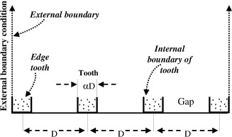
Figure 1: Teeth and gaps covering space.

The microscopic simulation operates on the position of each particle. We are interested in a meaningful coarse description, a finite-dimensional approximation to the density of particles, $u(x)$, possibly averaged over several realizations of the computational experiment Kevrekidis02 . The lifting operator that maps a given $u(x)$ to consistent particle positions is straightforward in this case. From the density function over a tooth we can compute its integral, so we know the number of particles that should be present in that tooth. The indefinite integral of the density function over the tooth provides the cumulative distribution function for that tooth which permits the particles to be placed as a discrete representation of that functioncwgdist . If the density approximation is constant in each tooth (as has been found to be adequate in the examples here) this simply means that the particles are uniformly spaced in each tooth according to the density in that tooth.

In our particular stochastic simulation, the evolution rules require a local density estimate. This should be done by choosing a particle density influence function $\sigma(d)$ that specifies the contribution of each particle to the local density at a distance $d$ from that particle. If this function is constant for $d<w$ and zero elsewhere, the local density function at $x$ is found by just counting the number of particles within distance $d$ of $x$. Ref. Chertock01 ; Chertock02 , seeking some level of differentiability, use a Gaussian spreading function for each particle. Since we do not require differentiability, we will count particles within distance $d$. By making $d$ twice the tooth size, we can then simply count the particles in each tooth. We have also used higher-order approximations, but it is not clear that they yield sufficient improvements in accuracy to justify the additional computational effort. The technique used for higher-order approximations is based on the fact that the sample cumulative distribution function in each tooth is known from the particle positions. We can then fit a polynomial to it within each tooth. The density function over a tooth is simply given by the derivative of this polynomial.

The mapping of a phase point or points (particle positions and velocities history) to coarse fields is called a restriction operator. In addition to the density field ($0$th-moment), smooth velocity ($1$st-moment) and temperature ($2$nd-moment) fields can be extracted from molecular dynamics based on maximum likelihood inference Li98 . If the interior of a tooth were to be simulated by solving a PDE, we would need to prescribe appropriate boundary conditions at each tooth at each timestep. The same is still true when the tooth is realized using particle-based microscopic simulations. Creating an appropriate match between the coarse fields at the boundaries and the particles in the teeth is an area of intense researchLi99 ; E01 . Sometimes one knows so little about the nature of the coarse equation that even the correct order for imposing well-posed boundary conditions at the teeth is unknown. This issue is addressed in Li03 .

Here we use an alternative approach suggested in Gear02b . In a 1D particle based random walk simulation we can distinguish two “fluxes” - left-going and right-going. The particle simulation in the interior of each tooth generates outgoing fluxes, that is, the left[right]-going fluxes at the left[right] boundaries, directly. Boundary conditions are needed to provide matching incoming (right[left]-going) fluxes at the same boundaries. In $d$-dimensions, there will be $2^{d}$ boundaries to deal with and the corresponding incoming fluxes to provide.

Consider the estimation of the right-going incoming flux, ${\rm I}_{r,1}$, as shown in Fig. 2.

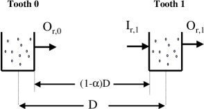
Figure 2: Right-going Input and Ouput Fluxes

Assuming macroscopic flux smoothness suggests that we can interpolate its values from neighboring outgoing fluxes, in this case ${\rm O}_{r,0}$ and ${\rm O}_{r,1}$. If we use linear interpolation, we can write

$${\rm I}_{r,i}=\alpha{\rm O}_{r,i-1}+(1-\alpha){\rm O}_{r,i}.$$ (2)

The interpolation coefficients depend (in this case through $\alpha$) only on the gap-tooth geometry.

However, the “fluxes” under discussion here are not real-valued quantities, but discrete events as particles cross a boundary, so Eq.(2) needs a different interpretation. Consider instead the role played by each outgoing flux in the interpolation for ingoing fluxes. An interpretation of Eq.(2) for $i=1$ and $i=2$ would be the portion $(1-\alpha)$ of ${\rm O}_{r,1}$ contributes to the flux ${\rm I}_{r,1}$ while $\alpha$ of it contributes to ${\rm I}_{r,2}$. A similar procedure applies to the left-going fluxes. Thus, rather than thinking in terms of flux interpolation we can think in terms of flux redistribution. Interpreting the linear interpolation stochastically, (on a regularly spaced gap-tooth scheme) we direct $\alpha$ of the outgoing particles as input to the neighboring tooth, and redirect $(1-\alpha)$ of them back to the other boundary of the same tooth as shown in Fig. 3.

Flux redistribution has to recognize the position of a particle after it leaves a tooth. If it had moved to a distance $\delta$ beyond the boundary of the tooth, it must be inserted a distance $\delta$ inside the receiving tooth. If $\delta$ were larger that the tooth width it would have left a tooth boundary again and a further redistribution would be required following the same rule. (In multiple dimensions, the boundaries in each dimension are treated independently so that a particle will be distributed for each boundary that it crosses until it is inside a tooth.)

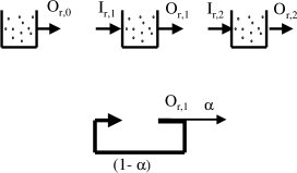
Figure 3: Flux Redistribution for Right-going Fluxes

The above method implements effective linear interpolation. As discussed in Gear02b , linear interpolation is not adequate for second-order problems: at least quadratic interpolation must be used. A possible quadratic interpolation formula is

$${\rm I}_{r,i}=\frac{\alpha(1+\alpha)}{2}{\rm O}_{r,i-1}+(1-\alpha^{2}){\rm O}_{r,i}-\frac{\alpha(1-\alpha)}{2}{\rm O}_{r,i+1}.$$

As before we consider the impact of each outgoing flux on incoming fluxes. The fractions of output ${\rm O}_{r,1}$ should be sent to the inputs as follows: $(1-\alpha^{2})$ to ${\rm I}_{r,1}$; $\alpha(1+\alpha)/2$ to ${\rm I}_{r,2}$: and $-\alpha(1-\alpha)/2$ to ${\rm I}_{r,0}$.

Note that the last value is negative. Any linear higher-order interpolation formula contains negative coefficients. Our solution is to direct anti-particles to the appropriate teeth. There they must annihilate with regular particles - we simply annihilate with the nearest regular particle. With this approach, the ${\rm O}_{r,1}$ is redistributed as follows: $(1-\alpha(1+\alpha)/2)$ to ${\rm I}_{r,1}$; $\alpha^{2}$ to ${\rm I}_{r,2}$; and $\alpha(1-\alpha)/2$ are cloned to get two regular particles sent to ${\rm I}_{r,1}$ and ${\rm O}_{r,2}$ and one anti-particle sent to ${\rm I}_{r,0}$ It is interesting to observe that this scheme conserves the total number of particles in the computation.

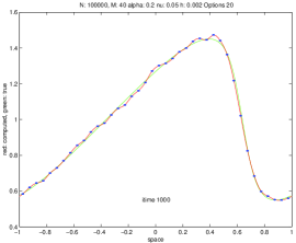
(a)

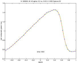
(b)

Figure 4: Simulation results after 1,000 steps. $\alpha=0.2$. (a) 100,000 particles (b) 500,000 particles

The microscopic evolution rules were simulated at conditions corresponding to $\nu=0.05$ and timestep $h=0.002$ in Eq.(1) for 1,000 time steps using the gap-tooth scheme with 40 equally spaced teeth in the interval $[-1,1)$. The tooth-to-spacing ratio was $\alpha=0.2$. The coarse initial condition was $1-\sin(\pi x)/2$. Fig. 4 shows the results at $t=2$ when 100,000 particles are used (upper figure) and 500,000 particles (lower figure). The dots indicate the particle density approximations within each tooth (constant in this case); they are connected by a spline interpolant. The smooth curve (to guide the eye) is the analytical solution Cole51 ; Hopf50 of Eq.(1).

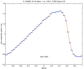
Figure 5: Standard particle simulation (no gaps)

The problem was also run with $\alpha=1$, i.e., no gaps, to compare with a conventional, full space, direct microscopic simulation. Fig. 5 shows the result using 500,000 particles and a constant density approximation in each tooth. This is the same average particle density per spatial unit as with $\alpha=0.2$ and 100,000 points. The results are comparable. The $\alpha=1$ case with 40 teeth and 500,000 particles has also been run with the polynomial density interpolants described above of degrees 1 and 2. No significant difference in the solutions were observed, and neither were differences observed when the higher order polynomial fits were used with $\alpha=0.2$.

We have demonstrated that the gap-tooth scheme can be successful in solving some problems using microscopic models based on the stochastic simulation of particle motion; we also introduced a novel approach for dealing with the inter-tooth boundary conditions.

In earlier work we have proposed combining this with projective integration Gear01a and some preliminary experiments have been performed in this direction. However, projective integration requires smoothness of the time derivative estimates. The stochastic nature of the microscopic model leads to significant noise. In this simulation we used a least-squares linear estimate from a large number of time steps to get a reasonably accurate time derivative estimate. However, by then, the total time step at the microscopic level was large relative to the size of a projective step in time (which is limited by the smoothness of the solution). If the stochastic noise is reduced by using a much larger number of particles, or a large number of “copies” of the simulation, the time derivative estimates would allow the application of projective integration. In some sense there is a tradeoff between saving computation in the spatial domain with fewer teeth and fewer particles, and saving computation in the time domain by getting more accurate estimates of the time derivatives. We believe that for problems where there is a significant gap between the timescales of the microscopic dynamics and those of the expected macro-scale behavior, projective intregration would be a useful addition. We will report on such “patch dynamics” experiments in a future paper.

This work was partially supported by the Air Force Office of Scientific Research (Dynamics and Control) and an NSF ITR grant (C.W.G.,I.G.K.). J.L. acknowledges support by Honda R&D Co., Ltd. (RF# 744252) and the OSU Transportation Research Endowment Program.

References

- (1) I.G. Kevrekidis, C.W. Gear, J.M. Hyman, P.G. Kevrekidis, O. Runborg, C. Theodoropoulos, submitted to Communications in the Mathematical Sciences.
- (2) J. Li, K.J. Van Vliet, T. Zhu, S. Yip, S. Suresh, Nature 418 (2002) 307-310. K.J. Van Vliet, J. Li, T. Zhu, S. Yip, S. Suresh, Phys. Rev. B 67 (2003) 1041XX.
- (3) R. Phillips, D. Rodney, V. Shenoy, E. Tadmor and M. Ortiz, Model. Simul. Mater. Sci. Eng. 7, 769 (1999).
- (4) I.G. Kevrekidis, Plenary Lecture, CAST Division, AIChE Annual Meeting, Los Angeles, 2000. Slides can be obtained at http://arnold.princeton.edu/yannis/
- (5) C.W. Gear, I.G. Kevrekidis, to appear SIAM Journal on Scientific Computing.
- (6) C.W. Gear, I.G. Kevrekidis, C. Theodoropoulos, Computers and Chemical Engineering 26 (2002) 941-963.
- (7) C.W. Gear, NEC Research Institute Report TR 2001-130, Nov, 2001.
- (8) A. Chertock, D. Levy, J. Comp. Phys. 171 (2001) 708-30.
- (9) A. Chertock, D. Levy, J. Sci. Comp. 17 (2002) 491-499.
- (10) J. Li, D. Liao, S. Yip, Phys. Rev. E 57 (1998) 7259-7267.
- (11) J. Li, D. Liao, S. Yip, J. Comput.-Aided Mater. Des. 6 (1999) 95-102.
- (12) W. E, Z. Huang, Phys. Rev. Lett. 87 (2001) 135501.
- (13) J. Li, P.G. Kevrekidis, C.W. Gear, I.G. Kevrekidis, submitted to Multiscale Modeling and Simulation. http://arxiv.org/abs/physics/0212034
- (14) C.W. Gear, I.G. Kevrekidis, NEC Research Institute Report TR 2002-031N, Oct. 2002. http://arXiv.org/abs/physics/0211043
- (15) J.D. Cole, Quart. Appl. Math. 9 (1951) 225-236.
- (16) E. Hopf, Comm. Pure Appl. Math. 3 (1950) 201-230.