Abstract

We analyze the stability of a cylindrical Couette flow under the imposition of a weak axial flow in case of a very short cylinder with a narrow annulus gap.

We consider an incompressible viscous fluid which is contained in the narrow gap between two concentric short cylinders, where the inner cylinder rotates with constant angular velocity. The caps of the cylinders have narrow tubes conically tapering to super narrow slits which allow for an axial flow along the surface of the inner cylinder.

The approximated solution for the Couette flow for short cylinders was found and used for the stability analysis instead of the exact but bulky solution. The sensitivity of the Couette flow to general small perturbations and to the weak axial flow was studied. We demonstrate that perturbations coming from the axial flow cause the propagation of dispersive waves in the Taylor-Couette flow.

The coexistence of a rotation and of an axial flow requires to study in addition to the energy and the angular momentum also the helicity of the flow. The approximated form for the helicity formula in case of short cylinders was derived.

We found that the axial flow stabilizes the Taylor - Couette flow. The supercritical flow includes a rich variety of vortical structures including a symmetric pair of Taylor vortices, an anomalous single vortex and quasi periodic oscillating vortices. Pattern formation was studied at large for rated ranges of azimuthal and axial Reynolds numbers. A region where three branches of different states occur was localized. Numerical simulations in 3D and in axisymmetrical case of the model flow are presented, which illustrate the instabilities analyzed.

Key words and phrases: Taylor-Couette flow, stability under axial flow, pattern structures
PACS numbers: 47.32.-y, 47.20.-k, 47.54.+r

1 Introduction

Since the famous experiments of Taylor [1] in long cylinders many experimental and theoretical investigations of the interesting phenomena of arising and evolution of Taylor vortices were done. The main part of these studies was devoted to cases of long cylinders. It was done under the assumption that a sufficiently long cylinder and periodic boundary conditions will emulate the infinitely long cylindrical region well. In addition such regions are convenient for theoretical investigations. The experimental investigations of short cylinders started much later and gave surprising results (see, for example, Benjamin and Mullin [2]), which indicated that the zone and the magnitude of the influence of the caps of the cylinders is much bigger and takes effect on the type of motion in the whole region. It was assumed that close to the caps of the cylinders the boundary layer is directed from the outer to the inner cylinder as a result of the existence of an Ekmans boundary layer. However, the experiments gave a more complicated picture of the motions. There exists also an atypical layer in opposite direction, i.e. from the inner to the outer cylinder connected withe the existence of the ’anomalous mode’. The first mathematical model which took the influence of the cylinder caps into account was represented in the work of Schaeffer [3]. This model is not very consistent and needs improvements. The role of the anomalous mode was studied later numerically and experimentally in the works of Cliffe et al [4], [5]. The transient features of the circular Couette flow were investigated in laboratory and numerical experiments (using the commercial program ’Nekton’ (Fluent GmbH) by Neitzel et al [6]. The results of the numerical experiments were close to the laboratory experiments. In case of short cylinders with an aspect ratio $\Gamma\sim 1$ (relation of annulus span to the annulus gap width, defined in section 2) usually only one pair of Taylor vortices arises. In general, this case is considered to be not really interesting due to the poorness of the patterns to be expected. But in the experiments of Aitta et al [7] a series of interesting flow patterns for short cylinders was found. A non-equilibrium tricritical points occurs when a forward bifurcation becomes a backward bifurcation. In the Taylor - Couette problem the tricritical point can be observed for $\Gamma_{T}=1.255$ in the classical case of a pure rotation of the inner cylinder without axial flow as demonstrated in [7] and later in [8]. The system of two vortices is symmetrical if the rotation velocity does not exceed a critical velocity $v_{1}.$ If the velocity of the flow is larger, $v>v_{1}$, then one vortex grows at the expense of the other one. In the case of the forward bifurcation the symmetry is broken continuously and in the case of the backward bifurcation - abruptly. In the phase transition language this is a bifurcation of the second order or first order correspondingly [9]. The continuous transition was observed for $\Gamma<\Gamma_{T}$ and the abrupt one for $\Gamma_{T}<\Gamma<\Gamma_{C},$ where $\Gamma_{C}=1.292.$

An exhaustive study of the influence of the finite length effects is done for the classical arrangement of two concentric cylinders with a very small aspect ratio $\Gamma\in[0.5,1.6]$ and a relatively large annulus with a radius ratio (relation between the radii of inner and outer cylinders, see section 2) of $\eta=0.667$ for moderate Reynolds numbers $Re\in[100,1500]$ in the work of Furukava, Watanabe, Toya & Nakamura [10] in the case when the inner cylinder is rotating. The numerical investigations were verified by experiments. The three main flow patterns were found which correspond to a normal two-cell mode, an anomalous one-cell mode and a twin - cell mode. A steady case as well as an unsteady mode of the fully developed flow different from wavy Taylor - Couette flow were obtained.

There exists a series of experimental and theoretical works devoted to the linear stability of the Taylor-Couette problem with implosed axial effects. The first such analysis was done for the case of axisymmetric disturbances in a narrow gap [11], [12]. In the work of Marques and Lopez [13] the linear stability of the flow in the annulus between two infinitely long cylinders, driven by a constant rotation and harmonic oscillation in the axial direction of the inner cylinder was analyzed using Floquet theory. The axial effects in the Taylor-Couette problem were studied in the work [14] on two different flows. In the first one the axial effect is introduced by an inertial axial sliding mechanism between the cylinders and in the other one via an imposed axial pressure gradient. In all cases the annular gap is much larger as in our case and the radius ratio is $\eta=0.5,~{}\dots,~{}0.8.$ The stabilizing effect of a periodical axial flow was studied in the works [15], [16] and [17]. In the work of Lueptow [18] the stability problem of a Taylor-Couette flow with axial and radial flow was studied for a relatively large radius ratio $\eta=0.83$ and pressure-drive axial flow in the whole annulus. In all these studies it was found that the axial flow stabilized the Taylor-Couette flow and enables a lot of super critical states with a rich variety of patterns.

Nevertheless the theory of the Taylor - Couette flow is by far from being complete, so for instance the stability problem for the system of Taylor vortices and a classical Couette flow by influencing control of the cylinder caps. It is also a little bit astonishing that the exact analytical solution for the Couette flow profile with boundary conditions on cylinder caps was obtained only recently in the work of Wendl [19]. His results expose a strong influence of the caps on the flow profile. The difference between the two profiles with and without finite-length effects is approximately a logarithmic function of the aspect ratio $\Gamma$ for a wide range of radius ratios $\eta$. The solution is given in form of a slowly convergent series which contains trigonometric and Bessel functions. To give a qualitative analysis of instabilities one takes an exact solution as a base flow to linearize the Navier - Stokes equations. This type of solutions is not convenient to pursue the topic further towards analytical studies of the instabilities.

In the present work we use the theory of small perturbations to study the instability of the laminar Couette flow in a short cylinder. The geometry of an annular gap and the boundary conditions are given in the section 2. Our idea was to get an analytical formula which is simpler than that in [19] but which gives us an approximation of the Couette flow with finite-length effects which is as good as that found in [19]. In the section 3 we describe this solution and discuss the region of applicability of the done approximation.

The solution obtained for a short cylinder is well suitable as a base flow for a comprehensive study of instability effects. This study is represented in the section 4. The onset of the instability is predicted using the method of local analysis, in which the equations governing the flow perturbation are linearized. For the very reason that the appearance of an instability depends not only on the base flow but also on the amplitude and the type of the flow perturbation two different types of perturbations are studied in this section. We consider the sensitivity of the Couette flow under small perturbations corresponding to an axial flow which is the most important for industrial applications. We take the case of a very narrow annulus $\eta\sim 1$ which is typical for bearing or sealing systems and in contrary to general expectation we get a rich family of flow states. We proved that the axial flow stabilizes the Taylor - Couette flow also in case of very short cylinders and narrow annular gap with axial flow directed as a thin layer along the surface of the inner rotating cylinder.

The elaborate series of the numerical experiment was done with help of the FLUENT 5.5/6.0. The detailed description of the grids used and others numerical facilities is given in the section 6.

The change from one laminar flow to another or a transition from a laminar flow to turbulence is a function of the base flow considered as well as of the type of small perturbations. We found a rich family of typical patterns on large intervals of Reynolds numbers. The results of the numerical experiments are discussed in the section 7.

2 The main problem

The study of the Couette - Taylor problem for the parameters defined below was stimulated by the industrial project [22]. In many technical systems the problem of transmitting energy and momentum is solved using shafts and corresponding bushes with or without radial sealing. In a typical situation one is concerned with a small Taylor-Couette annulus, narrow slits in between cylinders and with axial and tangential oscillations or with a weak axial flow along the surface of the inner cylinder. In general, these systems are very complicated and it is necessary to study more simple problems in order to isolate a particular mechanism and to develop and test hypotheses governing their behavior. We separate here only one of the most typical cases because of its technological importance and, from a fundamental point of view, for its rich dynamics and try to describe all possible flow states in this case.

We consider the motion of the fluid in an annulus between two cylinders as represented in fig. 1.

Figure 1: The geometry of the annulus. The radii of the inner and outer cylinders are equal to $r_{in},r_{out}$ correspondingly, the annulus span is denoted by $l,$ the annular gap width is $d=r_{out}-r_{in}.$ The corresponding geometrical parameters of the slits are denoted by $\tilde{d}$ and $\tilde{l}.$ Other notations are explained in the text.

The annulus dimensions are the gap width $d$, the annulus span $l$, the radius of the inner cylinder $r_{in}$, the of an outer cylinder $r_{out}$. The corresponding dimensionless geometric parameters are the aspect ratio $\Gamma=\frac{l}{d}$ and the radius ratio $\eta=\frac{r_{in}}{r_{out}}$. We use these notations during the whole paper. For many sealing or bearing systems $\Gamma\sim 1$ and $\eta\sim 1.$ We fixe in all our calculations $\Gamma=1.02$, $\eta=0.95356~{}.$

We assume that the inner cylinder to turn at the constant rate $\omega.$ The outer cylinder is at rest, the axial flow has a constant velocity $w_{0}$ and we suppose $r_{in}\omega\gg w_{0}.$ The equations of fluid motion and boundary conditions will be rendered dimensionless using $d,$ as a unit for length. The radius of the inner cylinder will be denoted by $R=\frac{r_{in}}{d}$ in dimensionless units which will be used in all sections of this paper.

The entrance way and the outgoing way for the axial flow are very thin cylindrical slits with the gap width $\tilde{d}$ and the annulus span of slits denoted by $\tilde{l}.$ The slits are long and narrow in comparison to the main annulus i.e. $l\sim\tilde{l},$ $d\gg\tilde{d}.$ The ends of the slits narrow conical to the lower order of scale that means the most narrow part of the slit has the width $\widetilde{\widetilde{d}},$ which is very small, $d\gg\tilde{d}\gg\widetilde{\widetilde{d}}$. A more detailed picture of the slits is given in fig. 7. The studied flow states are very sensitive to the kind of perturbations. So we try to construct a situation which is most adapted to technical facilities and imitate the sealing arrangements with conical tapering slits.

It is characteristically for quite all technical applications that the sealing medium is oil with non vanishing viscosity. We will consider in our work an incompressible viscous fluid in the cylindrical annulus.

3 An approximation of the exact solution in case of the rotating inner cylinder

The classical case of the Couette flow of an incompressible viscous fluid in an annulus between two cylinders was investigated analytically in [19]. In comparison to the famous work of Taylor the author studied cylinders of a finite length and got a much more complicated formula which describes the influence of the cylinder caps on the flow. As follows from experiments of Kageyama ([20]) if the Reynolds number grows the influence of the Ekmans layer drops along the cylinder caps. As a result the profile of the solutions differs more and more from the pure Couette solution because of the arising of secondary flows in the annulus.

We will consider the flow in the annular gap with the width $d,$ the span $l,$ and radius of inner cylinder $r_{in}$ as on the fig. 1 without slits. We suggest now that the caps of the cylinders contact the inner cylinder and that there is no axial flow in the annulus. The equations of the fluid motion and the boundary conditions will be rendered dimensionless using $v=r_{in}\omega$ and $P=(\nu/d)^{2}$ as units for velocity and the pressure. The scaling of the velocities and of other quantities will change from section to section.

Due to the axial symmetry two of the components of the velocity vector ${\bf u}(r,\theta,z)$ vanish in this case and the velocity vector reads

$${\bf u}(r,z)=(0,V_{0}(r,z),0),$$ (1)

where $V_{0}(r,z)$ is the azimuthal component. The cylindrical Navier-Stokes equations can be reduced in this model to one equation,

$$\frac{\partial^{2}V_{0}}{\partial r^{2}}+\frac{1}{R+r}\frac{\partial V_{0}}{\partial r}-\frac{V_{0}}{(R+r)^{2}}+\frac{1}{\Gamma^{2}}\frac{\partial^{2}V_{0}}{\partial z^{2}}=0.$$ (2)

The boundary conditions can be rendered dimensionless as

$$V_{0}(r,0)=0,~{}~{}V(r,1)=0,~{}~{}V_{0}(0,z)=1,~{}~{}V_{0}(1,z)=0,~{}z\in[0,1],~{}r\in[0,1].\\$$ (3)

We make an additional scaling in $z-$direction by $\Gamma$ to reach the more convenient situation that the both variables $r$ and $z$ lie in the interval $[0,1].$ The considered case was solved by Wendl [19] using the Fourier transformation. The solution has the following form

$$V_{0}(r,z)=$$ (4)

$$\frac{1}{4\pi}\sum_{m=1}^{\infty}{\frac{\left(I_{1}(\beta_{m}(R+1))K_{1}(\beta_{m}(R+r))-K_{1}(\beta_{m}(R+1))I_{1}(\beta_{m}(R+r))\right)\sin(\beta_{m}z)}{(2m-1)\left(I_{1}(\beta_{m}(R+1))K_{1}(\beta_{m}R)-K_{1}(\beta_{m}(R+1))I_{1}(\beta_{m}R)\right)}}$$

with $\beta_{m}=\frac{(2m-1)\pi}{\Gamma}$. Here $I_{1}$ and $K_{1}$ are modified Bessel functions. This solution differs from Taylor-Couette’s simple linear solution especially strong in cases of short cylinders but remains an exact solution for long cylinders. The series in (4) converges very slowly and it is difficult to use it for the intended analytical studies. This was the reason that we looked for simpler analytical representations of this solution or for some good approximated solution.

We study the case of short cylinders, i.e. $\Gamma\sim 1,$ with a narrow gap, $\eta\sim 1$, and $R\gg 1.$ Under these assumptions and taking into account $r\in[0,1]$ we can simplify the initial equation (2) by replacing $\frac{1}{R+r},\frac{1}{(R+r)^{2}}$ by the constants $\frac{1}{R},\frac{1}{R^{2}}.$ For the simplified equation which has constant coefficients we obtain the solution in closed analytical form,

$$V_{0}(r,z)={\frac{2}{\pi}}\arctan\left(\left(\sinh^{-1}\left(\frac{\pi}{\Gamma}r\right)-\sinh^{-1}\left(\frac{\pi~{}}{\Gamma}\left(2-r\right)\right)\right)\sin(\pi z)\right)$$ (5)

for $r\in[0,1]$ and $z\in[0,1]$. This is a convenient form of the approximated solution for the fundamental mode of the Couette flow profile which we will use in the following.

The agreement between the approximated and the exact solutions is very good as can be seen from fig. 2.

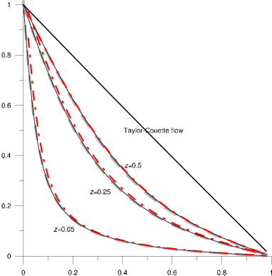
a). $R=20,$

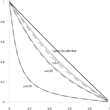
b). $R=10,$

Figure 2: The profiles $V_{0}(r,z)$ of the exact (dashed line), the approximated solutions (continous line) and numerical solution (dash-dotted line) on $z-$levels equal to $z=0.05,0.25,0.5$ with $\Gamma=1$ as functions of $r.$ The numerical solution was found with program FLUENT 5.5/6.0 in axisymmetric case for $\mbox{Re}=100.$

The approximated solution (5) is stable for small Reynolds numbers $Re$ and can be used as a base state in a stability analysis.

We note an earlier attempt by Vladimirov [21] to find an approximative solution which takes the influence of the caps into account , which, however, differs much more from the exact solution than ours.

4 Stability problem for the Taylor - Couette flow under small perturbations

4.1 Local stability study for a short cylinder

We consider the axisymmetrical stability problem of the Taylor-Couette flow. We assume that the velocity vector $\mathbf{\tilde{u}}(r,z)$ which describes the fluid motion in the annular gap like on the fig. 1 can be represented as a sum of two vectors $\mathbf{u}(r,z)=(u,v,w)$ and $\mathbf{{v}}(r,z)=(0,V_{0},0)$

$$\mathbf{\tilde{u}}(r,z)=\mathbf{{v}}(r,z)+\mathbf{u}(r,z)=(0,V_{0},0)+(u,v,w),$$ (6)

where $V_{0}$ describes the fundamental mode of the Couette flow and $\mathbf{{u}}(r,z)$ a perturbation of this mode. We assume also that the pressure $\tilde{P}$ can be also represented as sum $\tilde{P}=P_{0}+p.$

Under the following assumptions

$$\max_{r,z}|\mathbf{{v}}(r,z)|\gg\max_{r,z}|\mathbf{u}(r,z)|,~{}~{}\max_{r,z}{\frac{|\nabla\mathbf{u}|}{|\mathbf{u}|}}\gg\max_{r,z}{\frac{|\nabla\mathbf{{v}}|}{|\mathbf{{v}}|}},$$ (7)

where $\nabla$ denotes the spatial gradient of the corresponding velocity, the system of the Navier-Stokes equations can be linearized. The linearized Navier-Stokes equations (LNSE) in the axisymmetrical case take the form

$$\partial_{t}u-2\operatorname{Re}\frac{vV_{0}}{R+r}=-\partial_{r}p+\Delta u-\frac{u}{\left(R+r\right)^{2}},$$ (8)

$$\partial_{t}v+\operatorname{Re}\left(\partial_{r}V_{0}u+\frac{V_{0}}{R+r}u+\partial_{z}V_{0}w\right)=\Delta v-\frac{v}{\left(R+r\right)^{2}},$$

$$\partial_{t}w=-\frac{1}{\Gamma^{2}}\partial_{z}p+\nu\Delta w,$$

$$\partial_{r}u+\frac{u}{R+r}+\partial_{z}w=0,$$

where $\Delta$ is the Laplace operator,

$$\Delta=\partial_{rr}+\frac{\partial_{r}}{R+r}+\frac{\partial_{zz}}{\Gamma^{2}}.$$ (9)

The Reynolds number is $\operatorname{Re}=\frac{\omega r_{in}d}{\nu}$ and $\nu$ denotes the viscosity of the fluid. The dimensionless variables $r,z$ describing the flow in the cylindrical annulus belong to the intervals

$$r\in\left[0,1\right],~{}~{}\ z\in\left[0,1\right].$$ (10)

Here we use the dimensionless variables as introduced in the section 2 and additionally we use the value $d^{2}/\nu$ and $R\omega$ to render time and velocities dimensionless too. We leave the same notations for the velocities in the dimensionless case as above. It means that now $|V_{0}|\sim 1$ and from the conditions (7) $|v|\ll 1$ follows.

Let’s introduce a stream function $\Psi$ as usual in the axisymmetrical case [23]

$$u=\frac{\partial_{z}\Psi}{R+r},~{}~{}w=-\frac{\partial_{r}\Psi}{R+r}.$$ (11)

In terms of the stream function $\Psi$ and the azimuthal velocity $v$ the LNSE (8) turns into a system of two coupled equations

$$\partial_{t}\widetilde{\Delta}\Psi-\frac{\operatorname{Re}}{\Gamma^{2}}\left(\frac{2\partial_{z}V_{0}}{R+r}v+\frac{2V_{0}}{R+r}\partial_{z}v\right) = \Delta\widetilde{\Delta}\Psi-\frac{\widetilde{\Delta}\Psi}{\left(R+r\right)^{2}},$$

$$\partial_{t}v+\operatorname{Re}\left(\left(\partial_{r}V_{0}+\frac{V_{0}}{R+r}\right)\frac{\partial_{z}\Psi}{R+r}-\partial_{z}V_{0}\frac{\partial_{r}\Psi}{R+r}\right) = \Delta v-\frac{v}{\left(R+r\right)^{2}}.$$ (12)

We remark that the value $\widetilde{\Delta}\Psi$ is an azimuthal vorticity ${\Upsilon}_{\theta}$ defined by

$${\Upsilon}_{\theta}=\widetilde{\Delta}\Psi=\frac{1}{\Gamma^{2}}\partial_{z}u-\partial_{r}w,~{}~{}{\rm where}~{}~{}\widetilde{\Delta}=\frac{\Delta}{R+r}.$$ (13)

The basic Taylor-Couette flow is an axial inhomogeneous flow in the case of the short cylinder because of the cylinder caps influence. The inhomogeneity leads to additional terms which make a difference between the system (8) and the corresponding linearized Navier-Stokes equations for an infinitely long cylinder. Now we will prove that the additional terms causes the propagation of dispersive waves in the Taylor - Couette flow.

We remember that in the case of a short cylinder with very narrow gap we have

$$\Gamma\sim 1,~{}~{}\eta\sim 1,~{}~{}R\gg 1.$$ (14)

Under these assumptions we can simplify the system of equations (12) by replacing the coefficients $\frac{1}{(R+r)^{n}}$ (note $r\in[0,1]$) by the constants $\frac{1}{R^{n}},~{}n=1,2.$ The operators $\partial_{z}$ and $\partial_{r}$ can be replaced by the multiplicative operators $\partial_{r}\sim 1/d,~{}~{}\partial_{z}\sim 1/l$ or, in the dimensionless case, by

$$\frac{\partial}{\partial r}\sim 1,~{}~{}\frac{\partial}{\partial z}\sim\frac{1}{\Gamma}$$ (15)

because of the relations (10) and (14). Furthermore we assume

$$\frac{\partial V_{0}}{\partial r}\gg\frac{V_{0}}{R+r}$$ (16)

and neglected $\frac{V_{0}}{R+r}$ in the system (12). We collect now the leading terms of the system (12) only and obtain a simplified system of equations

$$\partial_{t}\Delta\Psi-2\operatorname{Re}\partial_{z}V_{0}v-2\operatorname{Re}V_{0}\partial_{z}v = \Delta^{2}\Psi,$$ (17)

$$\partial_{t}v+\delta\operatorname{Re}\partial_{r}V_{0}\partial_{z}\Psi-\delta\operatorname{Re}\partial_{z}V_{0}\partial_{r}\Psi = \Delta v,$$

where no-slip boundary conditions $u|_{S}=v|_{S}=w|_{S}=0$ on the inner surface $S$ of the annulus are adopted. In the system (17) we denoted $\Delta=\partial_{rr}^{2}+\frac{1}{\Gamma^{2}}\partial_{zz}^{2}$, and the constant $\delta\equiv\frac{1}{R}$ is small, $\delta<<1$.

The standard, straightforward way to investigate the stability problem would consist in finding the exact solution of the eigenvalue problem corresponding to the system of equations (17). Then the perturbations ${\bf u}(r,z)$ can be represented as a series over the eigenfunctions. Alternatively, the system could be solved numerically whereas a spatial discretization of the problem may be accomplished by a solenoidal Galerkin scheme. In our case these procedures may be accomplished numerically only and this is outside the scope of the present work.

Nevertheless we can give good qualitative characteristics of the flow in the annulus if we use a local stability analysis. This method was first developed in the analysis of an inhomogeneous complex astrophysical flow [24],[25]. It give us the possibility to establish the main physical processes of the considered fluid flow system [26], [27].

The main idea of the local stability analysis method also named a method of infinitesimal perturbations can be described as follows. We suppose that the amplitude and the gradients of the main state (the fundamental mode of the Couette flow in our case) is preserved under the perturbations. This means we keep the values $V_{0},\partial_{z}V_{0}$ and $\partial_{r}V_{0}$ unaltered or assume that they are constant. For all components of the perturbation vector ${\bf u}(r,z)=(u,v,w)$ and their derivatives Taylor series are used which are truncated after the first two terms. From the physical point of view we assume that the perturbation scale is much smaller than the typical scale of the axial inhomogeneity in the Taylor-Couette system. This is the locality condition. As usual we represent the perturbation as a plain wave,

$$\Psi\sim\widehat{\Psi}\exp\left(\gamma t+i\left(k_{r}r+k_{z}z\right)\right),~{}~{}v\sim\widehat{v}\exp\left(\gamma t+i\left(k_{r}r+k_{z}z\right)\right),$$ (18)

where $\widehat{\Psi}$ and $\widehat{v}$ are the amplitudes of the waves. The vector of wave numbers $k=(k_{r},k_{z})$ defines the spatial direction of the plane wave propagation. The locality condition requires that $k_{r},k_{z}\gg 1.$ In (18), $\gamma$ has the dimension of a frequency and in the stability analysis it is called the time increment (or simply increment). In the case of an intrinsic instability of the investigated system $\gamma$ will be positive. This means that the amplitude of the plane wave will infinitely increase with time. This is the unstable case.

The substitution of the plane wave (18) into the linearized system (17) results in a system of algebraic equations for the increment $\gamma$,

$$-k^{2}\left(\gamma+k^{2}\right)\widehat{\Psi}-2\frac{\operatorname{Re}}{\Gamma^{2}}\left(\partial_{z}V_{0}+iV_{0}k_{z}\right)\widehat{v} = 0,$$

$$\left(\gamma+k^{2}\right)\widehat{v}+i\delta\operatorname{Re}\left(\partial_{r}V_{0}k_{z}-\partial_{z}V_{0}k_{r}\right)\widehat{\Psi} = 0,$$

where $k^{2}=k_{r}^{2}+\Gamma^{-2}k_{z}^{2}.$ This system can be solved explicitly and we obtain two solutions for the increment $\gamma$,

$$\gamma_{\pm}=-k^{2}\pm\frac{\operatorname{Re}\left(2\delta\right)^{1/2}\left|k_{z}\partial_{r}V_{0}-k_{r}\partial_{z}V_{0}\right|^{1/2}}{\Gamma k}\left(k_{z}^{2}V_{0}^{2}+\left(\partial_{z}V_{0}\right)^{2}\right)^{1/4}\times$$

$$\times\left(\cos\left(\frac{1}{2}\arctan\left(\frac{\partial_{z}V_{0}}{k_{z}V_{0}}\right)\right)-i\sin\left(\frac{1}{2}\arctan\left(\frac{\partial_{z}V_{0}}{k_{z}V_{0}}\right)\right)\right).$$ (19)

As a consequence, in the system two different regimes of motion can exist.

The motion in the annulus is strong inhomogeneous in $z-$direction because of the influence of the cylinder caps. Let us now look for local increments on the middle surface $r=0.5$ on three different lines $z=0.25,~{}0.5,~{}0.75~{}.$ For $z=0.5$ the increment does not have any imaginary part and on this line the system does not show any oscillations. In this case the real part of the increment is represented in fig. 5. On the lines $z=0.25,~{}0.75$ the increment has an imaginary part and the system has oscillations with frequencies which are directly proportional to the gradient of the undisturbed state.

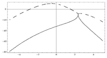
Figure 3: The real part $Re\gamma(k_{r})$ of the increment $\gamma$ as a function of $k_{r}$ for $z=0.25,~{}$ $r=0.50,$ $k_{z}=-2.00,$ $\hbox{Re}=110.$

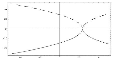
Figure 4: The imaginary part $Im\gamma(k_{r})$ of the increment $\gamma$ as a function of $k_{r}$ for $z=0.25,~{}$ $r=0.50,$ $k_{z}=-2.00,$ $\hbox{Re}=110.$

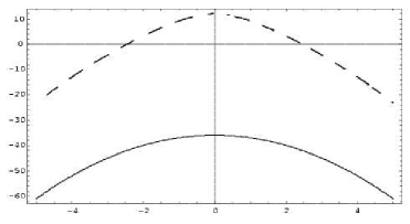
Figure 5: The real part $Re\gamma(k_{r})$ of the increment $\gamma$ as a function of $k_{r}$ for $z=0.50,~{}$ $r=0.5,~{}$ $k_{z}=-2.0,$ $\hbox{Re}=110.$

For $\partial_{z}V_{0}=0$ we have two real solutions for the increment and, consequently, two branches of non-oscillating solutions.
The two branches of the increment given by Eq.(19) may have also an oscillating character. For $\partial_{z}V_{0}\neq 0$ we deal with two oscillating solutions corresponding to waves of the inertial type. If additionally $k_{z}\partial_{r}V_{0}-k_{r}\partial_{z}V_{0}=0$ holds than these two oscillating branches have an intersection point. In the intersection point $\gamma_{\pm}=-k^{2}$ we have to do with a time decreasing solution. On the other hand the perturbations with $k_{z}\partial_{r}V_{0}-k_{r}\partial_{z}V_{0}\approx 0$ have the possibility to exchange energy.

4.2 Local stability of the Couette flow under a small axial perturbation flow

The study of the stability problem of the Couette flow was done up to now for arbitrary small perturbations. Let’s consider the effects of an axial flow near the surface of the inner cylinder. This flow can be generated by the pair of Taylor vortices or an axial flow through the narrow slits in the caps of the cylinders near the surface of the inner cylinder as shown in figure 1.

In order to simplify the study we suggest that the axial velocity $w(r,z)$ has a nonzero value $w(R,z)$ on the surface of the inner cylinder. Additionally we suggest that the boundary condition is homogeneous in $z-$direction, i.e. $w(R,z)=\zeta=const$ holds. Here we can neglect the dependence on the $z-$coordinate. The constant constituent of the axial velocity distribution can be removed by an Galilean transformation $z^{\prime}=z-\zeta\left(1+R\right)t;~{}z^{\prime}\rightarrow z.$ The boundary condition $w(R,z)=\zeta\neq 0$ provides in the narrow gap approximation the linear velocity profile in the $r-$direction

$$w\approx\zeta\left(1-\left(r-R\right)\right)=\zeta\left(1+R\right)-\zeta r.$$ (20)

Now we can rewrite the LNSE (8) in the form

$$\partial_{t}\widetilde{\Delta}\Psi-\zeta\operatorname{Re}r\partial_{z}\widetilde{\Delta}\Psi+\frac{\zeta\operatorname{Re}\partial_{z}\Psi}{\left(R+r\right)^{2}}-\frac{2\operatorname{Re}\partial_{z}V_{0}}{\Gamma^{2}\left(R+r\right)}v-\frac{2\operatorname{Re}V_{0}}{\Gamma^{2}\left(R+r\right)}\partial_{z}v = \Delta\widetilde{\Delta}\Psi-\frac{\widetilde{\Delta}\Psi}{\left(R+r\right)^{2}},$$

$$\partial_{t}v-\zeta\operatorname{Re}r\partial_{z}v+\operatorname{Re}\left(\partial_{r}V_{0}+\frac{V_{0}}{R+r}\right)\frac{\partial_{z}\Psi}{R+r}-\operatorname{Re}\partial_{z}V_{0}\frac{\partial_{r}\Psi}{R+r} = \Delta v-\frac{v}{\left(R+r\right)^{2}}.$$

We will simplify this system of equations. We remind that we investigate the influence of small perturbations and from the conditions (7) $\zeta\ll V_{0}$ or $\zeta\ll 1$ follows immediately. We expand the coefficients in the system into a series with respect to the parameter $\delta=1/R$ and keep the main terms only. The approximated system for the stream function $\Psi$ and for the azimuthal velocity $v$ has the structure

$$\partial_{t}\Delta\Psi-\zeta\operatorname{Re}r\partial_{z}\Delta\Psi+\zeta\delta\operatorname{Re}\partial_{z}\Psi-\frac{2\operatorname{Re}}{\Gamma^{2}}\partial_{z}V_{0}v-\frac{2\operatorname{Re}}{\Gamma^{2}}V_{0}\partial_{z}v = \Delta^{2}\Psi,$$

$$\partial_{t}v-\zeta\operatorname{Re}r\partial_{z}v+\delta\operatorname{Re}\partial_{r}V_{0}\partial_{z}\Psi-\delta\operatorname{Re}\partial_{z}V_{0}\partial_{r}\Psi = \Delta v.$$ (21)

As in the general case in the previous point 4.1 we will study the stability problem under small local perturbations. So the perturbation scale is much smaller than a typical scale of the inhomogeneity in the system. This locality condition implies to the inequalities

$$k_{r}\gg 1,k_{z}\gg 1.$$

In the same way we assume that the values $V_{0},\partial_{z}V_{0}$ and $\partial_{r}V_{0}$ change very slowly in comparison to the perturbations so that they can be represented by Taylor series truncated after the first two terms. As usual we assume that the perturbation $\mathbf{u}(r,z)=(u,v,w)$ has the form of a wave with time dependent amplitudes and with a time dependent wave number in $r-$direction,

$$\Psi = \widehat{\Psi}\left(t\right)\exp\left(i\left(k_{r}\left(t\right)r+k_{z}z\right)\right),$$

$$v = \widehat{v}\left(t\right)\exp\left(i\left(k_{r}\left(t\right)r+k_{z}z\right)\right),$$ (22)

where $\Psi$ is the stream function (11) and $v$ is the azimuthal velocity. The substitution of the formulae (22) into the system of equations (21) leads to the simplified system of equations

$$-\partial_{t}\left(\left(k_{r}^{2}\left(t\right)+k_{z}^{2}/\Gamma^{2}\right)\widehat{\Psi}\left(t\right)\right)-i\left(\partial_{t}k_{r}\left(t\right)-\zeta\operatorname{Re}k_{z}\right)r\left(k_{r}^{2}\left(t\right)+k_{z}^{2}/\Gamma^{2}\right)\widehat{\Psi}\left(t\right)+$$

$$i\zeta\delta\operatorname{Re}k_{z}\widehat{\Psi}\left(t\right)-\frac{2\operatorname{Re}}{\Gamma^{2}}\left(\partial_{z}V_{0}+iV_{0}k_{z}\right)\widehat{v}\left(t\right)=\left(k_{r}^{2}\left(t\right)+k_{z}^{2}/\Gamma^{2}\right)^{2}\widehat{\Psi}\left(t\right),$$

$$\partial_{t}\widehat{v}\left(t\right)+i\left(\partial_{t}k_{r}\left(t\right)-\zeta\operatorname{Re}k_{z}\right)r\widehat{v}\left(t\right)+i\delta\operatorname{Re}\left(\partial_{r}V_{0}k_{z}-\partial_{z}V_{0}k_{r}\right)\widehat{\Psi}\left(t\right)=$$

$$-\left(k_{r}^{2}\left(t\right)+k_{z}^{2}/\Gamma^{2}\right)\widehat{v}\left(t\right).$$ (23)

The solution of this system can be found for all $r$ if the condition

$$\partial_{t}k_{r}\left(t\right)-\zeta\operatorname{Re}k_{z}=0,$$ (24)

is fulfilled because only two terms in the system (23) have coefficients which depend on the variable $r.$ The equation (24) can be easily solved and we obtain

$$k_{r}\left(t\right)=k_{r}\left(0\right)+\zeta\operatorname{Re}tk_{z}.$$ (25)

The radial component $k_{r}$ of a wave number vector $\bf{k}$ increases or decreases linearly in dependence of the sign of the axial component $k_{z}$ of the wave number vector. In another words we can explain the action of the axial shear as a change of the radial scale.

The time dependence of the wave number $k_{r}(t)$ leads to an algebraic non-exponential evolution which can be described by the system of equations

$$-\partial_{t}\left(\left(k_{r}^{2}\left(t\right)+k_{z}^{2}/\Gamma^{2}\right)\widehat{\Psi}\left(t\right)\right)+i\zeta\delta\operatorname{Re}k_{z}\widehat{\Psi}\left(t\right)-\frac{2\operatorname{Re}}{\Gamma^{2}}\left(\partial_{z}V_{0}+iV_{0}k_{z}\right)\widehat{v}\left(t\right)=$$

$$\left(k_{r}^{2}\left(t\right)+k_{z}^{2}/\Gamma^{2}\right)^{2}\widehat{\Psi}\left(t\right),$$

$$\partial_{t}\widehat{v}\left(t\right)+i\delta\operatorname{Re}\left(\partial_{r}V_{0}k_{z}-\partial_{z}V_{0}k_{r}\right)\widehat{\Psi}\left(t\right)=-\left(k_{r}^{2}\left(t\right)+k_{z}^{2}/\Gamma^{2}\right)\widehat{v}\left(t\right).$$ (26)

Perturbations as studied here were considered in fluid dynamics since Lord Kelvin, but it has been realized only recently that these perturbations can play a trigger role in the subcritical turbulence transition. These untypically properties of the flow resulting from the fact that the corresponding LNSE operator is non-self-adjoint for shear flows such as a plane Couette flow [28], [29], a Poiseuille flow [30], a counter-rotating Taylor-Couette flow [31], [32], a boundary layer [33], a Kepler rotation [28]. Apart from the modes of the discrete spectrum there exist plenty of modes of the discontinuous spectrum. The algebraic time evolution of these modes can achieve large amplitudes which can reach hundredfold of the initial values of amplitudes. Another remarkable property of these modes is their trait to redistribute energy and momentum between different types of perturbations [34], [35].

To give the qualitative description of an impact from an axial flow on the stability of the Couette flow we will find the increment for a fixed instant time. Analogously to (18) we have the representation

$$\widehat{\Psi}\left(t\right)\sim\exp\left(\gamma t\right),~{}~{}\widehat{v}\left(t\right)\sim\exp\left(\gamma t\right)$$ (27)

for the time dependent amplitudes of the wave (22). If we virtually hold unaltered the time-dependence of $k_{r}\left(t\right)$ we can consider the stability analysis local in time. The substitution of the formula (27) into the system of equations (26) leads to an algebraic equation for the increment. We get now two solutions of this system for the increment $\gamma$

$$\gamma_{\pm} =-k^{2}+\frac{i\zeta\delta\operatorname{Re}k_{z}}{2k^{2}}\pm$$

$$\frac{\operatorname{Re}\delta^{1/2}\left(64k^{4}\Lambda^{2}\left(\partial_{z}V_{0}\right)^{2}+\left(\zeta^{2}\delta k_{z}^{2}+8k^{2}k_{z}V_{0}\Lambda\right)^{2}\right)^{1/4}}{2\Gamma k^{2}}\exp\left(-i\Phi\right),$$ (28)

$$\Lambda =k_{z}\partial_{r}V_{0}-k_{r}\partial_{z}V_{0},~{}~{}~{}~{}\Phi=\frac{1}{2}\arctan\left(\frac{8k^{2}\partial_{z}V_{0}\Lambda}{\zeta^{2}\delta k_{z}^{2}+8k^{2}k_{z}V_{0}\Lambda}\right).$$

For small $\zeta\operatorname{Re}$ the dispersion curves have the same form as considered in the previous section (without any axial flow). In the intersection area $k_{z}\partial_{r}V_{0}-k_{r}\partial_{z}V_{0}\approx 0$ we have now

$$\gamma_{+}=-k^{2}+\frac{i\zeta\delta\operatorname{Re}k_{z}}{2k^{2}},~{}~{}\gamma_{-}=-k^{2}.$$ (29)

This dispersion equation is similar to the equation for the Rossby waves for inhomogeneous rotation of the Earth or othetrs systems. The wave number $k_{r}(t)$ is no longer fixed as in the previous case (18) but it has a time dependent value. As a consequence, the point $Im\gamma\left(k_{r}(t)\right)$ or $Re\gamma\left(k_{r}(t)\right)$ will move along the branches (similar to the branches on the fig. 5 - fig. 5) with time. Chagelishvili and Chkhetiani [34] have proved that under the influence of the shear the flow frequencies of the Rossby waves and inertial waves will be modified so that they take the same values. This circumstance leads to the energy exchange between different modes in the flow. The same mechanism of the energy exchange is characteristic for the system (26).

Suppose that we start the motion near the intersection point. One mode is unstable and starts to grow while the second mode will dissipate. In the intersection point their frequencies are very close to each other and a resonance interaction may take place. In this case the dissipative mode loses the main part of its energy. Thus, we have found a mechanism for the instability which may be responsible for transport and exchange of energy and angular momentum.

If we analyze the solutions of the system (26) we notice that axial flow leads to a strong differentiation in the energy growth of the perturbations in dependence on the axial level. This dependence is represented for two Reynolds numbers in fig. 6. This asymmetry can be the seed for the symmetry breaking in the Taylor-Couette system in short cylinders.

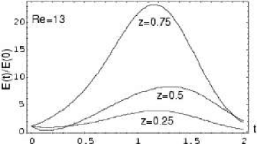
a) $\hbox{Re}=13$

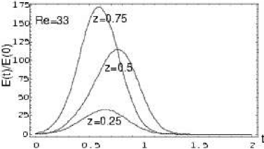
b) $\hbox{Re}=33$

Figure 6: The time dependent energy growth for $\Gamma=1,$ $\zeta=0.1~{},$ $r=0.5~{},$ $k_{r}(0)=1.0,$ $k_{z}=-1,$ $\widehat{\Psi}(0)=1.0,$ $\widehat{v}(0)=1$ for different levels of $z$, $z=0.25~{},~{}0.50~{},~{}0.75.$

We can assume that the same mechanism work also without any axial flow in the system. Consider two symmetrical counter rotating Taylor vortices in the annulus. Then we have in the annular gap a radial distribution of the axial velocity component which is oppositely directed in different parts of the annular gap. If now a small perturbation amplified the circulation in one of the vortices for a small interval of time then radial gradients of the axial velocity will show up in different parts of the gap. Therefore the degree of growth of perturbations in the continuous spectrum will be different in both parts of the gap and the faster growing perturbation can trigger an irreversible process of symmetry breaking.

5 A symmetry breaking and helicity conservation law

The classical Taylor - Couette problem with pure rotation of one or both cylinders posses $\bf Z^{2}$ and $\bf SO(3)$ symmetries. The implementation of an axial flow immediately destroyes the $\bf Z^{2}$ mirror symmetry. The axial perturbation flow amplifies in-homogeneously different intrinsic modes in the studied states as we proved in the previous section. It results in a reach variety of super critical stationary and quasi periodical states. This symmetry breaking for short cylinders can be considered as a generation of certain helicity states.

The helicity is a topological characteristic of the flow and it is the second inviscid integral invariant for the Euler equations. The helicity is defined by

$$\mathcal{H}=\mathop{\displaystyle\int}\limits_{V}\mathbf{u}\cdot\left[\nabla\times\mathbf{u}\right]dV,$$ (30)

where the vector $\Upsilon\equiv\nabla\times\mathbf{u}$ defines the vorticity of the flow. The helicity is a pseudo scalar because of

$$\mathcal{H}\left(-\mathbf{r}\right)=-\mathcal{H}\left(\mathbf{r}\right).$$

It is well known that the helicity is an important quantity in the study of dynamics and stability of complicated vortex structures and flows. The states with maximum of helicity correspond to the states with minimum of energy [36], [37], [38].

In the same way as we get the evolution equation for the energy of the system

$$\partial_{t}\mathcal{E}=\mathop{\displaystyle\oint}\limits_{S}p\cdot\mathbf{u}_{\mathbf{n}}dS-\nu\mathop{\displaystyle\int}\limits_{V}\left[\nabla\times\mathbf{u}\right]^{2}dV$$

we obtain the following evolution equation for the helicity,

$$\partial_{t}\mathcal{H}=\mathop{\displaystyle\oint}\limits_{S}\left[\nabla\times\mathbf{u}\right]_{\mathbf{n}}\left(\frac{\mathbf{u}^{2}}{2}-\frac{p}{\rho}\right)dS-\nu\mathop{\displaystyle\int}\limits_{V}\left[\nabla\times\mathbf{u}\right]\cdot\left[\nabla\times\left[\nabla\times\mathbf{u}\right]\right]dV,$$ (31)

where $\mathbf{n}$ is the unit normal vector orthogonal to the boundary surface $S.$

For the inviscid fluids the right hand side of equation (31) reduces to the first term. The helicity conserves if the normal component of the vorticity on the boundary surface disappears, $\left[\nabla\times\mathbf{u}\right]_{\mathbf{n}}=0$, or if we have a potential flow. Let $S$ include a bounded volume of an ideal fluid with $\Upsilon\neq 0$ and $\mathcal{H}\neq 0$ then the helicity will be conserved by the motion. For very small viscosity $\nu\neq 0$ the helicity is no longer conserved but it changes very slowly because of the negligibleness of the second term in (31). As a consequence, for large Reynolds numbers we can treat the helicity as an approximately conserved quantity.

In a classical Taylor-Couette system with mirror symmetric boundary conditions we expect an even number of counter-rotating vortices. The growth of anomalous modes and the phenomenon of appearing of time-dependent states can be considered as a mirror symmetry breaking process and a generation of states with a definite sign of the helicity. Let us represent the helicity in the cylindrical coordinate system and reduce the formula to the case of short cylinders. The components of the vorticity $\Upsilon$ are

$$\Upsilon_{r}=-\partial_{z}v,~{}~{}\Upsilon_{\theta}=\partial_{z}u-\partial_{r}w,~{}~{}\Upsilon_{z}=\partial_{r}v+\frac{u}{r}.$$ (32)

Using the expressions (32) we obtain for the helicity $\mathcal{H}$ in the axisymmetrical case the convenient representation

$$\mathcal{H}=4\pi\mathop{\displaystyle\iint}\limits_{S}\left(v\partial_{z}u+w\partial_{r}v+\frac{wv}{r}\right)rdrdz.$$

For a narrow annular gap with $\eta\sim 1$ and $R\gg 1$ we can approximate the formula for the helicity by

$$\mathcal{H}\cong 4\pi R\mathop{\displaystyle\iint}\limits_{S}\left(v\Upsilon_{\theta}+\frac{wv}{r}\right)drdz\approx 4\pi R\mathop{\displaystyle\iint}\limits_{S}v\Upsilon_{\theta}drdz.$$

The axial flow generates a constant stream of helicity and angular momentum through the annulus. It is an important source of the symmetry breaking in the system.

6 Numerical facilities

Major advances in computer technologies and numerical techniques have made possible to propose an alternative or at least a complementary approach to the classical and analytical techniques used in laboratory experiments. Computational Fluid Dynamics becomes part of the design process. But discontinuities or deep gradients lead to computational difficulties in the classical finite difference methods, although for the finite element methods often a suitable variational principle is not given. Therefore, we consider the finite volume methods, which are based on the integral form over a cell instead of the differential equation. Rather than a pointwise approximation at the grid points, we break the domain into grid cells and approximate the total integral over each grid cell. It is actually the cell average, which equals this integral divided by the volume of the cell.

We consider the axial symmetric case as well as the full 3D flow in the annulus. The numerical method allows to choose a so-called segregated or a coupled solver. The simulation process consists of (see e.g. [39])

• division of the domain into discrete control volumes (construction of the computational grid),

• integration of the governing equations (in axial-symmetric or in full 3D form) on the individual control volumes to construct algebraic equations for the discrete variables (velocity, pressure, temperature and other parameters),

• linearization and solution of the algebraic system to yield updated values of the variables.

Both the numerical methods of the segregated and the coupled solvers employ a similar finite volume process, but the approach used to linearize and solve the equations is different.

The FLUENT 5.5/6.0 [40] simulation and post-processing program was applied for the numerical calculation of the flow. The unsteady 2D axisymmetric or 3D version of the Navier-Stokes equations is solved as described using finite volume discretization on a structured quadrilateral grid (fig. 7).

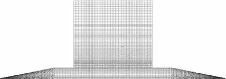
Figure 7: 2D structural grid for the annulus and the slits with 7690 quadrilateral cells.

The finite volume method has a first order upwind scheme and constant relaxation factors, while the SIMPLE procedure for the pressure-velocity coupling is applied.

The grid is generated with the help of GAMBIT program and characterized by a large difference (100 times) between boundary edges. But it was possible to save the grid structural and quadrilateral. The smallest inflow and outflow faces of the grid are divided uniformly by 20 nodes, whereas the nodes in the bigger geometry of the axial flow are a more concentrated near the boundary because some vortices can arise there if the Reynolds number is large [41]. The major volume of the annular gap is divided 50x70 nodes, uniformly in the axial direction and linear condensing in the radial direction.

As next, we set up a 2D axisymmetric model, using a rotating reference frame. The time step is selected to be $\frac{1}{80}$ of a single rotation. It helps to determine the flow motion state in the quarters of the rotation circle ($\theta=0,\pi/2,\pi,3\pi/2$). Each time step includes 30 iterations or fewer if the solution converges with the residual of order $O(10^{-5})$.

The plane of the 3D grid that corresponds to 2D axisymmetric model have to be coarser, because of the large diameter of the inner cylinder and therefore of the large number of cells in the projection on the $(r,\theta)$-plane. These are only 10 nodes on the inflow and outflow faces in the conical tapering of the slits and 25x30 in the annulus of the slits (fig. 8).

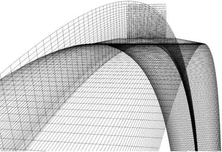
Figure 8: 3D grid with 1087040 hexahedral cells.

It results in 1087040 hexahedral cells, that is close to the limit for a computation and post-processing on a single processor in an acceptable time. Another, more complicated 3D simulation would be possible using parallel computing [42]. Such a program is used to being written with the Help of Message Passing Interface (MPI) [43] or some other specific approaches [44]. But this is the aim of further investigations and developments.

Some test simulations showed, that the 3D case is not sensitive enough to determine the very small scale instabilities correctly. Although, the results of the 3D and 2D axisymmetric simulations on the same grid are equivalent. It was verified using the same coarser grid for the 2D case or by solution of the stationary problem without instabilities. A finer grid for the 2D axisymmetric case, by contrast, does not give more substantial changes to the behavior of the unstable flow. So, the 2D axisymmetric case (fig. 7) with 7690 quadrilateral grid cells is chosen and can be considered without loss of accuracy for all computations in that geometry.

7 Pattern structure in the annulus under influence of the axial flow

In numerical experiments which simulated the flow in the annular gap as in fig. 1 and more detailed in fig. 7 both axial symmetrical and 3D cases were studied. 3D calculations had been done prepared for a large number of examples. But it became apparent that no torsion or other remarkable 3D effects arose in the system for $\mbox{Re}\leq 6000$. Therefor we used for further numerical investigations axisymmetrical case which saved a lot of time and computer capacity. As a graphical representation of the results in 3-D cases on a paper sheet does not show the interesting region in sufficient detail so that we represent only one fig. 9 which gives an impression, that the processes under investigation are indeed mostly axisymmetrical.

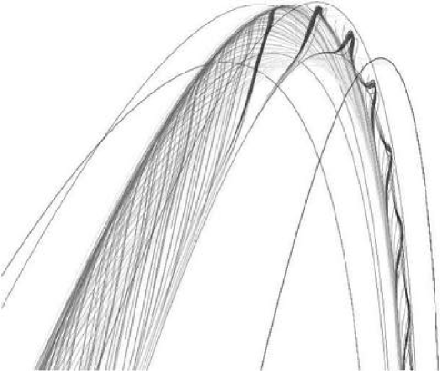
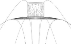
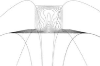
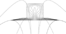
Figure 9: 3D simulation of the two symmetrical stationary vortices. Only one of the vortices is represented to avoid an overload of the left figure. The counter lines of the velocity magnitude are given in 3D case on the left and in cross sections on the right right by $\theta=0,\pi/2,\pi$, where $\nu=0.1(10^{-3}\frac{m^{2}}{s}),$ $w=0.016~{},$ $u_{max}=0.060~{},$ $\mbox{Re}=1256.0~{},$ $\mbox{Re}_{ax}=0.1~{}.$

In all investigations the inner cylinder rotates with the same azimuthal velocity $V_{0}=2\pi\omega r_{in}$ on the surface of the inner cylinder. We used this value to render other velocities dimensionless. The weak axial flow is directed on all figures from left to right. The entrance and outgoing slits in the ends of conical tapering have the radius ratio $\tilde{\eta}=0.99992.$

We found that there exist four different flow states with typical patterns in dependence on the relation between azimuthal and axial Reynolds numbers. The azimuthal Reynolds number Re is defined by $\mbox{Re}=V_{0}~{}d/\nu$ and the axial Reynolds number by $\mbox{Re}_{ax}=w_{max}~{}d/\nu.$

We studied a pure rotation and then switched on an axial flow to investigate the sensitivity of the flow patterns to small axial perturbations. The pattern structure is very sensitive to the appearance of an axial flow. We looked for very weak axial flow with $\mbox{Re}_{ax}\ll\mbox{Re}$ nevertheless the pattern structure changed immediately under the influence of the axial flow. We studied the states distribution in the regions $\mbox{Re}\in[0,12000]$ and $\mbox{Re}_{ax}\in[0,10].$ The results for the most interesting part are that for $\mbox{Re}\in[0,2500]$ and $\mbox{Re}_{ax}\in[0,1]$ and they are represented on the schematic diagram fig. 10.

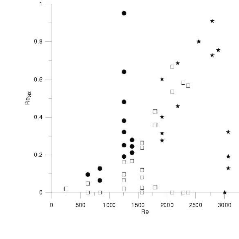
Figure 10: The pattern distribution in dependence on the azimuthal Re and axial $\mbox{Re}_{ax}$ Reynolds numbers. Two Taylors vortices in the annulus are denoted by $\square$, one stable vortex by $\bullet$, natural oscillation states of two vortices by $\bigstar.$

Let us consider the pure rotation case without any axial flow. The most probable state for a short cylinder with an aspect ratio $\Gamma\sim 1$ can be described as follows. The nearly quadratic cross section of the annulus is filled with two counter rotating stable Taylor vortices as represented on the fig. 11.

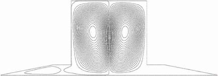
Figure 11: Two symmetrical stationary Taylor vortices which are denoted by $\square$ on the fig.10. Here is $\nu=0.8(10^{-4}\frac{m^{2}}{s}),$ $w=0~{},$ $u_{max}=0.07~{},$ $\mbox{Re}=1570,~{}\mbox{Re}_{ax}=0.$

We proved that this structure remains mirror symmetric for a large region of azimuthal Reynolds numbers, $\mbox{Re}\in[0,2500].$ The investigated states are denoted in fig.10 by boxes, $\square$, on the horizontal axes. All of them have quite the same structure - two stationary Taylor vortices in the annulus up to very high azimuthal Reynolds numbers.

An enlargement of the azimuthal Reynolds numbers leads to the second state in the annulus. For very large azimuthal Reynolds numbers $\mbox{Re}>4000$ the intrinsic instabilities give rise to perturbed states with a lot of small vortices. This flow pattern can be interpreted as a region with a fine-grained structure overlaid with a large scale structure - three Taylor-like vortices (see fig. 12).

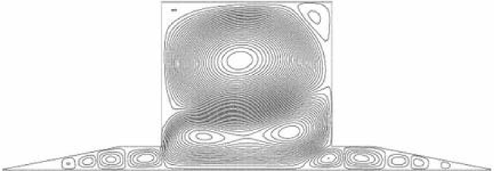
Figure 12: A lot of fine-grained structures of small vortices overlaid by large scale vortices. Here $\nu=0.1(10^{-4}\frac{m^{2}}{s}),$ $w=0~{},$ $u_{max}=0.04~{},$ $\mbox{Re}=12560~{},$ $\mbox{Re}_{ax}=0.$

Consider now the onset on an axial flow with relatively small velocity. The existence of the axial flow can be considered as a small perturbation of the base flow with pure azimuthal velocity. In the region of the azimuthal Reynolds numbers $\mbox{Re}\leq 1500$ the axial flow promoted one of the counter rotating Taylor vortices in appropriate direction. As result the annulus will be filled also for very small axial amplitudes of the axial flow with one stable vortex (see fig. 13). We see the abrupt change of the patterns structure from two stable Taylor vortices to one by switching on an axial flow. This is the third pattern structure observed in this system. It is denoted by $\bullet$ on the fig.10.

In the region on the Reynolds numbers $\mbox{Re}_{az}\sim 1500,$ $\mbox{Re}_{ax}\sim 0,4$ there exists a branch point in which three possible flow states meet. For all axial Reynolds numbers $0.05<\mbox{Re}_{ax}<4$ and $\mbox{Re}<1500$ it is the first branch for which is characterized by one stable vortex in the annulus (fig.13).

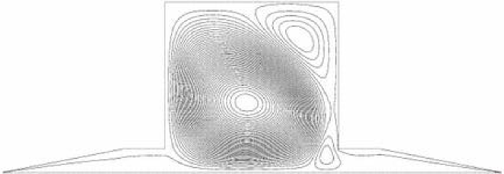
Figure 13: One large stationary vortex filling out nearly the whole annulus (denoted on the fig.10 by $\bullet$). Here $\nu=0,1(10^{-3}\frac{m^{2}}{s});$ $w=0,05~{};$ $u_{max}=0,04~{};$ $\mbox{Re}=1256~{};$ $\mbox{Re}_{ax}=0,32.$

For $1250<\mbox{Re}<2400$ and for the small axial Reynolds numbers $0<\mbox{Re}_{ax}<0.64$ a second branch with two stable Taylor vortices appears (fig.11). For $\mbox{Re}_{az}>1500$ and $0.3<\mbox{Re}_{ax}<0.9$ the third branch appears with two quasi periodically natural oscillating vortices (fig.14).

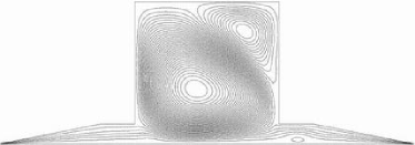
a) $t_{1}=0.402$

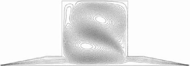
b) $t_{2}=0.427$ (minimum energy)

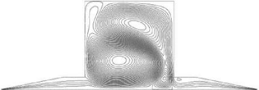
c) $t_{3}=0.478$

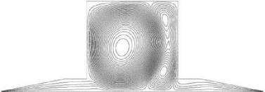
d) $t_{4}=0.490$ (maximum energy)

Figure 14: The natural quasi periodic oscillations of a two vortex state in the annulus (denoted on the fig. 10 by $\bigstar$) in four different moments of dimensionless time. Here is $\nu=0.3(10^{-4}\frac{m^{2}}{s}),$ $w=0.30~{},$ $u_{max}=0.05~{},$ $\mbox{Re}=5108~{},$ $\mbox{Re}_{ax}=6.333.$

This branch representes non stationary states. The energy and momentum of the system show also typical quasi periodical oscillations. The time dependence of the energy is given on the fig. 15. The time dependence of the angular momentum is of the same type. We rendered the energy dimensionless using its value for small Reynolds numbers, $\mbox{Re}=251.2,~{}\mbox{Re}_{ax}=0.02~{}.$ In fig. 15 we also see that maximal values for the energy are smaller in the perturbation state as in the non perturbed flow.

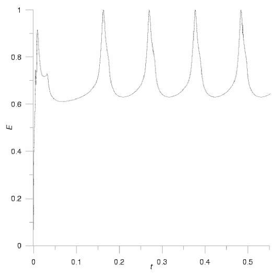
Figure 15: The time dependence of the total energy $E(t)$ for the flow by $\mbox{Re}=5108,$ $\mbox{Re}_{ax}=6,333.$

We will distinguish two different types of energy in the system - the rotation or toroidal energy, defined by

$$E_{tor}=2\pi\int v^{2}rdrdz$$

and the energy caused by axial and local radial flow in the system

$$E_{pol}=2\pi\int\left(u^{2}+w^{2}\right)rdrdz,$$

named also poloidal energy. Correspondingly with Reynolds numbers the toroidal energy is three order larger as the last one. But the intrinsic instabilities in the system lead to steady energy exchange between different motion types. This exchange we demonstrate by a parametric representation in the plane of both energies in fig. 16.

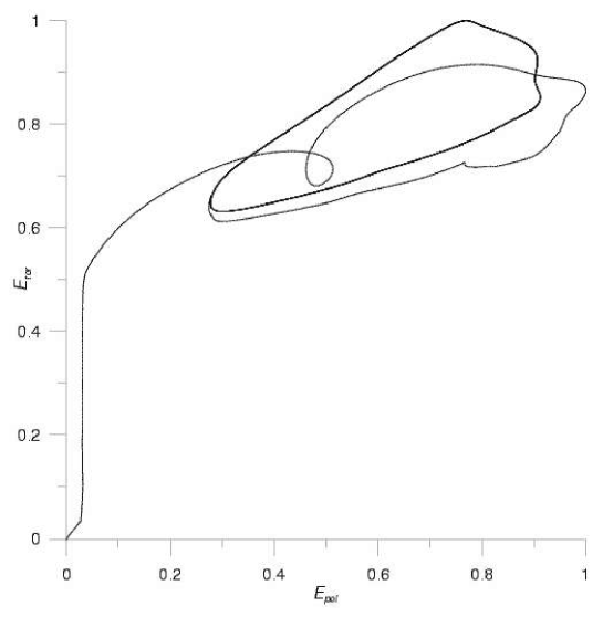
Figure 16: The parametric representation of the energy exchange between $E_{tor}$ and $E_{pol}$ in the plane of both energies by $\mbox{Re}=5108~{},$ $\mbox{Re}_{ax}=6,333$.

The flow field between differently shaped bodies of revolution were studied experimentally or theoretically rarely. The experimental work devoted to the case which is somewhat analogously to the motion in the conical slits at the caps of cylinders in our case was done by Wimmer [45]. For a rotating cylinder in a stationary cone he proved that due to the non constant gap different types of motion can coexist in the gap. By the growth of the Reynolds numbers the first vortices appear at the location of the largest gap size and are deformed, having larger axial extension. The numerical studies in our geometry confirm this statement as can be seen on the fig. 12.

8 Conclusions

The convenient asymptotic representation for the exact steady solution of the Taylor-Couette problem was found in the case of closed short cylinders $\Gamma\sim 1$ (section 3). The found approximated solution (5) will be an exact solution for infinitely large viscosity or for $Re\to 0$. For finite Reynolds numbers a flow in a thin layer along the caps of the cylinder can arise. We estimated the radial and axial components of its velocity. At first blush in the case of the strong nonlinear motion the estimation $u/V_{0}\sim R^{-1/2},$ $w/V_{0}\sim R^{-1/2}$ must hold. This follows from the comparison of the nonlinear terms in the Navier-Stokes equations. But the numerical computations for the short cylinders with $R\gg 1$ and large Reynolds numbers lead to another estimation, $u/V_{0}\sim R^{-1},$ $w/V_{0}\sim R^{-1},$ which can be obtained from the Navier-Stokes equations in the case of very large viscosity. In fig. 17 we represent the radial component of the dimensionless velocity only. For the other component the pattern distribution is quite the same.

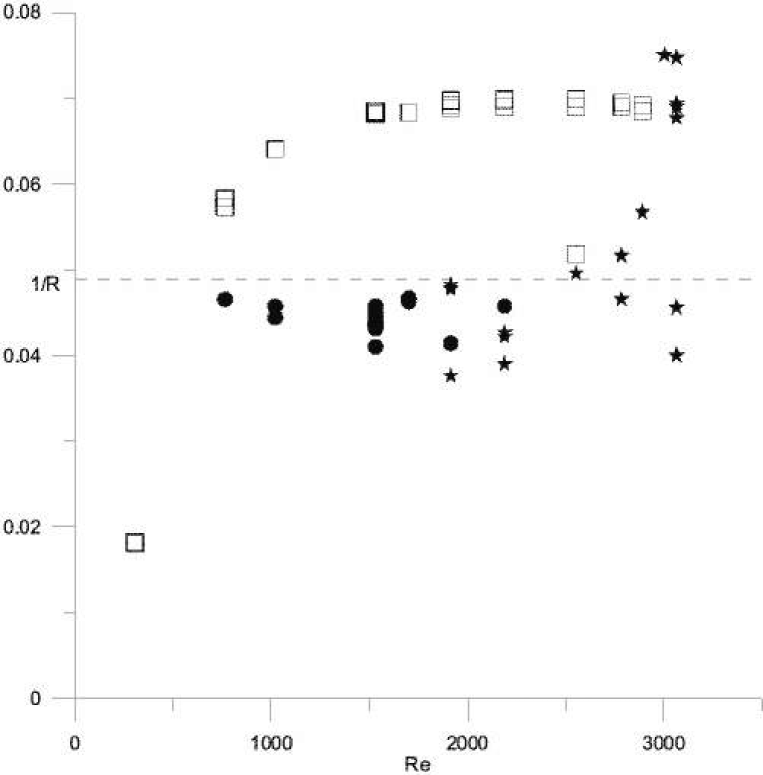
Figure 17: The distribution of the radial component of the dimensionless velocity $\max{\tilde{u}}$ in the Taylor-Coutte flow for different states in dependence on the Reynolds numbers Re and $\mbox{Re}_{ax}.$ Two Taylors vortices in the annulus are denoted by $\square$, one stable vortex by $\bullet$, natural oscillation state of two vortices by $\bigstar.$

From the estimations it follows that the azimuthal component of the velocity has the main influence on the stability of the system. Consequently, we can use for our qualitative stability analysis the found approximated solution.

The stability analysis done in section 4 showed that the inhomogeneity of the base flow in the radial direction as well as the axial flow cause a perturbation of the Rossby waves type. We proved that the $\bf Z^{2}-$symmetry breaking due to the axial flow in the Taylor-Couette flow is in the same time the helicity symmetry breaking (section 5). The states with non-zero helicity can accrue in the system (section 7). The energy oscillations in the case of the unsteady pattern with natural oscillations as in fig. 15 correspond to the helicity oscillations in the system.This can be seen from fig. 14.

The weak axial flow in an annulus between the rotating inner cylinder and the fixed outer cylinder has several important engineering applications in particular if the axial flow is directed as a thin layer along the surface of the rotating cylinder. We studied this case and proved that the axial flow stabilizes the motion and that in a system with very narrow annulus different super critical states are possible (section 7). We remark that experiments in short cylinders with an aspect ratio of $\Gamma\sim 1$ without any axial flow showed a poor variety of states [46], [47]. But for smaller aspect ratio all the states which we described in our case can be observed. This behavior of the Taylor-Couette system can be interpreted as follows. The influence of the weak axial flow along the surface of the inner cylinder can be considered as a change in the geometry, i.e., as a shortening of the axial length of the cylinder. This interpretation is supported by simple estimations.

For technical applications it is important to describe not only the velocity field but also the pressure distribution in the device. The pressure differences in the annulus coming from the vortex motion can be estimated as $R^{-1}$ of the pressure difference corresponding to the axial flow.

References

- [1] G.I. Taylor, Phil. Trans. R. Soc. London, Ser. A 223, 289 (1923).
- [2] T. Mullin and T.B. Benjamin, Nature, Lond. 288, 567 (1980).
- [3] D.G. Schaeffer, Math. Proc. Camb. Phil. Soc. 87, 307 (1980).
- [4] K. A. Cliffe and T. Mullin, J. Fluid Mech. 153, 243 (1985).
- [5] K.A. Cliffe, J.J. Kobine and T. Mullin, Proc. R. Soc. Lond. A. 439, 341 (1992).
- [6] G.P. Neitzel, C.S. Kirkconnell and L.J. Little, Phys. Fluids 7(2), 324 (1995).
- [7] A. Aitta, G. Ahlers, D.S. Cannell, Phys. Rev. Lett. 54, 673 (1985).
- [8] T. Mullin, Y. Toya and S.J. Tavener, Phys. Fluids 14(8), 2778 (2002).
- [9] J.K. Bhattacharjee, Convection and Chaos in Fluids (World Scientific, 1987).
- [10] H. Furukawa et al., Phys. Rev. E 65, 036306-1 (2002).
- [11] S. Chandrasechar, Proc. Nat. Acad. Sci., USA, 46, 141 (1960).
- [12] R.C. Di Prima, J. Fluid Mech. 9, 621 (1960).
- [13] F. Marques and J.M. Lopez, J. Fluid Mech. 348, 153 (1997).
- [14] Á. Meseguer and F. Marques, in Physics of rotating Fluids edited by Ch. Eggbers, G. Pfister (Springer, 2000) p. 119.
- [15] H.C. Hu and R.E. Kelly, Phys.Rev. E 51, 3242 (1995).
- [16] S. Chandrasekhar, Hydrodynamic and Hydromagnetic Stability (Clarendon Press, Oxford, 1961).
- [17] A.Y. Weisberg, I.G. Kevrekidis and A.J. Smits, J. Fluid Mech. 348, 141 (1997).
- [18] R. M. Lueptow, in Physics of rotating Fluids edited by Ch. Eggbers, G. Pfister (Springer, 2000) p. 137.
- [19] M.C. Wendl, Phys. Rew. E 60(5), 6192 (1999).
- [20] H. Ji, J. Goodman and A. Kageyama, arXiv:astro-ph/0103226v3 (2002).
- [21] V.A. Vladimirov et al., Matem. Met. i Vych. Exper. 13(2), 27 (2001).
- [22] L.A. Bordag, in Proceedings of 4. Tagung der Deutschen Sektion der EWM in Chemnitz, 2001, p. 3.
- [23] L.M. Milne-Thomson, Theoretical hydrodynamics (Dover Publications, New York, 1996), p. 477.
- [24] P. Goldreich and G. Schubert, Ap. J. 150, 571 (1967).
- [25] N. Lebovitz and A. Lifschitz, Astrophys. J. 40, 603 (1993).
- [26] A. Lifschitz, Phys. Lett. A 152, 3-4, 199 (1991).
- [27] A. Lifschitz and E. Hameiri, Comm. Pure and Appl. Math. XLVI, 1379 (1993).
- [28] D. G. Lominadze, G. D. Chagelishvili and R. G. Chanishvili, Soviet Astr. Lett. 14(5), 364 (1988).
- [29] K.M. Buttler and B.F. Farrel, Phys. Fluids A 4, 1627 (1992).
- [30] S.C. Reddy and D.S. Hennigson, J. Fluid Mech. 252, 209 (1993).
- [31] Á. Meseguer, Phys. Fluids 14, 1655 (2002).
- [32] H. Hristova et al., Phys.Fluids 14, 3475 (2002).
- [33] L.H. Gustavsson, Phys. Fluids 22, 1602 (1979).
- [34] G.D. Chagelishvili and O.G. Chkhetiani, JETP Lett. 62, 314 (1995).
- [35] G.D. Chagelishvili, A.D. Rogava and D.G. Tsiklauri, Phys. Rev. E 53, 6028 (1996).
- [36] H.K. Moffat and A. Tsinober, Ann. Rev. Fluid Mech. 23, 281 (1992).
- [37] O.G. Chkhetiani, Izv. Atm. Ocean. Phys. 37, 569 (2001).
- [38] O.G. Chkhetiani, V.M. Ponomarev and A.A. Khapaev, Advances in Turbulence IX (CIMNE, Barcelona, 2002) p. 224.
- [39] M. Fröhner, The Bulletin of KazNU, Math., Mech. and Inf. Issue, 4(32), 84 (2002).
- [40] FLUENT 6 Manual, Fluent Inc., 2001.
- [41] O.A. Ladyshenskaya, The Mathematical Theory of Viscous Incompressible Flow (Gordon and Breach, 2nd ed., 1969).
- [42] V. Myrnyy, Brandenburg University of Technology, Cottbus, Report M-11/2001.
- [43] MPI-2: Extensions to the Message-Passing Interface, Version 2.0, July 18, 1997.
- [44] V. Mirniy and M. Fröhner, Comp. Technology, 6(3), 32 (2001).
- [45] M. Wimmer, in Physics of rotating Fluids edited by Ch. Eggbers, G. Pfister (Springer, 2000) p. 194.
- [46] H. Furukawa, Nagoya University, Japan (unpublished)
- [47] T. Watanabe, H. Furukawa and I. Nakamura, Phys. of Fluids 14(1), 333 (2002).