How many clusters? An information theoretic perspective

Abstract

Clustering provides a common means of identifying structure in complex data, and there is renewed interest in clustering as a tool for the analysis of large data sets in many fields. A natural question is how many clusters are appropriate for the description of a given system. Traditional approaches to this problem are based either on a framework in which clusters of a particular shape are assumed as a model of the system or on a two-step procedure in which a clustering criterion determines the optimal assignments for a given number of clusters and a separate criterion measures the goodness of the classification to determine the number of clusters. In a statistical mechanics approach, clustering can be seen as a trade–off between energy– and entropy–like terms, with lower temperature driving the proliferation of clusters to provide a more detailed description of the data. For finite data sets, we expect that there is a limit to the meaningful structure that can be resolved and therefore a minimum temperature beyond which we will capture sampling noise. This suggests that correcting the clustering criterion for the bias which arises due to sampling errors will allow us to find a clustering solution at a temperature which is optimal in the sense that we capture maximal meaningful structure — without having to define an external criterion for the goodness or stability of the clustering. We show that, in a general information theoretic framework, the finite size of a data set determines an optimal temperature, and we introduce a method for finding the maximal number of clusters which can be resolved from the data in the hard clustering limit.

1 Introduction

Much of our intuition about the world around us involves the idea of clustering: many different acoustic waveforms correspond to the same syllable, many different images correspond to the same object, and so on. It is plausible that a mathematically precise notion of clustering in the space of sense data may approximate the problems solved by our brains. Clustering methods also are used in many different scientific domains as a practical tool to evaluate structure in complex data. Interest in clustering has increased recently because of new areas of application, such as data mining, image– and speech–processing and bioinformatics. In particular, many groups have used clustering methods to analyze the results of genome–wide expression experiments, hoping to discover genes with related functions as members of the same cluster; see, for example, Eisen, Spellman, Brown and Botstein (1998). A central issue in these and other applications of clustering is how many clusters provide an appropriate description of the data. The estimation of the true number of classes has been recognized as “one of the most difficult problems in cluster analysis” by Bock (1996), who gives a review of some methods that address the issue.

The goal of clustering is to group data in a meaningful way. This is achieved by optimization of a so called “clustering criterion” (an objective function), and a large variety of intuitively reasonable criteria have been used in the literature (a summary is given in Gordon, 1999). Clustering methods include agglomerative clustering procedures such as described by Ward (1963) and iterative re-allocation methods, such as the commonly used K–means algorithm (Lloyd, 1957; MacQueen, 1967), which reduces the sum of squares criterion, the average of the within cluster squared distances. More recently, algorithms with physically inspired criteria were introduced (Blatt, Wiseman and Domany 1996; Horn and Gottlieb, 2002). All these clustering methods have in common that the number of clusters has to be found by another criterion. Often, a two-step procedure is performed: The optimal partition is found for a given data set, according to the defined objective function, and then a separate criterion is applied to test the robustness of the results against noise due to finite sample size. Such procedures include the definition of an intuitively reasonable criterion for the goodness of the classification, as in Tibshirani, Walther and Hastie (2001), or performing cross–validation (Stone, 1974) and related methods in order to estimate the prediction error and to find the number of clusters that minimizes this error (e.g. Smyth, 2000). Roth, Lange, Braun and Buhmann (2002) quantify the goodness of the clustering via a resampling approach.

It would be attractive if these two steps could be combined in a single principle. In a sense this is achieved in the probabilistic mixture model approach, but at the cost of assuming that the data can be described by a mixture of $N_{c}$ multivariate distributions with some parameters that determine their shape. Now the problem of finding the number of clusters is a statistical model selection problem. There is a trading between complexity of the model and goodness of fit. One approach to model selection is to compute the total probability that models with $N_{c}$ clusters can give rise to the data, and then one finds that phase space factors associated with the integration over model parameters serve to discriminate against more complex models (Balasubramanian, 1997). This Bayesian approach has been used to determine the number of clusters (Fraley and Raftery, 2002).

From an information theoretic point of view, clustering is most fundamentally a strategy for lossy data compression: the data are partitioned into groups such that the data could be described in the most efficient way (in terms of bit cost) by appointing a representative to each group. The clustering of the data is achieved by compressing the original data into representatives, throwing away information that is not relevant to the analysis. While most classical approaches in statistics give an explicit definition of a similarity measure, in rate–distortion theory we arrive at a notion of similarity through a fidelity criterion implemented by a distortion function (Shannon 1948). The choice of the distortion function provides an implicit distinction between relevant and irrelevant information in the raw data. The notion of relevance was made explicit by Tishby, Pereira and Bialek (1999) who defined relevant information as the information which the data provide about an auxiliary variable and performed lossy compression, keeping as much relevant information as possible. This formulation, termed “Information Bottleneck method” (IB), is attractive, because the objective function follows only from information theoretical principles. In particular, this formulation does not require an explicit definition of a measure for similarity or distortion. The trade–off between the complexity of the model on one hand and the amount of relevant information it captures on the other hand is regulated by a trade-off parameter. For a given problem, the complete range of this trade–off is meaningful, and the structure of the trade–of characterizes the “clusterability” of the data. However, for a finite data set, there should be a maximal value for this trade–off after which we start to “overfit,” and this issue has not yet been addressed in the context of the IB. In related work, Buhmann and Held (2000) derived for a particular class of histogram clustering models a lower bound on the annealing temperature from a bound on the probability of a large deviation between the error made on the training data and the expected error.

In this article, we follow the intuition that if a model — which, in this context, is a (probabilistic) partition of the data set — captures information (or structure) in the data, then we should be able to quantify this structure in a way that corrects automatically for the overfitting of finite data sets. Attempts to capture only this “corrected information” will, by definition, not be sensitive to noise. Put another way, if we would separate at the outset real structure from spurious coincidences due to undersampling, then we could fit only the real structure. In the context of information estimation from finite samples there is a significant literature on the problem and we argue here that the known finite sample correction to information estimates is (in some limits) sufficient to achieve the “one-step” compression and clustering in the sense described above, leading us naturally to a principled method of finding the best clustering that is consistent with a finite data set.

We should point out that in general we are not looking for the “true” number of clusters, but rather for the maximum number of clusters which can be resolved from a finite data set. This number equals the true number only if there exists a true number of classes and if the data set is also large enough to allow us to resolve them.

2 Rate distortion theory and the Information Bottleneck Method

If data $x\in X$ are chosen from a probability distribution $P(x)$, then a complete description of a single data point requires an average code length equal to the entropy of the distribution, $S(x)=-\sum_{x}P(x)\log_{2}\left[P(x)\right]$ bits. On the other hand, if we assign points to clusters $c\in\{1,2,\cdots,N_{c}\}$, then we need at most $\log_{2}(N_{c})$ bits. For $N_{c}<<|X|$ we have $\log_{2}(N_{c})<<S(x)$, and our intuition is that many problems will allow substantial compression at little cost if we assign each $x$ to a cluster $c$ and approximate $x$ by a representative $x_{c}$.

Rate distortion theory

formalizes the cost of approximating the signal $x$ by $x_{c}$ as the expected value of some distortion function, $d(x,x_{c})$ (Shannon 1948). This distortion measure can, but need not be a metric. Lossy compression is achieved by assigning the data to clusters such that the mutual information

$$I(c;x)=\sum_{xc}P(c|x)P(x)\log_{2}\left[\frac{P(c|x)}{P(c)}\right]$$ (1)

is minimized. The minimization is constrained by fixing the expected distortion

$$\langle d(x,x_{c})\rangle=\sum_{xc}P(c|x)P(x)d(x,x_{c}).$$ (2)

This leads to the variational problem

$$\min_{P(c|x)}\left[\langle d(x,x_{c})\rangle+TI(c;x)\right].$$ (3)

The (formal) solution is a Boltzmann distribution

$$P(c|x)=\frac{P(c)}{Z(x;T)}\exp\left[-\frac{1}{T^{\prime}}d(x,x_{c})\right],$$ (4)

with the distortion playing the role of energy, and the normalization

$$Z(x,T)=\sum_{c}P(c)\exp\left[-\frac{1}{T^{\prime}}d(x,x_{c})\right]$$ (5)

playing the role of a partition function (Rose, Gurewitz and Fox, 1990). The representatives, $x_{c}$, often simply called cluster centers, are determined by the condition that all of the “forces” within each cluster balance for a test point located at the cluster center,

$$\sum_{x}P(x|c)\frac{\partial}{\partial x_{c}}d(x,x_{c})=0.$$ (6)

Recall that if the distortion measure is the squared distance, $d(x,x_{c})=(x-x_{c})^{2}$, then Eq. (6) becomes $x_{c}=\sum_{x}xP(x|c)$; the cluster center is in fact the center of mass of the points which are assigned to the cluster.

The Lagrange parameter $T$ regulates the trade–off between the detail we keep and the bit cost we are willing to pay; in analogy with statistical mechanics, $T$ often is referred to as the temperature (Rose, Gurewitz and Fox, 1990). $T$ measures the softness of the cluster membership. The deterministic limit ($T\to 0$) is the limit of hard clustering solutions. As we lower $T$ there are phase transitions among solutions with different numbers of distinct clusters, and if we follow these transitions we can trace out a curve of $\langle d\rangle$ vs. $I(c;x)$, both evaluated at the minimum. This is the rate–distortion curve and is analogous to plotting energy vs. (negative) entropy with temperature varying parametrically along the curve. Crucially, there is no optimal temperature which provides the unique best clustering, and thus there is no optimal number of clusters: more clusters always provide a more detailed description of the original data and hence allow us to achieve smaller average values of the distortion $d(x,x_{c})$, while the cost of the encoding increases.

Information Bottleneck method

The distortion function implicitly selects the features that are relevant for the compression. However, for many problems, we know explicitly what it is that we want to keep information about while compressing the data, but one can not always construct the distortion function that selects for these relevant features. In the Information Bottleneck method (Tishby, Pereira and Bialek, 1999) the relevant information in the data is defined as information about another variable, $v\in V$. Both $x$ and $v$ are random variables and we assume that we know the distribution of co-occurrences, $P(x,v)$. We wish to compress $x$ into clusters $c$, such that the relevant information, i.e. the information about $v$, is maximally preserved. This leads directly to the optimization problem

$$\max_{P(c|x)}\left[I(c;v)-TI(c;x)\right].$$ (7)

One obtains a solution similar to Eq. (4)

$$P(c|x)=\frac{P(c)}{Z(x,T)}\exp\left[-\frac{1}{T}D_{KL}[P(v|x)\|P(v|c)]\right]$$ (8)

in which the Kullback–Leibler divergence,

$$D_{KL}[P(v|x)\|P(v|c)]=\sum_{v}P(v|x)\log_{2}\left[\frac{P(v|x)}{P(v|c)}\right],$$ (9)

emerges in the place of the distortion function (Tishby, Pereira and Bialek, 1999), providing a notion of similarity between the distributions $P(v|x)$ and $P(v|c)$, where $P(v|c)$ is given by

$$P(v|c)=\frac{1}{P(c)}\sum_{x}P(v|x)P(c|x)P(x).$$ (10)

When we plot $I(c;v)$ as a function of $I(c;x)$, both evaluated at the optimum, we obtain a curve similar to the Rate Distortion Curve, the slope of which is given by the trade–off between compression and preservation of relevant information:

$$\frac{\delta I(c;v)}{\delta I(c;x)}=T.$$ (11)

3 Finite sample effects

The formulation above assumes that we know the probability distribution underlying the data, but in practice we have access only to a finite number of samples, and so there are errors in the estimation of the distribution. These random errors produce a systematic error in the computation of the cost function. The idea here is to compute the error perturbatively and subtract it from the objective function. Optimization with respect to the assignment rule is now by definition insensitive to noise and we should (for the IB) find a value for the trade–off parameter $T^{*}$ at which the relevant information is kept maximally.

The compression problem expressed in Eq. (7) gives us the right answer if we evaluate the functional (7) at the true distribution $P(x,v)$. But in practice we do not know $P(x,v)$, instead we have to use an estimate $\hat{P}(x,v)$ based on a finite data set. We use perturbation theory to compute the systematic error in the cost function that results from the uncertainty in the estimate.

We first consider the case that $P(x)$ is known and we have to estimate only the distribution $P(v|x)$. This is the case in many practical clustering problems, where $x$ is merely an index to the identity of samples, and hence $P(x)$ is constant, and the real challenge is to estimate $P(v|x)$. In section 5, we discuss the error that comes from uncertainty in $P(x)$ and also what happens when we apply this approach to rate–distortion theory.

Viewed as a functional of $P(c|x)$, $I(c;x)$ can have errors arising only from uncertainty in estimating $P(x)$. Therefore, if $P(x)$ is known, then there is no bias in $I(c;x)$. We assume for simplicity that $v$ is discrete. Let $N$ be the total number of observations of $x$ and $v$. For a given $x$, the (average) number of observations of $v$ is then $NP(x)$. We assume that the estimate $\hat{P}(v|x)$ converges to the true distribution in the limit of large data set size $N\to\infty$. However, for finite $N$, the estimated distribution will differ from the true distribution and there is a regime in which $N$ is large enough such that we can approximate (compare Treves and Panzeri, 1995)

$$\hat{P}(v|x)=P(v|x)+\delta P(v|x),$$ (12)

where we assume that $\delta P(v|x)$ is some small perturbation and its average over all possible realizations of the data is zero

$$\left\langle\delta P(v|x)\right\rangle=0.$$ (13)

Taylor expansion of $I^{\rm emp}(c;v):=I(c;v)|_{\hat{P}(v|x)}$ around $P(v|x)$ leads to a systematic error $\Delta I(c;v)$:

$$I(c;v)|_{\hat{P}(v|x)=P(v|x)+\delta P(v|x)}=I(c;v)|_{P(v|x)}+\Delta I(c;v),$$ (14)

where the error

$$\Delta I(c;v)=\sum_{n=1}^{\infty}\frac{1}{n!}\sum_{v}\sum_{x^{(1)}}\dots\sum_{x^{(n)}}\frac{\delta^{n}I(c;v)}{\prod_{k=1}^{n}\delta P(v|x^{(k)})}\left\langle\prod_{k=1}^{n}\delta P(v|x^{(k)})\right\rangle$$ (15)

with

$$\frac{\delta^{n}I(c;v)}{\prod_{k=1}^{n}\delta P(v|x^{(k)})}=(-1)^{n}(n-2)!\left[\sum_{c}\frac{\prod_{k=1}^{n}P(c|x^{(k)})}{(P(c,v))^{n-1}}-\frac{\prod_{k=1}^{n}P(x^{(k)})}{(P(v))^{n-1}}\right]$$ (16)

is given by

$$\Delta I(c;v) = \frac{1}{\ln 2}\sum_{n=2}^{\infty}\frac{(-1)^{n}}{n(n-1)}\sum_{v}\left(\sum_{c}\frac{\langle(\sum_{x}\delta P(v|x)P(c,x))^{n}\rangle}{(P(c,v))^{n-1}}\right.$$ (17)

$$\left.-\frac{\langle(\sum_{x}\delta P(v|x)P(x))^{n}\rangle}{(P(v))^{n-1}}\right),$$

Note that the terms with $n=1$ vanish, because of Eq. (13) and that the second term in the sum is constant with respect to $P(c|x)$.

Our idea is to subtract this error from the objective function (7) and to recompute the distribution that maximizes the corrected objective function.

$$\max_{P(c|x)}\left[I^{\rm emp}(c;v)-TI^{\rm emp}(c;x)-\Delta I(c;v)+\mu(x)\sum_{c}P(c|x)\right].$$ (18)

The last constraint ensures normalization, and the optimal assignment rule $P(c|x)$ is now given by

$$P(c|x) = \frac{P(c)}{Z(x,T)}\exp\left[-\frac{1}{T}\bigg{(}D_{KL}[P(v|x)\|P(v|c)]+\sum_{v}\sum_{n=2}^{\infty}\frac{(-1)^{n}}{\ln(2)}\right.$$ (19)

$$\left.\times\left[P(v|x)\frac{\langle(\delta P(v|c))^{n}\rangle}{n(P(v|c))^{n}}-\frac{\langle\delta P(v|x)(\delta P(v|c))^{n-1}\rangle}{(n-1)(P(v|c))^{n-1}}\right]\bigg{)}\right]$$

which has to be solved self consistently together with Eq. (10) and

$$\delta P(v|c):=\sum_{x}\delta P(v|x)P(x|c)$$ (20)

The error $\Delta I(c;v)$ is calculated in Eq. (17) as an asymptotic expansion and we are assuming that $N$ is large enough to ensure that $\delta P(v|x)$ is small $\forall v$. Let us thus concentrate on the term of leading order in $\delta P(v|x)$ which is given by (disregarding the term which does not depend on $P(c|x)$)

$$\left(\Delta I(c;v)\right)^{(2)}=\frac{1}{2\ln(2)N}\sum_{vc}\frac{\sum_{x}[P(c|x)]^{2}P(x|v)}{\sum_{x}P(c|x)P(x|v)},$$ (21)

where we have made use of Eq. (10) and the approximation (for counting statistics)

$$\langle\delta P(v|x)\delta P(v|x^{\prime})\rangle\simeq\delta_{xx^{\prime}}\frac{P(v|x)}{NP(x)}.$$ (22)

Can we say something about the shape of the resulting “corrected” optimal information curve by analyzing the leading order error term (Eq. 21)? This term is bounded from above by the value it assumes in the deterministic limit ($T\to 0$), in which assignments $P(c|x)$ are either 1 or 0 and thus $[P(c|x)]^{2}=P(c|x)$,

$$\left(\Delta I(c;v)\right)^{(2)}_{T\to 0}=\frac{1}{2\ln(2)}\frac{K_{v}}{N}N_{c}.$$ (23)

$K_{v}$ is the number of bins we have used to obtain our estimate $\hat{P}(v|x)$. Note that if we had adopted a continuous, rather than a discrete, treatment, then the volume of the (finite) $V$-space would arise instead of $K_{v}$. If one does not make the approximation (22) and, in addition, also keeps the terms constant in $P(c|x)$, then one obtains for the upper bound ($T\to 0$ limit) of the $n=2$ term from expression (17):

$$\frac{1}{2\ln(2)}\frac{K_{v}-1}{N}(N_{c}-1)$$ (24)

which is the leading correction to the bias as derived in (Treves and Panzeri, 1995; Eq. (2.11); term $C_{1}$). Similar to what these authors found when they computed higher order corrections we also found in numerical experiments that the leading term is a surprisingly good estimate of the total bias and we therefore feel confident to approximate the error by (21), although we can not guarantee convergence of the series in (17).

The lower bound of the leading order error (Eq. 21) is given by

$$\frac{1}{2\ln(2)}\frac{1}{N}2^{I(c;x)},$$ (25)

and hence the “corrected information curve”, which we define as

$$I^{\rm corr}(c;v):=I^{\rm emp}(c;v)-\Delta I(c;v),$$ (26)

is (to leading order) bounded from above by

$$I^{\rm corr}_{UB}(c;v)=I^{\rm emp}(c;v)-\frac{1}{2\ln(2)}\frac{1}{N}2^{I(c;x)}.$$ (27)

The slope of this upper bound is $T-2^{I(c;x)}/2N$ (using Eq. (11)), and there is a maximum at

$$T^{*}_{UB}=\frac{1}{2N}2^{I(c;x)}.$$ (28)

Figure 1: Sketch of the lower and upper bound on the corrected information curve which both have a maximum under some conditions (see Eqs. (28) and (31)), indicated by $x$-es, compared to the empirical information curve which is monotonically increasing.

If the hard clustering solution assigns equal numbers of data to each cluster, then the upper bound on the error, Eq. (23), can be rewritten as

$$\frac{1}{2\ln(2)}\frac{K_{v}}{N}2^{I(c;x)}.$$ (29)

and therefore, the lower bound on the information curve,

$$I^{\rm corr}_{LB}(c;v)=I^{\rm emp}(c;v)-\frac{1}{2\ln(2)}\frac{K_{v}}{N}2^{I(c;x)},$$ (30)

has a maximum at

$$T^{*}_{LB}=\frac{K_{v}}{2N}2^{I(c;x)}.$$ (31)

Since both upper and lower bound coincide at the endpoint of the curve, where $T\to 0$ (see sketch in Fig. 1), the actual corrected information curve must have a maximum at

$$T^{*}=\frac{\gamma}{2N}2^{I(c;x)}.$$ (32)

where $1<\gamma<K_{v}$.

In general, for deterministic assignments, the information we gain by adding another cluster saturates for large $N_{c}$, and it is reasonable to assume that this information grows sub-linearly in the number of clusters. That means that the lower bound on $I^{\rm corr}(c;v)$ has a maximum (or at least a plateau). This ensures us that $I^{\rm corr}(c;v)$ must have a maximum (or plateau), and hence that an optimal temperature exists.

In the context of the IB, asking for the number of clusters that are consistent with the uncertainty in our estimation of $P(v|x)$ makes sense only for deterministic assignments. From the above discussion, we know the leading order error term in the deterministic limit, and we define the “corrected relevant information” in the limit $T\to 0$ as:

$$I^{\rm corr}_{T\to 0}(c;v)=I^{\rm emp}_{T\to 0}(c;v)-\frac{K_{v}}{2\ln(2)N}N_{c},$$ (33)

where $I^{\rm emp}_{T\to 0}(c;v)$ is calculated by fixing the number of clusters and cooling the temperature down to obtain a hard clustering solution. While $I^{\rm emp}_{T\to 0}(c;v)$ increases monotonically with $N_{c}$, we expect $I^{\rm corr}_{T\to 0}(c;v)$ to have a maximum (or at least a plateau) at $N_{c}^{*}$, as we have argued above. $N_{c}^{*}$, is then the optimal number of clusters in the sense that using more clusters, we would not capture more meaningful structure (or in other words would “overfit” the data), and although in principle we could always use fewer clusters, this comes at the cost of keeping less relevant information $I(c;v)$.

4 Numerical results

Figure 2: Result of clustering synthetic data with $P(v|x)={\cal N}(0,\alpha(x))$; 5 possible values for $\alpha$. Displayed is the relevant information kept in the compression, computed from the empirical distribution, $I^{\rm emp}_{T\to 0}(c;v)$, which increases monotonically as a function of the number of clusters. Each curve is computed as the mean of 5 different realizations of the data with error bars of $\pm$ 1 standard deviation. $N_{v}/K_{v}$ equals 1 (diamonds), 2 (squares), 3 (down pointing triangles), 5 (stars), 10 (up pointing triangles), 15 (circles) and 50 (crosses). $N_{x}=50$ and $K_{v}=100$ for all curves. The line is drawn at the value of the information $I(x;v)$, estimated from $10^{6}$ data points.

Figure 3: Result of clustering synthetic data with $P(v|x)={\cal N}(0,\alpha(x))$; 5 possible values for $\alpha$. Displayed is the “corrected relevant information information” in the hard clustering limit, $I^{\rm corr}_{T\to 0}(c;v)$, (see Eq. 33) as a function of the number of clusters. Each curve is computed as the mean of 5 different realizations of the data with error bars of $\pm$ 1 standard deviation. $N_{v}/K_{v}$ equals 1 (diamonds), 2 (squares), 3 (down pointing triangles), 5 (stars), 10 (up pointing triangles), 15 (circles) and 50 (crosses). All individual curves (not just the means) peak at $N^{*}_{c}=5$, except for those with $N_{v}/K_{v}=1$, which peak at $N^{*}_{c}=4$. $N_{x}=50$ and $K_{v}=100$ for all curves. The line is drawn at the value of the information $I(x;v)$, estimated from $10^{6}$ data points.

Figure 4: A trivial examples of those data sets on which we found the correct number of clusters (results are summarized in Fig. 6). Here, $P(v|x)={\cal N}(\alpha(x),1)$ with 5 different values for $\alpha$, spaced $d\alpha=2$ apart. $K_{v}=100$, $N_{x}=20$, $N_{v}/K_{v}=20$.

Figure 5: One of the difficult examples of those data sets on which we found the correct number of clusters (results are summarized in Fig. 6). Here, $P(v|x)={\cal N}(\alpha(x),1)$ with 5 different values for $\alpha$, spaced $d\alpha=0.2$ apart. $K_{v}=100$, $N_{x}=20$, $N_{v}/K_{v}=20$.

Figure 6: Result of finding the correct number of clusters with our method for a synthetic data set of size $N=N_{x}N_{v}$ ($N_{x}=20$) with $P(v|x)={\cal N}(\alpha(x),1)$ and with either 2, 5 or 10 possible values for $\alpha$, spaced $d\alpha$ apart. We indicate values of $d\alpha$ and the resolution $N_{v}/K_{v}$ ($K_{v}=100$) at which the correct number of clusters is found: for 2, 5 and 10 clusters (squares); only for 2 and 5 clusters (stars); only for 2 clusters (circles). The classification error (on the training data) is 0 for all points except for the one that is labeled with $95\%$ correct.

4.1 Simple synthetic test data

We test our method for finding $N^{*}_{c}$ on data that we understand well and where we know what the answer should be. We thus created synthetic data drawn from normal distributions with zero mean and 5 different variances (for Figs. 2 and 3). We emphasize that we chose an example with Gaussian distributions not because any of our analysis makes use of Gaussian assumptions, but rather because in the Gaussian case we have a clear intuition about the similarity of different distributions and hence about the difficulty of the clustering task. This will become important later, when we make the discrimination task harder (see Fig. 6). We use $K_{v}=100$ bins to estimate $\hat{P}(v|x)$. In Figs. 2 and 3, we compare how $I_{T\to 0}^{\rm emp}(c;v)$ and $I^{\rm corr}_{T\to 0}(c;v)$ behave as a function of the number of clusters. The number of observations of $v$, given $x$, is $N_{v}=N/N_{x}$. For a large range of “resolutions” (average number of observations per bin), $N_{v}/K_{v}$, $I^{\rm corr}_{T\to 0}(c;v)$ has a maximum at $N^{*}_{c}=5$ (the true number of clusters). When we have too little data ($N_{v}/K_{v}=1$), we can resolve only 4 clusters. The curves in Figs. 2 and 3 are calculated as the mean of the curves obtained from 5 different realizations of the data, and the error bars are $\pm$ 1 standard deviation. The optimal number of clusters $N_{c}^{*}$, as determined by our method, is always the same, for each of these individual curves, so that there are no error bars on the optimal number of clusters as a function of the data set size. As $N_{v}/K_{v}$ becomes very large, $I^{\rm corr}_{T\to 0}(c;v)$ approaches $I_{T\to 0}^{\rm emp}(c;v)$, as expected.

The curves in Figs. 2 and 3 differ in the average number of examples per bin, $N_{v}/K_{v}$. The classification problem becomes harder as we see less data. However, it also becomes harder when the true distributions are more like each other. To separate the two effects, we create synthetic data drawn from Gaussian distributions with unit variance and $N_{A}$ different, equidistant means $\alpha$, which are $d\alpha$ apart. $N_{A}$ is the true number of clusters. This problem becomes intrinsically harder as $d\alpha$ becomes smaller. Examples are shown in Figs. 4 and 5. The problem becomes easier as we are allowed to look at more data, which corresponds to an increase in $N_{v}/K_{v}$. We are interested in the regime in the space spanned by $N_{v}/K_{v}$ and $d\alpha$ in which our method retrieves the correct number of clusters.

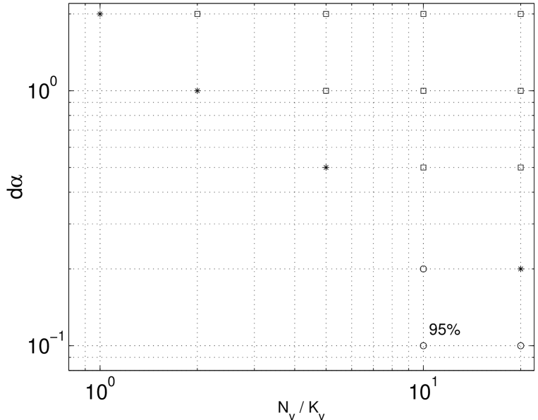
In Fig. 6, points mark those values of $d\alpha$ and $N_{v}/K_{v}$ (evaluated on the shown grid) at which we find the true number of clusters. The different shapes of the points summarize results for 2, 5 and 10 clusters. A missing point on the grid indicates a value of $d\alpha$ and $N_{v}/K_{v}$ at which we did not find the correct number of clusters. All these missing points lie in a regime which is characterized by a strong overlap of the true distributions combined with scarce data. In that regime, our method always tells us that we can resolve fewer clusters than the true number of clusters. For small sample sizes, the correct number of clusters is resolved only if the clusters are well separated, but as we accumulate more data, we can recover the correct number of classes for more and more overlapping clusters. To illustrate the performance of the method, we show in Fig. 5 the distribution $P(x,v)$ in which $\alpha(x)$ has 5 different values which occur with equal probability, $P(\alpha(x))=1/5$ and which differ by $d\alpha=0.2$. For this separation, our method still retrieves 5 as the optimal number of clusters when we have $N_{v}=2000$ observations per example $x$.

Our method detects when only one cluster is present, a case in which many methods fail (Gordon, 1999). We verified this for data drawn from one Gaussian distribution and for data drawn from the uniform distribution.

Figure 7: 20000 data points drawn from a radial distribution, according to $P(r)={\cal N}(1,0.2)$, with $x=rcos(\phi)$, $v=rsin(\phi)$, $P(\phi)=1/2\pi$. Displayed is the estimated probability distribution (normalized histogram with 50 bins along each axis).

Figure 8: $I^{\rm emp}_{T\to 0}(c;v)$ as a function of the number of clusters, averaged over 7 different realizations of the data. Error bars are $\pm$ 1 standard deviation. The information $I(x;v)$ calculated from 100000 data points is 0.58 bits (line). Data set size $N$ is: 100 (diamonds), 300 (squares), 1000 (down pointing triangles), 3000 (stars), 10000 (up pointing triangles), 30000 (circles), 100000 (crosses).

Figure 9: $I^{\rm corr}_{T\to 0}(c;v)$ as a function of the number of clusters, averaged over 7 different realizations of the data. Error bars are $\pm$ 1 standard deviation. The information $I(x;v)$ calculated from 100000 data points is 0.58 bits (line). Data set size $N$ is: 100 (diamonds), 300 (squares), 1000 (down pointing triangles), 3000 (stars), 10000 (up pointing triangles), 30000 (circles), 100000 (crosses).

Figure 10: Optimal number of clusters, $N_{c}^{*}$, as found by the suggested method, as a function of the data set size $N$. The middle curve (crosses) represents the average over 7 different realizations of the data, points on the upper/lower curve $\pm$ 1 standard deviation. Line at 25.

4.2 Synthetic test data that explicitly violates mixture model assumptions

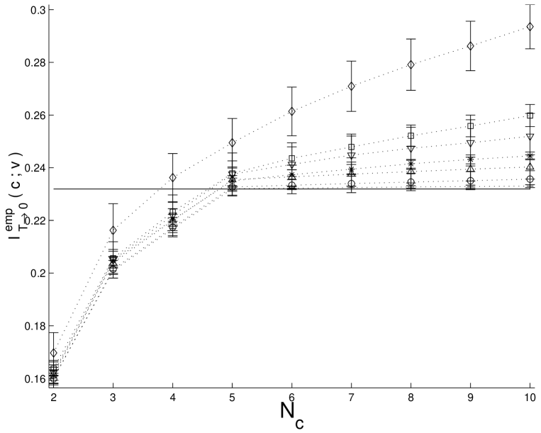
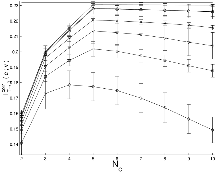
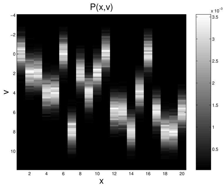
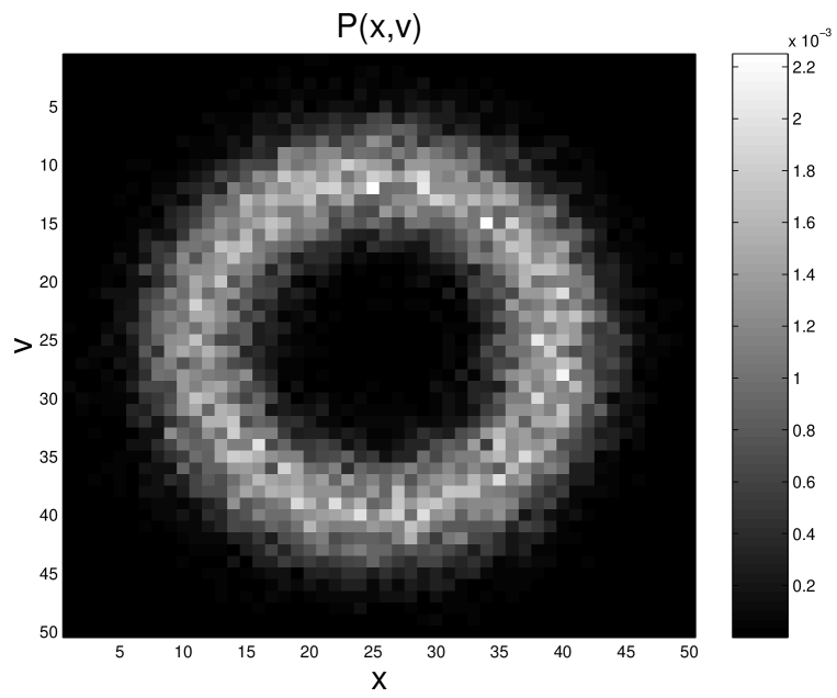
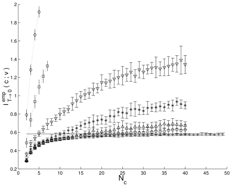
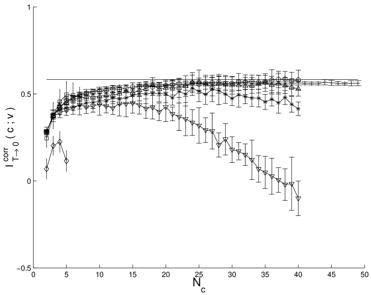
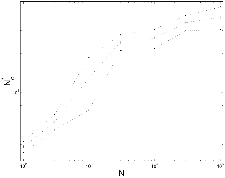
We consider data drawn from a radial normal distribution, according to $P(r)={\cal N}(1,0.2)$, with $x=rcos(\phi)$, $v=rsin(\phi)$, and $P(\phi)=1/2\pi$, as shown in Fig. 7. The empirical information curves (Fig. 8) and corrected information curves (Fig. 9) are computed as the mean of 7 different realizations of the data for different sample sizes. The corrected curves peak at $N_{c}^{*}$, which is shown as a function of $N$ in Fig. 10. For less than a few thousand samples, the optimal number of clusters goes roughly as $N_{c}^{*}\propto N^{2/3}$, but there is a saturation around $N_{c}^{*}\approx 25$. This number corresponds to half of the number of x-bins (and therefore half of the number of “objects” we are trying to cluster) which makes sense given the symmetry of the problem.

5 Uncertainty in $P(x)$

In the most general case, $x$ can be a continuous variable drawn from an unknown distribution $P(x)$. We then have to estimate the full distribution $P(x,v)$ and if we want to follow the same treatment as above, we have to assume that our estimate approximates the true distribution

$$\hat{P}(v,x)=P(v,x)+\delta P(v,x),$$ (34)

where $\delta P(v,x)$ is some small perturbation and its average over all possible realizations of the data is zero

$$\left\langle\delta P(v,x)\right\rangle=0.$$ (35)

Now, this estimate induces an error not only in $I^{\rm emp}(c;v)$, but also in $I^{\rm emp}(c;x)$. Taylor expansion of these two terms gives

$$\Delta I(c;v) = \frac{1}{\ln(2)}\sum_{vc}\sum_{n=2}^{\infty}\frac{(-1)^{n}}{n(n-1)}\left(\frac{1}{(P(v,c))^{n-1}}-\frac{1}{(P(c))^{n-1}}\right)$$ (36)

$$\times\left\langle\left(\sum_{x}P(c|x)\delta P(x,v)\right)^{n}\right\rangle-\Lambda(P(v))$$

$$\Lambda(P(v)) = \frac{1}{\ln(2)}\sum_{v}\sum_{n=2}^{\infty}\frac{(-1)^{n}}{n(n-1)}\frac{1}{(P(v))^{n-1}}\left\langle\left(\sum_{x}\delta P(x,v)\right)^{n}\right\rangle$$ (37)

$$\Delta I(c;x) = -\frac{1}{\ln(2)}\sum_{vc}\sum_{n=2}^{\infty}\frac{(-1)^{n}}{n(n-1)}\frac{1}{(P(c))^{n-1}}$$ (38)

$$\times\left\langle\left(\sum_{x}P(c|x)\delta P(x,v)\right)^{n}\right\rangle$$

This results in a correction to the objective function ($F^{\rm corrected}=F^{\rm emp}-\Delta F$), given by:

$$\Delta F = \frac{1}{\ln(2)}\sum_{vc}\sum_{n=2}^{\infty}\frac{(-1)^{n}}{n(n-1)}\frac{1}{(P(c))^{n-1}}\left(\frac{1}{(P(v|c))^{n-1}}+T-1\right)$$

$$\times\left\langle\left(\sum_{x}P(c|x)\delta P(x,v)\right)^{n}\right\rangle-\Lambda(P(v)),$$

where $\Lambda(P(v))$ is constant in $P(c|x)$ and therefore not important. At critical temperature $T=1$, the error due to uncertainty in $P(x)$ made in calculating $I^{\rm emp}(c;v)$ cancels that made in computing $I^{\rm emp}(c;x)$. For small $T$, the largest contribution to the error is given by the first term in the sum of Eq. (5), since $1/(P(v|c))^{n}\geq 1$, $\forall\{n,v,c\}$. Therefore, the procedure that we have suggested for finding the optimal number of clusters in the deterministic limit ($T\to 0$) remains unchanged, even if $P(x)$ is unknown. Let us consider, as before, the leading order term of the error (using the approximation in Eq. (22))

$$\left(\Delta F\right)^{(2)}=\frac{1}{2N\ln(2)}\sum_{cv}\frac{1}{p(c)}\left(\frac{1}{p(v|c)}+T-1\right)\sum_{x}(P(c|x))^{2}P(x,v).$$ (40)

In the $T\to 0$ limit this term becomes $N_{c}(K_{v}-1)/2N\ln(2)$, and we find,

$$I_{T\to 0}^{\rm corr}(c;v)=I_{T\to 0}^{\rm emp}(c;v)-\frac{K_{v}-1}{2\ln(2)N}N_{c},$$ (41)

which is insignificantly different from Eq. (33) in the regime $K_{v}>>1$.

Only for very large temperatures $T>>1$ (i.e. at the onset of the annealing process) could the error that results from uncertainty in $P(x)$ make a significant difference.

The corrected objective function is now given by

$$F^{\rm corr}=I^{\rm emp}(c;v)-TI^{\rm emp}(c;x)-\Delta F-\mu(x)\sum_{c}P(c|x),$$ (42)

and the optimal assignment rule is given by

$$P(c|x) = \frac{P(c)}{Z(x,T)}\exp\bigg{[}-\frac{1}{T}\bigg{(}D_{KL}\left[P(v|x)\|P(v|c)\right]$$ (43)

$$+\frac{1}{\ln(2)P(x)}\sum_{v}\sum_{n=2}^{\infty}(-1)^{n}\bigg{[}\frac{1}{n(P(c))^{n}}\left(\frac{1}{(P(v|c))^{n}}+T-1\right)$$

$$\times\left\langle(\delta P(v,c))^{n}\right\rangle-\frac{1}{(n-1)(P(c))^{n-1}}\left(\frac{1}{(P(v|c))^{n-1}}+T-1\right)$$

$$\times\left\langle\delta P(x,v)(\delta P(v,c))^{n-1}\right\rangle\bigg{]}\bigg{)}\bigg{]},$$

which has to be solved self consistently together with Eq. (10) and

$$\delta P(v,c):=\sum_{x}\delta P(v,x)P(c|x)$$ (44)

Rate–distortion theory.

Let us assume that we estimate the distribution $P(x)$ by $\hat{P}(x)=P(x)+\delta P(x)$, with $\langle\delta P(x)\rangle=0$, as before. While there is no systematic error in the computation of $\langle d\rangle$, this uncertainty in $P(x)$ does produce a systematic under estimation of the information cost $I(c;x)$:

$$\Delta I(c;x)=-\frac{1}{\ln(2)}\sum_{n=2}^{\infty}\frac{(-1)^{n}}{n(n-1)}\sum_{c}\frac{\left\langle\left(\sum_{x}P(c|x)\delta P(x)\right)^{n}\right\rangle}{(P(c))^{n-1}}$$ (45)

When we correct the cost functional for this error (with $\lambda=1/T$),

$$F^{\rm corr}:=I(c;x)+\lambda\langle d(x,x_{c})\rangle-\Delta I(c;x)+\mu(x)\sum_{c}P(c|x),$$ (46)

we obtain for the optimal assignment rule (with $\lambda^{\prime}=\lambda\ln(2)$),

$$P(c|x) =\frac{P(c)}{Z(x,\lambda)}\exp \left[-\lambda^{\prime}d(x,x_{c})+\sum_{c}\sum_{n=2}^{\infty}\left(\frac{\left\langle\left(\sum_{x}P(c|x)\delta P(x)\right)^{n}\right\rangle}{n\left(P(c)\right)^{n}}\right.\right.$$ (47)

$$-\left.\left.\frac{1}{P(x)}\frac{\left\langle\delta P(x)\left(\sum_{x}P(c|x)\delta P(x)\right)^{n-1}\right\rangle}{(n-1)\left(P(c)\right)^{n-1}}\right)\right].$$

Let us consider the leading order term of the error made in calculating the information cost,

$$\left(\Delta I(c;x)\right)^{(2)}=-\frac{1}{2\ln(2)N}\sum_{c}\frac{\langle\sum_{x}\left(P(c|x)\delta P(x)\right)^{2}\rangle}{P(c)}.$$ (48)

For counting statistics, we can approximate, as before,

$$\left(\Delta I(c;x)\right)^{(2)}\approx-\frac{1}{2\ln(2)N}\sum_{c}\frac{\sum_{x}\left(P(c|x)\right)^{2}P(x)}{P(c)}.$$ (49)

The information cost is therefore underestimated by at least $2^{I(c;x)}/2$ bits. The corrected rate–distortion curve with

$$I^{\rm corr}(c;x):=I(c;x)-\Delta I(c;x)$$ (50)

is then bounded from below by

$$I^{\rm corr}_{LB}(c;x)=I(c;x)+\frac{1}{2\ln(2)N}2^{I(c;x)}$$ (51)

and this bound has a rescaled slope given by

$$\tilde{\lambda}=\lambda^{\prime}\left(1-\frac{1}{2N}2^{I(c;x)}\right)$$ (52)

but no extremum. Since there is no optimal trade–off, it is not possible to use the same arguments as we have used before to determine an optimal number of clusters in the hard clustering limit. To do this, we have to carry the results obtained from the treatment of the finite sample size effects in the IB over to rate–distortion theory. This is possible, with insights we have gained in Still, Bialek and Bottou (2004) about how to use the IB for data that are given with some measure of distance (or distortion).

6 Summary

Clustering, as a form of lossy data compression, is a trade–off between the quality and complexity of representations. In general, a data set (or clustering problem) is characterized by the whole structure of this trade–off — the rate–distortion curve or the information curve in the IB method — which quantifies our intuition that some data are more clusterable than others. In this sense there is never a single “best” clustering of the data, just a family of solutions evolving as a function of temperature.

As we solve the clustering problem at lower temperatures, we find solutions that reveal more and more detailed structure and hence have more distinct clusters. If we have only finite data sets, however, we expect that there is an end to the meaningful structure that can be resolved — at some point separating clusters into smaller groups just corresponds to fitting the sampling noise. The traditional approach to this issue is to solve the clustering problem in full, and then to test for significance or validity of the results by some additional statistical criteria. What we have presented in this work is, we believe, a new approach: Because clustering is formulated as an optimization problem, we can try to take account of the sampling errors and biases directly in the objective functional. In particular, for the Information Bottleneck method all terms in the objective functional are mutual informations, and there is a large literature on the systematic biases in information estimation. There is a perturbative regime in which these biases have a universal form and can be corrected. Applying these corrections, we find that at fixed sample size the trade–off between complexity and quality really does have an endpoint beyond which lowering the temperature or increasing the number of clusters does not resolve more relevant information. We have seen numerically that in model problems this strategy is sufficient to set the maximum number of resolvable clusters at the correct value.

Acknowledgments

We thank N. Tishby for helpful comments on an earlier draft. S. Still wishes to thank M. Berciu and L. Bottou for helpful discussions and acknowledges support from the German Research Foundation (DFG), grant no. Sti197.

References

• V. Balasubramanian, Statistical Inference, Occam’s Razor, and Statistical Mechanics on the Space of Probability Distributions. Neural Comp. 9 (1997) 349.

• M. Blatt, S. Wiseman and E. Domany, Superparamagnetic Clustering of Data. Phys. Rev. Lett. 76 (1996) 3251-3254, cond-mat/9702072

• H.-H. Bock, Probability Models and Hypotheses Testing in Partitioning Cluster Analysis. In Clustering and Classification Eds.: P. Arabie, L.J. Hubert and G. De Soete (1996) World Scientific, pp. 378-453.

• J. M. Buhmann and M. Held, Model Selection in Clustering by Uniform Convergence Bounds. In Adv. Neural Inf. Proc. Sys. (NIPS) 12 Eds.: S. A. Solla, T. K. Leen and K.-R. Müller (2000) MIT Press, Cambridge, MA

• M. Eisen, P. T. Spellman, P. O. Brown and D. Botstein, Cluster analysis and display of genome-wide expression patterns. Proc. Nat. Acad. Sci. (USA) 95 (1998) 14863.

• C. Fraley and A. Raftery, Model-based clustering, discriminant analysis, and density estimation. J. Am. Stat. Assoc. 97 (2002) 611.

• A. D. Gordon, Classification, (1999) Chapmann and Hall/CRC Press, London

• P. Hall and E. J. Hannan, On stochastic complexity and nonparametric density estimation. Biometrika 75 (1988) No. 4, pp.705-714.

• D. Horn and A. Gottlieb, Algorithm for Data Clustering in Pattern Recognition Problems Based on Quantum Mechanics. Phys. Rev. Lett. 88 (2002) 018702, extended version: physics/0107063

• S. Lloyd, Least squares quantization in PCM. Technical Report (1957) Bell Laboratories. Also in: IEEE Trans. Inf. Th., vol. IT-28 (1982) 129.

• J. MacQueen, Some methods for classification and analysis of multivariate observations. In Proc. 5th Berkeley Symp. Math. Statistics and Probability Eds.: L.M.L Cam and J. Neyman (1967) University of California Press, pp. 281-297 (Vol. I)

• K. Rose, E. Gurewitz and G. C. Fox, Statistical Mechanics and Phase Transitions in Clustering. Phys. Rev. Lett. 65 (1990) 945.

• V. Roth, T. Lange, M. Braun and J. M. Buhmann, A Resampling Approach to Cluster Validation. In Proceedings in Computational Statistics: 15th Symposium, Berlin , Germany 2002 (COMPSTAT2002), Eds.: W. Härdle, Bernd Rönz (2002) Physica-Verlag, Heidelberg, pp.123-128.

• C. E. Shannon, A mathematical theory of communication. Bell System Tech. J. 27, (1948). 379–423, 623–656. See also: C. Shannon and W. Weaver, The Mathematical Theory of Communication (1963) University of Illinois Press

• P. Smyth, Model selection for probabilistic clustering using cross-validated likelihood. Statistics and Computing 10 (2000) 63.

• S. Still, W. Bialek and L. Bottou, Geometric Clustering using the Information Bottleneck method. Advances In Neural Information Processing Systems 16 Eds.: S. Thrun, L. Saul, and B. Schölkopf (2004) MIT Press, Cambridge, MA.

• M. Stone, Cross-validatory choice and assessment of statistical predictions. J. R. Stat. Soc. 36 (1974) 111.

• R. Tibshirani, G. Walther and T. Hastie, Estimating the number of clusters in a dataset via the Gap statistic. J. R. Stat. Soc. B 63 (2001) 411.

• N. Tishby, F. Pereira and W. Bialek, The information bottleneck method. In Proc. 37th Annual Allerton Conf. Eds.: B. Hajek and R. S. Sreenivas (1999) University of Illinois, physics/0004057

• A. Treves and S. Panzeri, The upward bias in measures of information derived from limited data samples. Neural Comp. 7 (1995) 399.

• J. H. Ward, Hierarchical groupings to optimize an objective function. J. Am. Stat. Assoc. 58 (1963) 236.