Energy mechanism of charges analyzed in real current environment
Reuven Ianconescu
26 Rothenstreich Str., Tel-Aviv, Israel
r_iancon@excite.com
L .P. Horwitz
School of Physics and Astronomy, Raymond and Beverly Sackler,
Faculty of Exact Sciences, Tel Aviv University,
Ramat Aviv 69978, Israel
larry@post.tau.ac.il
We analyze in this work the energy transfer process of accelerated
charges, the mass fluctuations accompanying this process, and their
inertial properties. Based on a previous work, we use here the dipole
antenna, which is a very convenient framework for such analysis, for
analyzing those characteristics.
We show that the radiation process can be viewed by two energy
transfer processes: one from the energy source to the charges and the second
from the charges into the surrounding space. Those processes, not being in
phase, result in mass fluctuations. The same principle is true during
absorption. We show that in a transient period between absorption and
radiation the dipole antenna gains mass according to the amount of absorbed
energy and loses this mass as radiated energy. We rigorously prove that the
gain of mass, resulting from electrical interaction has inertial
properties in the sense of Newton’s third low. We arrive to this
result by modeling the reacting spacetime region by an electric
dipole.
Key words: radiation resistance, self force, energy transfer, charges.
PACS: 41.60.-m, 41.20.-q, 84.40.Ba
1. INTRODUCTION
The common belief that an accelerating charge always radiates energy is reviewed. There are two Lienard-Wiechert potentials: one retarded and one advanced. For reasons of causality, the advanced solution is usually disregarded. It is considered as a field which “knows” the future motion of a charged particle. But another way of interpreting the advanced field is to define it as the field which establishes the future motion of the particles.
Let us imagine a stationary charged particle, and some remote source of radiation, distributed spatially in such a way as to create radiation of the same pattern as a dipole antenna, but propagating inwards towards the particle. May such a field correspond exactly to the advanced field of one charged particle? The answer here is no, because the advanced field contains the Coulomb component, and there is no way to create a Coulomb field from a far distributed source (because of the Gauss law). In other words it is obvious that the advanced field cannot create the state of a single charged particle.
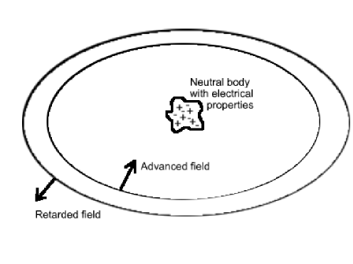
But if we modify the above question: may such a field correspond exactly to the advanced field of a neutral distribution of charged particles? Such a distribution is Coulomb free, and therefore the answer here is yes. The best example of such a charge distribution is an antenna. Also a single electric dipole is a good approximation to such a charge distribution. And one may state that as long as the advanced field does not interact with the above charge distribution, there is no charge (because the interaction domain is neutral). The charge becomes evident during the interaction. In this case one may state that the advanced field creates the charges. Or, in other words the advanced field converges into the future space-time domain of the charges, and creates a new body defined by the charge distribution.
It is to be mentioned that considering the interaction region as totally neutral before the interaction occurs, does not reduce the generality of the problem, because we assume the universe is neutral, and hence every charge in nature has its opposite sign counterpart. Therefore every space-time region is neutral on a sufficiently large scale. In this work we consider the interaction region to be large enough to validate the neutral system assumption; alternatively, we may restrict ourselves to systems which are locally neutral.
Where does this energy go now? If this charge distribution antenna is connected to a resistor which equals the radiation resistance of the antenna (i.e. impedance-matched), the energy transforms into heat. If the antenna is in open circuit (or shorted), the energy is radiated back into the space, on the same radiation pattern, and we will show that during the period of interaction, the antenna gains inertial mass.
This energy radiated back into the surrounding space will be represented by the retarded field, i.e. the field caused by the past charged distribution, or caused by the past (electric) existence of the body, as shown in Figure 1.
So interpreting the advanced field as an incoming energy (according to the definition of the advanced Green’s function), and symmetrically the retarded field as an outgoing energy, and knowing that both fields depend on acceleration of charges, we may generalize the statement: “an accelerating charge always radiates energy”, to: accelerating charges always radiate or absorb energy. There are two novel ideas here. One is that acceleration may indicate radiation or absorption, i.e. interaction [1], and the second is that the interaction is a collective process during which charges accumulate energy from a source and release it to a destination, and not a single charge process by which a charge “radiates its energy away”.
The known expression for the radiated power of a charged particle is . For an on-shell particle, , therefore we have the identity . So the radiated power could be expressed as . Interactions always occur slightly off-shell [2] (example: if gravitation acts like acceleration, and under the equivalence principle gravitation changes the metric, acceleration should change the metric too), so during interactions the above on-shell identity () is not exactly satisfied.
One should therefore ask which one of the two expressions represents better the radiated power ? It comes out that radiated power cannot come from the charge itself, but from some source which boosted the charge (for example a charge passing through a static electric field will accelerate, by absorbing energy from the static field, and radiate it). We will show that while is responsible for the radiation, is responsible for the energy absorption from the source, and therefore the difference between them, , represents a transient mass fluctuation.
In Section 2 we present the main results of a previous work [3], in which we analyzed the physical meaning of the self force on a charge which is part of a radiating antenna. This self force was associated with the radiation resistance of the antenna. We will bring here also some new insights and interpretations.
In Section 3 we develop the self force on a charge which is part of a radiating or absorbing antenna. We will show here that while for the radiating case, the self force generates the radiation resistance, for the impedance-matched absorbing antenna the self force is responsible for the dissipated heat.
In Section 4 we present an open circuit antenna which receives a short energy pulse from the surrounding space and radiates it back. We show that during the interaction process, the antenna gains an addition of inertial mass which equals the received energy, and loses the additional mass after radiation.
In Section 5, we explicitly show how the above mass gain has inertial
properties.
2. SELF-FORCE ACTING AS RADIATION RESISTANCE
In a previous work [3] it has been shown that the so called “self force” is responsible for the radiation resistance of an antenna. We will bring in this section, for convenience, the main results of this work, plus some new interpretations.
The following problem, of a driven short dipole antenna of length , was formulated:
Given the fact that any time dependence can be expanded in a Fourier series of functions, we consider the harmonic time dependence, as shown in Figure 2. But the results we obtained for the fields are correct in general, and we use the harmonic dependence only when calculating the radiation resistance, which is indeed frequency dependent.
The dependence of the current is disregarded, the antenna being short.
It comes out therefore that the motion parameters (velocity, acceleration, and its derivative) of the charges have the form
| (1) |
By describing the conductor as a continuum of single charges, as in Figure 3, we examined the forces on the “test charge” B, as a result of a disturbance produced on charge A. This disturbance is expressed in terms of the motion parameters of charge A, i.e. the acceleration and its derivative.
The motion parameters are connected to the current via:
| (2) |
where is the electrical current and is the free charge density of the conductor. The discretization of the continuum into single charges is done by defining discrete charges of value at distance so that , as in Figure 3. Furthermore, the velocity of the charges in a conductor is extremely small (order of magnitude of ).
The result obtained for the disturbing field was (3):
| (3) |
It was shown [3] that the term in (3), being in opposite phase with the velocity of the charge, and the velocity being in phase with the current, is the only term in (3) representing the damping force for the source.
The damping force is
| (4) |
therefore the “self” work (or power) is
| (5) |
| (6) |
The magnitude represents the short dipole antenna length, and the wavelength .
Another way to look at is to define the “self” voltage as an integral on the “self” field :
| (7) |
and obtain as .
It is remarkable that the “self force”, calculated with the micro parameters, shows up in macro to have the meaning of a damping power which is responsible for the radiation resistance.
Up to here, we have given the main results of [3]. Let us now compare between the “self power”, which was shown to act as damping power, and the radiated power.
The power radiated by a (low velocity) charge is
| (8) |
The “self power” equals identically , so this is the power the current source pumps. Therefore, it represents the power generated by the current source, and pumped into the charges. On the other hand, the radiated power represents the power which the charges release into space.
Using (1), we see that and . We remark that the energy over an entire cycle of both powers is identical, so the energy is conserved in average, however there is a phase shift between them, suggesting that the charges accumulate energy, before radiating it into space.
| (9) |
where is easily shown to be equal to and is also the peak value of or (which are equal up to a phase).
It is generally assumed that mass shell remains fixed classically, and varies only in quantum mechanics; we disagree because the on shell condition always imposes constraints which might contradict reality. For example it imposes the constraint for any force in Newton’s law.
Therefore, interacting particles should not be completely on-shell [2], so we will interpret (9) by considering the charges slightly off-shell:
| (10) |
The reason for choosing the off-shell factor will become clear later, and it is to be mentioned that , as we stated already. Taking the derivative of the left side with respect to the proper time, and the derivative of the right side with respect to the time (supposing time and proper time are almost equivalent), we obtain:
| (11) |
where . By taking again the derivative, we obtain:
| (12) |
The relativistic expression of the self force ), multiplied by the particle’s velocity , results in identically on-shell, but in our case it gives:
| (13) |
We remark that in (9). The mass of a radiating antenna is therefore:
| (14) |
where is the integration constant and represents the interaction-free mass of the antenna, and represents the average radiated power.
It is obvious that the free mass is preserved in average, because we dealt here with a stationary case of harmonic signal for which energy is pumped into the charges and almost immediately radiated into the space.
The mass variation will be further examined in Section 4, for a short
excitation pulse.
3. ANTENNA ABSORBING ADVANCED FIELDS AND RADIATING RETARDED FIELDS
As we saw, the “self” retarded field of a charge, acting on its neighbor, generates for a radiating antenna a “self” voltage which, divided by the current results in the radiation resistance.
It is therefore natural to analyze the “self” advanced field of a charge, acting on its neighbor, for an absorbing antenna.
We therefore derive the the retarded and advance field on charge B, by the motion of the disturbed charge A.
The near field of a charge is expressed by [3]
| (15) |
where is the null vector from charge A to charge B, given by
| (16) |
The null vector condition is imposed by
| (17) |
hence
| (18) |
Expressing , knowing that , we may express as
| (19) |
The position of charge A may be expanded in series of
| (20) |
where , and are the position, acceleration and its derivative of charge A at , respectively, and we chose the reference frame so that the velocity is at .
| (21) |
where . The the null vector condition may be rewritten as follows
| (22) |
This may be solved in first approximation by . By setting the first approximation solution into (22), we obtain the retarded/advanced solution for
| (23) |
| (24) |
We may expand :
| (25) |
and obtain
| (26) |
Using (23), we expand , and in powers of , keeping terms up to :
| (27) |
| (28) |
| (29) |
Setting those values into (26), we obtain
| (30) |
here we replace by , which is the average distance between charges, as described in Figure 3.
| (31) |
Dealing with harmonic excitation, , and . Having smaller by 11 orders of magnitude than light velocity, is completely negligible relative to , for any frequency, and we obtain:
| (32) |
where the upper sign refers to retarded and the lower sign refers to advanced (compare with (3)).
The first term is always cancelled by the force of the “other” neighbor, it therefore can be completely ignored.
The third term is identical to what is considered to be the field which creates the retarded/advanced self-force of a charge, but here it was derived as the force on a charge, due to a disturbance on a neighboring charge. As we shall see, it is the only term which responsible for the radiation/absorption resistance (which is a local phenomenon on the world line).
We will call the last 2 terms of (32) , obtaining
| (33) |
The potential difference on a wire segment of length , resulting from , will be denoted as the “self” tension (or “self” voltage) and is calculated by
| (34) |
The magnitude is according to the discretization of the charge distribution, so we get from (33) and (34)
| (35) |
According to (2)
| (36) |
Dealing with harmonic excitation (see (1)) is like multiplication by (up to a phase).
| (37) |
The power radiated/absorbed by the segment is and given by
| (38) |
According to (1), . The constant ratio between and means that the current is “in phase” with its second derivative, and therefore the first part of in (38), integrated over time, represents radiated or absorbed energy. However, the multiplication of by has the form of and therefore the second part of represents a reactive power, which results in zero energy after integrating on an integer number of time cycles. The reactive power represents power which is returned to the source each time cycle. We are therefore interested in the first term of in (38).
We therefore obtain
| (39) |
(compare with (5)). The radiation/absorption resistance is obtained by or by the first part of in (34) divided by the current :
| (40) |
The radiation resistance is the same as in (6), and the absorption resistance is obviously its negative counterpart.
This is because a negative resistance through which a current flows is completely equivalent to a current source with an internal resistance . If we connect a load resistance of the same value to this current source, as in the right side of Figure 4, we get an impedance-matched absorbing antenna.
We proved here that the advanced field behaves like an absorbed field, and knowing that the Poynting vector associated with the advanced field is of the same size and opposite direction as the Poynting vector associated with the retarded field, we may clearly state that the absorbed power is
| (41) |
(compare with (8)).
From here on we may follow the same arguments from Section 2, from (8) to (14), and get the analogous results for an absorbing antenna, which are basically the results for a radiating antenna, with sign changed.
The power accumulated by the charges is
| (42) |
where is the peak value of or (which are equal up to a phase).
The mass of an absorbing antenna comes out to be
| (43) |
where is the interaction-free mass of the antenna, and represents the average absorbed power.
We see that the mass of an antenna is expressed via the integral on
the self force of its off-shell charges
, and the difference between the
radiating and absorbing cases is the sign. This sign difference is
associated with the fact that .
4. THE TRANSIENT FROM ABSORPTION TO RADIATION
We saw in the Sections 2 and 3 that the mass of an antenna radiating or absorbing an harmonic signal, oscillates harmonically at twice the radiating/absorbing frequency.
The harmonic signal has no local time properties, hence the above results cannot describe transients between emission and absorption.
We analyze here the case of an antenna of whose discretized charges have a constant acceleration for a short period of time . As we saw in Section 3, acceleration can indicate radiation or absorption, so we will consider the case for which in the first half of the acceleration duration (time from to ) there is absorption, and in the second half of the acceleration duration (time from to ) there is radiation.
The retarded/advance field due to a discretized charge in Figure 3 at the location of its neighbor is given by the last 2 terms in (32):
| (44) |
where the upper sign refers to retarded and the lower sign refers to advanced, and the first term in (32) is always cancelled by the force of the “other” neighbor.
The force on the neighbor charge will therefore be
| (45) |
where the lower sign refers to the absorption time interval ( to ), and the upper sign to the radiation time interval ( to ).
Here we defined the mass as minus the product of two neighboring charges over the distance between them. We shall see in Section 5 that such a configuration of a pair of charges has inertial properties of magnitude , hence when the charges are opposite in sign they behave like a positive mass, and vice versa.
Actually our model in Figure 3 considered equal (free) charges in a conductor, but we know that for each negative charge there is a positive counterpart, so we will consider for now in (45) as positive: .
According to (45), the dynamic mass is
| (46) |
We want to investigate the behavior of the dynamic mass change during the interaction, i.e. from time to . For , an absorption occurs, therefore the lower sign has to be used, and for , the upper sign has to be used.
A fixed acceleration means that if we go to the rest frame of the particle by Lorentz transformation at any proper time, and measure the acceleration in this frame, we always get the same result . Under this definition, is not identically . A fixed accelerated motion, in the direction may be parametrized in the following way:
| (47) | |||
| (48) | |||
| (49) |
where the components of the 4-vectors are .
This low order approximation maintains the mass shell constraint [2] , neglecting the correction noted in (10). But we shall see below, that this off-shell term will reappear.
In the framework of a conductor, we showed [3] that the velocity of the charges is of order of magnitude of , hence , so we have to use the limit of (47)-(49) around the apex, up to first order in (note that for , )
| (50) | |||
| (51) | |||
| (52) |
We divide now the component of , by the component of , to set it in (46), and get for the absorption period
| (53) |
and for the radiation period
| (54) |
During the absorption period, there is a mass gain of , and using , the mass gain is
| (55) |
and similarly, during the radiation period there is a mass loss, resulting in a negative mass gain:
| (56) |
We recognize in the expressions for the gain and lost of mass, the
absorbed and radiated energies, respectively, exhibiting energy
conservation.
5. INERTIAL BEHAVIOR OF CHARGES
The analysis, done up to this point, was based on the discretization of an antenna into equally spaced charges, attributing to a given charge micro parameters (, , ), connected to the antenna macro parameters, like and . We eventually considered for a short antenna, the distance between 2 charges , as a representative length of the antenna.
With the aid of this model, we have succeeded to prove that the retarded field behaves like a radiated field and the advanced field behaves like an absorbed field. We have shown that during radiation or absorption the mass of the antenna (defined as ), oscillates at twice the frequency.
When the antenna absorbs an energy pulse, the mass increases according to the absorbed energy, and during the re-radiation of the pulse, the mass decreases.
In the current section we wish to make a rigorous analysis to show that an electrically reacting spacetime region has inertial properties. We model this reacting spacetime region by an ideal electric dipole. We define here an ideal dipole, as two equal and opposite charges at a distance , so that for any possible acceleration of this system:
| (57) |
Note that is unitless, therefore condition (57) is well defined. It means that the distance between the charges is short enough for the largest possible acceleration that may be considered.
The formulation is based on Figure 5
In Figure 5 the charges appear as but we will be eventually interested in the case of . The charges are bound, and they move together on the axis.
We calculate the field on , caused by , in an inertial system in which is at rest.
The most general expression for the electromagnetic tensor of a moving charge is given by [4]
| (58) |
where refer to retarded and advanced respectively, , being the observation point and the particle’s world line. Expression (58) is calculated at which satisfies
| (59) |
Equation (59) has always two solutions for , the earlier corresponds to retarded and the later to advanced.
The values we shall set in (58) for a constant acceleration along the axis are
| (60) |
| (61) |
because the observation point is defined as the location of when it is at rest, i.e. at the apex of the hyperbola.
| (62) |
therefore
| (63) |
We obtain for the tensor
| (64) |
The tensor is the transpose of (64), so we obtain for
| (65) |
The scalar is
| (66) |
| (67) |
So we obtain the EM field tensor
| (68) |
and by using the equality we may simplify it to
| (69) |
Now we have to find which satisfies (59)
| (70) |
By using the equality we find that , and is found by solving (70) for
| (71) |
We remark that both retarded and advanced fields are identical for our case, because by setting (71) in (69), the signs cancel.
We obtain, from these results, the EM tensor field
| (72) |
We calculate now the 4-force on the charge . The velocity of charge is zero in our reference frame, as we defined before, so the 4-velocity is . The force on is then
| (73) |
Similarly if we calculate the force on the charge , caused by , we just have to reverse the axis, so we obtain
| (74) |
The force on the whole system is therefore
| (75) |
The only component of the force is in the direction of the acceleration
| (76) |
For an ideal dipole, according to (57), , and the force is proportional to the acceleration:
| (77) |
We defined here , and dealing with , comes out and is a positive quantity.
We remark that the configuration defined in Figure 5 cannot radiate, and we see that it behaves like a simple constant mass. That is why we did not have to bother whether to use retarded or advanced field, and both fields gave the same result (see remark after (71)). Another way of understanding this is by the fact that for the world line described in (60).
Now, does this mass represent inertia? Yes, because if some obstacle is put in the way of the accelerating body, this obstacle will “feel” the force , exactly as it will feel it for any non-electrical body of mass M. The obstacle will be hit by an accelerating body, and will absorb the force , hence the dipole has inertial properties of magnitude .
However, the problem as exposed above, describing an accelerating dipole is not completely defined, because we must say what caused it to accelerate. But we can look at it from a different point of view: suppose we observed a static dipole from a frame accelerating in the direction.
Any mass that we observe from an accelerating system will appear
to us as being driven by an imaginary force (we call it imaginary
aposteriori, knowing we are not in an inertial system, but we observe it
as a real force). In other words, if the dipole would not have EM
mass, we would not have observed the force. And again, we can measure
this mass by dividing the imaginary force , in our case by the
acceleration , and obtain .
6. DISCUSSION
The purpose of this work was to clarify the energy transfer process between charged bodies and the world surrounding them.
We showed here that the “self” retarded field of a charge, acting on its neighbor, generates for a radiating antenna a “self” voltage which, divided by the current results in the radiation resistance (), and similarly the “self” advanced field of a charge, acting on its neighbor, generates for an absorbing matched antenna a “self” voltage which, divided by the current results in minus the radiation resistance (), i.e. acts like current source with internal resistance .
We showed also that the radiation process of an antenna consists of two energy transfer processes: energy transfer from the current source to the charges (expressed by ), and energy transfer from the charges to the surrounding space (expressed by ). Those two processes are not in phase, and therefore the mass of the antenna fluctuates at twice the radiation frequency.
Similarly, the absorption process of an antenna consists of two energy transfer processes: energy transfer from the surrounding space to the charges, and energy transfer from the charges to the resistive absorber. In this case the mass of the antenna fluctuates at twice the absorption frequency, too.
In a transient period between absorption and radiation, we found out that during absorption the mass of the antenna increases by the amount of energy absorbed, and during the radiation period the mass of the antenna decreases by the amount of energy radiated.
Another interesting conclusion is that bound charges, always appearing in nature as dipoles, are a manifestation of energy (inertia).
In a philosophical way, one may say that charge itself can be considered as a manifestation of the interaction process. This may be understood in the following way. From a macroscopic point of view, an antenna is completely neutral in the absence of interaction. The charges of course exist all the time, but they annihilate each other. During the interaction, the charges form dipoles, and appear as mass fluctuations.
References
- [1] J.A. Wheeler and R. P. Feynman, “Interaction with the Absorber as the Mechanism of Radiation”, Rev. Mod. Physics Vol. 17, 157 (1945)
- [2] O. Oron and L.P. Horwitz, “Classical Radiation Reaction Off-Shell Corrections to the Covariant Lorentz Force”, Phys. Lett. A, Vol. 280, pp. 265-270 (2001).
- [3] Reuven Ianconescu and L. P. Horwitz, “Self-Force of a Charge in a Real Current”, Foundations of Physics Letters, Vol. 15, Number 6, pp. 551-559 (December 2002).
- [4] F. Rohrlich, Classical Charged Particles (Addison-Wesley, Reading, MA 1990).