Incompressible Couette Flow

Abstract

This project work report provides a full solution of simplified Navier Stokes equations for The Incompressible Couette Problem. The well known analytical solution to the problem of incompressible couette is compared with a numerical solution. In that paper, I will provide a full solution with simple C code instead of MatLab or Fortran codes, which are known. For discrete problem formulation, implicit Crank-Nicolson method was used. Finally, the system of equation (tridiagonal) is solved with both Thomas and simple Gauss Method. Results of both methods are compared.

1 Introduction

Main problem is shown in figure (1). There is viscous flow between two parallel plates. Upper plate is moving in x direction with constans velocity $(U=U_{e})$. Lower one is not moving $(U=0)$. We are looking for a solution to describe velocity vector field in the model (between two plates).

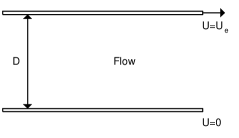
Figure 1: Schematic representation of Couette Flow Problem

2 Fundamental Equations

Most of incompressible fluid mechanics (dynamics) problems are described by simple Navier-Stokes equation for incompressible fluid velocity, which can be written with a form:

$$\frac{\partial\vec{u}}{\partial t}=(-\vec{u}\vec{\nabla})\vec{u}-\vec{\nabla}\varphi+\upsilon\vec{\nabla}^{2}\vec{u}+\vec{g},$$ (1)

where $\varphi$ is defined is defined as the relation of pressure to density:

$$\varphi=\frac{p}{\rho}$$ (2)

and $\upsilon$ is a kinematics viscosity of the fluid.

We will also use a continuity equation, which can be written as follows :

$$D=\vec{\nabla}\cdot\vec{v}=0$$ (3)

Of course, in a case of couette incompressible flow we will use several simplifications of (1).

3 Mathematical Formulation of the Couette Problem

Incompressible couette problem is not needed to solve full Navier-Stokes equations. There is no external force, so first simplification of (1) will be:

$$\frac{\partial\vec{u}}{\partial t}=(-\vec{u}\vec{\nabla})\vec{u}-\vec{\nabla}\varphi+\upsilon\vec{\nabla}^{2}\vec{u},$$ (4)

In [1] there can be found easy proof that in couette problem there are no pressure gradients, which means that:

$$\vec{\nabla}\varphi=0,$$ (5)

We will ignore a convection effects so, equation (4) can be written with a form:

$$\frac{\partial\vec{u}}{\partial t}=\upsilon\vec{\nabla}^{2}\vec{u}$$ (6)

Now we have simple differential equation for velocity vector field. That equation is a vector type and can be simplified even more. Let us write continuity equation (3) in differential form. Let $\vec{u}=(u,v)$, then continuity equation can be expanded as follows:

$$\frac{\partial u}{\partial x}+\frac{\partial v}{\partial y}=0$$ (7)

We know that there is no $u$ velocity component gradient along x axis (symmetry of the problem), so:

$$\frac{\partial u}{\partial x}=0$$ (8)

Evaluation of Taylor series at points $y=0$ and $y=D$ gives us a proof that only one possible and physically correct value for y component of velocity $\vec{u}$ is:

$$v=0$$ (9)

Because of (9) equation (6) can be written as follows:

$$\frac{\partial u}{\partial t}=\upsilon\frac{\partial^{2}u}{\partial y^{2}}$$ (10)

Our problem is now simplified to mathematical problem of solving equations like (10). That is now a governing problem of incompressible couette flow analysis.

3.1 Analytical soulution

Analytical solution for velocity profile of steady flow, without time-changes (steady state) can be found very easily in an equation:

$$\upsilon\frac{\partial^{2}u}{\partial y^{2}}=0$$ (11)

And without any changes of viscosity $\upsilon$ it can be written in form:

$$\frac{\partial^{2}u}{\partial y^{2}}=0$$ (12)

After simple two times integration of equation (12) we have analytical solution function of (12):

$$u=c_{1}\cdot y+c_{2}$$ (13)

where $c_{1}$ and $c_{2}$ are integration constans.

3.2 Boundary Conditions for The Analytical Solution

Simple boundary conditions are provided in that problem. We know that:

$$u=\left\{\begin{array}[]{ll}0&\textrm{y=0}\\ u_{e}&\textrm{y=D}\end{array}\right.$$ (14)

Simple applying it to our solution (13) gives a more specified one, where $c_{1}=\frac{u_{e}}{D}$ and $c_{2}=0$:

$$u=\frac{u_{e}}{D}\cdot y$$ (15)

It means, that a relationship between $u$ and $y$ is linear. A Better idea to write that with mathematical expression is:

$$\frac{u}{y}=\frac{u_{e}}{D}$$ (16)

Where $\frac{u_{e}}{D}$ is a constans for the problem (initial $u$ velocity vs size of the model).

4 Numerical Solution

4.1 Non-dimensional Form

Let us define some new non-dimensional variables:

$$u=\left\{\begin{array}[]{lll}u^{{}^{\prime}}&=&\frac{u}{u_{e}}\\ y^{{}^{\prime}}&=&\frac{y}{D}\\ t^{{}^{\prime}}&=&\frac{t}{D/u_{e}}\end{array}\right.$$ (17)

Now let us place these variables into equation (10) and we have now a non-dimensional equation written as follows:

$$\rho\frac{\partial u/u_{e}}{(t\cdot u_{e})/D}\left(\frac{u^{2}_{e}}{D}\right)=\upsilon\frac{\partial^{2}(u/u_{e})}{\partial(y/D)^{2}}\left(\frac{u_{e}}{D^{2}}\right)$$ (18)

Now we replace all the variables to nondimensional, like defined in (17):

$$\rho\frac{\partial u^{{}^{\prime}}}{\partial t^{{}^{\prime}}}\left(\frac{u^{2}_{e}}{D}\right)=\upsilon\frac{\partial^{2}u^{{}^{\prime}}}{\partial y^{{}^{\prime}2}}\left(\frac{u_{e}}{D^{2}}\right)$$ (19)

Now we will remove all ${}^{{}^{\prime}}$ chars from that equation (only for simplification of notation), and the equation becomes to:

$$\frac{\partial u}{\partial t}=\left(\frac{\upsilon}{D\rho u_{e}}\right)\frac{\partial^{2}u}{\partial y^{2}}$$ (20)

In that equation Reynold’s number $Re$ appears, and is defined as:

$$Re=\frac{D\rho u_{e}}{\upsilon}$$ (21)

Where $Re$ is Reynold’s number that depends on $D$ height of couette model. Finally, the last form of the equation for the couette problem can be written as follows:

$$\frac{\partial u}{\partial t}=\left(\frac{1}{Re}\right)\frac{\partial^{2}u}{\partial y^{2}}$$ (22)

We will try to formulate numerical solution of the equation (22).

4.2 Finite - Difference Representation

In our solution of equation (22) we will use Crank-Nicolson technique, so discrete representation of that equation can be written as:

$$u_{j}^{n+1}=u_{j}^{n}+\frac{\Delta t}{2(\Delta y)^{2}Re}(u_{j+1}^{n+1}+u_{j+1}^{n}-2u_{j}^{n+1}+u_{j-1}^{n+1}+u_{j-1}^{n})$$ (23)

Simple grouping of all terms which are placed in time step (n+1) on the left side and rest of them - on right side, gives us an equation which can be written as:

$$Au^{n+1}_{j-1}+Bu^{n+1}_{j}+Au^{n+1}_{j+1}=K_{j}$$ (24)

Where $K_{j}$ is known and depends only on values $u$ at $n$ time step:

$$K_{j}=\left(1-\frac{\Delta t}{(\Delta y)^{2}Re}\right)u^{n}_{j}+\frac{\Delta t}{2(\Delta y)^{2}Re}(u^{n}_{j+1}+u^{n}_{j-1})$$ (25)

Constans $A$ and $B$ are defined as follows:

$$A=-\frac{\Delta t}{2(\Delta y)^{2}Re}$$ (26)

$$B=1+\frac{\Delta t}{(\Delta y)^{2}Re}$$ (27)

4.3 Crank - Nicolson Implicit scheme

For numerical solution we will use one-dimensional grid points $(1,\ldots,N+1)$ where we will keep calculated $u$ velocities. That means $u$ has values from the range $(u_{1},u_{2},\ldots,u_{N+1})$. We know (from fixed boundary conditions), that: $u_{1}=0$ and $u_{N+1}=0$. Simple analysis of the equation (24) gives us a system of equations, which can be described by matrix equation:

$$\mathbf{A}\cdot\vec{X}=\vec{Y}$$ (28)

Where $\mathbf{A}$ is tridiagonal $[N-1]\cdot[N-1]$ matrix of constant $A$ and $B$ values:

$$\mathbf{A}=\left[\begin{array}[]{llllll}B&A&&&&\\ A&B&A&&&\\ &&\ldots&&&\\ &&&\ldots&&\\ &&&A&B&A\\ &&&&A&B\\ \end{array}\right]$$ (29)

$\vec{X}$ vector is a vector of $u$ values:

$$\vec{X}=[u_{1},u_{2},\ldots,u_{N+1}]$$ (30)

$\vec{Y}$ vector is a vector of constans $K_{j}$ values:

$$\vec{Y}=[K_{1},\ldots,K_{N+1}]$$ (31)

5 Solving The System of Linear Equations

Now the problem comes to solving the matrix - vector equation (28). There are a lot of numerical methods for that, and we will try to choose two of them: Thomas and Gauss method. Both are very similar, and I will start with a description of my implementation with the simple Gauss method.

5.1 Gauss Method

Choice of the Gauss method for solving system of linear equations is the easiest way. This simple algorithm is well known, and we can do it very easily by hand on the paper. However, for big matrices (big $N$ value) a computer program will provide us with a fast and precise solution. A very important thing is that time spent on writing (or implementing, if Gauss procedure was written before) is very short, because of its simplicity.

I used a Gauss procedure with partial choice of a/the general element. That is a well known technique for taking the first element from a column of a matrix for better numerical accuracy.

The whole Gauss procedure of solving a system of equations contains three steps. First, we are look- ing for the general element.

After that, when a general element is in the first row (we make an exchange of rows) we make some simple calculations (for every value in every row and column of the matrix) for the simplified matrix to be diagonal (instead of a tridiagonal one which we have at the beginning). That is all, because after diagonalization I implement a simple procedure (from the end row to the start row of the matrix) which calculates the whole vector $\vec{X}$. There are my values of $u_{i}$ velocity in all the model.

5.2 Thomas Method

Thomas’ method, described in [1] is simplified version of Gauss method, created especially for tridiagonal matrices. There is one disadvantage of Gauss method which disappears when Thomas’ method is implemented. Gauss method is rather slow, and lot of computational time is lost, because of special type of matrix. Tridiagonal matrices contain a lot of free (zero) values. In the Gauss method these values joins the calculation, what is useless.

Thomas’ simplification for tridiagonal matrices is to get only values from non-zero tridiagonal part of matrix. Simply applying a Thomas’ equations for our governing matrix equation (28) gives us:

$$d_{i}^{{}^{\prime}}=B-\frac{A^{2}}{d_{i-1}^{{}^{\prime}}}$$ (32)

$$u_{i}^{{}^{\prime}}=u_{i}-\frac{u_{i}^{{}^{\prime}}A}{d_{i-1}^{{}^{\prime}}}$$ (33)

We know that exact value of $u_{M}$ is defined as follows:

$$u_{M}=\frac{u^{{}^{\prime}}_{M}}{B}$$ (34)

Now solution of the system of equations will be rather easy. We will use recursion like that:

$$u_{i-1}=\frac{u^{{}^{\prime}}_{i-1}-A\cdot u_{i}}{B}$$ (35)

That easy recursion provides us a solution for the linear system of equations.

6 Results

Main results are provided as plots of the function:

$$\frac{y}{D}=f\left(\frac{u}{u_{e}}\right)$$ (36)

In figure (2) there is drawn an analytical solution to the problem of couette flow. That is linear function, and we expect that after a several time steps of numerical procedure we will have the same configuration of velocity field.

Figure 2: Analytical exact solution.

6.1 Different Time Steps

In figure (3) there are results of velocity $u$ calculation for several different time steps. Analytical solution is also drawn there.

Figure 3: Results for different time steps of numerical calculations.

As we can see in the figure (3) - the solution is going to be same as analytical one. Beginning state (known from boundary conditions) is changing and relaxing.

6.2 Results for Different Reynolds Numbers

In the figure (4) there is plot of numerical calculations for different Reynold’s numbers. For example Reynold’s number depends on i.e. viscosity of the fluid, size of couette model. As it is shown on the plot there is strong relationship between the speed of the velocity field changes and Reynold’s number. In a couple of words: when Reynolds number increases - frequency of changes also increases.

Figure 4: Calculation for same time ($t=2500$) and different Reynold’s numbers.

6.3 Results for Different Grid Density

In figure (5) there is an example of calculations of velocity field for different grid density ($N$ number). We see that there is also strong correlation between grid density, and speed of changes on the grid. Also, very interesting case $N=10$ shows, that for low density of the grid changes are very fast, and not accurate.

Figure 5: Calculation for same time ($t=2500$), same Reynold’s numbers (Re=5000) and different grid density ($N$ number).

6.4 Conclusion

Solving of Incompressible Couette Problem can be good way to check numerical method, because of existing analytical solution. In that report there were presented two methods of solving system of equations: Gauss and Thomas’ method. System of equations was taken from Crank-Nicolson Implicit scheme. Well known linear relationships were observed.

7 APPENDIX A

#include <stdlib.h>
#include <stdio.h>
#include <math.h>

#define N (40)
#define NN (N+1)

void Zamien(double *a, double *b) {
    double c;
    c=*a;   *a=*b;  *b=c;
}

void WypiszMacierz(double A[NN][NN], int n) {
    int i,j;

    for(j=1;j<n;j++)
    {
        for(i=1;i<n;i++)            // show matrix
        {
            printf("%2.4f   ",A[i][j]);
        }
        printf("\n");
    }
}

void Gauss(double A[NN][NN], double *b, double *x, int n) {
    int i,j,k;
    double m;

// Gauss Elimination

    for(i=0;i<n;i++)
    {
        // Step #1: Change governing element

        m=fabs(A[i][i]);
        k=i;

        for(j=i+1;j<n;j++)
        if(fabs(A[i][j])>m)
        {
            m=fabs(A[i][j]);
            k=j;
        }
        if(k!=i)
        for(j=0;j<n;j++)
        {
            Zamien(&A[j][i],&A[j][k]);
            Zamien(&b[i+1],&b[k+1]);
        }

        // Step #2: make it triangle
        for(j=i+1;j<n;j++)
        {
            m = A[i][j]/A[i][i];

            for(k=i;k<n;k++)
                A[k][j] = A[k][j] - m*A[k][i];

            b[j+1] = b[j+1] - m*b[i+1];
        }
    }
// Step#3: Solve now
    for(i=n-1;i>=1;i--)
    {
        for(j=i+1;j<n;j++)
            b[i+1] = b[i+1]-A[j][i]*x[j+1];
        x[i+1] = b[i+1]/A[i][i];
    }
}

int main(void)
{
    double U[N*2+2]={0},A[N*2+2]={0},B[N*2+2]={0},C[N*2+2]={0},D[N*2+2]={0},Y[N*2+2]={0};
// initialization
    double OneOverN = 1.0/(double)N;
    double Re=5000;                     // Reynolds number
    double EE=1.0;                      // dt parameter
    double t=0;
    double dt=EE*Re*OneOverN*2;         // delta time
    double AA=-0.5*EE;
    double BB=1.0+EE;
    int KKEND=1122;
    int KKMOD=1;
    int KK;                             // for a loop
    int i,j,k;                          // for loops too
    int M;                              // temporary needed variable
    double GMatrix[NN][NN]={0};             // for Gauss Elimination
    double test;
    Y[1]=0; // init

// apply boundary conditions for Couette Problem

    U[1]=0.0;
    U[NN]=1.0;

// initial conditions (zero as values of vertical velocity inside of the couette model)

    for(j=2;j<=N;j++)
        U[j]=0.0;

    A[1]=B[1]=C[1]=D[1]=1.0;

    for(KK=1;KK<=KKEND;KK++)
    {
        for(j=2;j<=N;j++)
        {
            Y[j]=Y[j-1]+OneOverN;
            A[j]=AA;
            if(j==N)
                A[j]=0.0;
            D[j]=BB;
            B[j]=AA;
            if(j==2)
                B[j]=0.0;
            C[j]=(1.0-EE)*U[j]+0.5*EE*(U[j+1]+U[j-1]);
            if(j==N)
                C[j]=C[j]-AA*U[NN];
        }

// Gauss
// C[]       -   free
// A[]B[]D[] -   for matrix calculation
// U[]       -   X

// calculate matrix for Gauss Elimination

        GMatrix[0][0]=D[1];
        GMatrix[1][0]=A[1];

        for(i=1;i<N-1;i++)
        {
            GMatrix[i-1][i]=B[i+1];     // GMatrix[1][2]=B[2]
            GMatrix[i][i]=D[i+1];       // GMatrix[2][2]=D[2]
            GMatrix[i+1][i]=A[i+1];     // GMatrix[3][2]=A[2]
        }

        GMatrix[N-2][N-1]=B[N];
        GMatrix[N-1][N-1]=D[N];

        Gauss(GMatrix,C,U,N);           // Gauss solving function

        Y[1]=0.0;
        Y[NN]=Y[N]+OneOverN;

        t=t+dt;                         // time increment
        test=KK % KKMOD;

       if(test < 0.01)                  // print the results
        {
            printf("KK,TIME\n");        // info 1
            printf("%d,%f\n",KK,t);

            printf(",J,Y[J],U[j]\n");   // info 2
            for(j=1;j<=NN;j++)
                printf("%d , %f, %f\n",j,U[j],Y[j]);
                printf("\n \n \n \n");      // for nice view of several datas
        }
     }

    return (1);
}

8 APPENDIX B

#include <stdlib.h>
#include <stdio.h>

#define N (50)
#define NN (N+1)

int main(void)
{
    double U[N*2+2],A[N*2+2],B[N*2+2],C[N*2+2],D[N*2+2],Y[N*2+2];
// initialization

    double OneOverN = 1.0/(double)N;
    double Re=7000;                     // Reynolds number
    double EE=1.0;                      // dt parameter
    double t=0;
    double dt=EE*Re*OneOverN*2;         // delta time
    double AA=-0.5*EE;
    double BB=1.0+EE;
    int KKEND=122;
    int KKMOD=1;
    int KK;                             // for a loop
    int j,k;                            // for loops too
    int M;                              // temporary needed variable

    double test;
    Y[1]=0; // init

// apply boundary conditions for Couette Problem
    U[1]=0.0;
    U[NN]=1.0;

// initial conditions (zero as values of vertical velocity inside of the couette model)
    for(j=2;j<=N;j++)
        U[j]=0.0;
    A[1]=B[1]=C[1]=D[1]=1.0;

    printf("dt=%f,    Re=%f,   N=%d \n",dt,Re, N);

    for(KK=1;KK<=KKEND;KK++)
    {
        for(j=2;j<=N;j++)
        {
            Y[j]=Y[j-1]+OneOverN;
            A[j]=AA;
            if(j==N)
                A[j]=0.0;

            D[j]=BB;
            B[j]=AA;

            if(j==2)
                B[j]=0.0;
            C[j]=(1.0-EE)*U[j]+0.5*EE*(U[j+1]+U[j-1]);

            if(j==N)
                C[j]=C[j]-AA*U[NN];
        }

        // upper bidiagonal form
        for(j=3;j<=N;j++)
        {
            D[j]=D[j]-B[j]*A[j-1]/D[j-1];
            C[j]=C[j]-C[j-1]*B[j]/D[j-1];
        }

        // calculation of U[j]
        for(k=2;k<N;k++)
        {
            M=N-(k-2);
            U[M]=(C[M]-A[M]*U[M+1])/D[M];   // Appendix A
        }

        Y[1]=0.0;
        Y[NN]=Y[N]+OneOverN;
        t=t+dt;                             // time increment
        test=KK % KKMOD;

        if(test < 0.01)                     // print the results
        {
            printf("KK,TIME\n");            // info 1
            printf("%d,%f\n",KK,t);

            printf(",J,Y[J],U[j]\n");       // info 2
            for(j=1;j<=NN;j++)
                printf("%d , %f, %f\n",j,U[j],Y[j]);
                printf("\n \n \n \n");      // for nice view of several datas
        }
    }
    return (1);
}

References

- [1] John D. Andertson, Jr. ’Computational Fluid Dynamics: The Basics with Applications’, McGraw-Hill Inc, 1995.
- [2] David Potter ’Metody obliczeniowe fizyki’, PWN 1982.
- [3] Ryszard Grybos, ’Podstawy mechaniki plynow’ (Tom 1 i 2), PWN 1998.