Solving seismic wave propagation in elastic media using the matrix exponential approach

Abstract

Three numerical algorithms are proposed to solve the time-dependent elastodynamic equations in elastic solids. All algorithms are based on approximating the solution of the equations, which can be written as a matrix exponential. By approximating the matrix exponential with a product formula, an unconditionally stable algorithm is derived that conserves the total elastic energy density. By expanding the matrix exponential in Chebyshev polynomials for a specific time instance, a so-called “one-step” algorithm is constructed that is very accurate with respect to the time integration. By formulating the conventional velocity-stress finite-difference time-domain algorithm (VS-FDTD) in matrix exponential form, the staggered-in-time nature can be removed by a small modification, and higher order in time algorithms can be easily derived. For two different seismic events the accuracy of the algorithms is studied and compared with the result obtained by using the conventional VS-FDTD algorithm.

PACS numbers: 91.30.-f, 02.70.-c

I Introduction

An important aid in the understanding of wave propagation in inhomogeneous media is seismic forward modeling. In all but the simplest cases, an analytical solution of the elastodynamic equations is not available, and one must resort to numerical solutions. For this, two main strategies can be followed: one solves the elastodynamic equations either in the strong formulation, where the equations of motion and boundary conditions are written in differential form, or in the weak formulation, where the equations of motion are given in integral form. The latter formulation, implemented by finite element [1, 2], spectral element [3, 4] or finite integral methods [5, 6], may be preferred to deal with complex geometries, or non-trivial free surface boundary conditions.

The first strategy (the strong formulation) is followed in the finite-difference approach that is based on solving either the first-order velocity-stress differential equations [7, 8, 9], or the second order wave equation [10, 11, 12]. In the original formulation of the velocity-stress finite-difference time-domain (VS-FDTD) approach [7, 8], space and time are both discretized using second-order finite differences. Many enhancements have been introduced to increase the accuracy and treatment of special boundary conditions. For example, spectral methods have been employed to increase the accuracy of the approximation of the spatial derivative operators [13, 14]; a rotated staggered spatial grid has been developed to surmount some instability and lack of spatial accuracy issues [15]; polynomial expansions of the time evolution operator have been used to increase the accuracy and efficiency of the time integration process [14, 16].

Although each specific method cited above offers its own advantages and drawbacks, none of these methods feature unconditional stability and/or exact energy conservation, which can be useful for long integration times, and high material contrast situations, where instabilities have been noticed [17]. The algorithms that will be introduced in this paper, address this issue.

Starting from the velocity-stress first-order differential equations, it can be shown (see section II) that the solution of these equations can be written as the matrix exponential of a skew-symmetric matrix. This constitutes an orthogonal transformation, conserving the total energy density. Guided by recent results regarding the numerical solution of the time-dependent Maxwell Equations [18, 19, 20, 21, 22, 23], where the underlying skew-symmetry of the equations of motion is exploited in a matrix exponential approach, we apply this framework to the current problem. In section III this framework is briefly repeated for convenience and three algorithms are derived to solve the time-dependent elastodynamic equations. The incorporation of the presence of a source is described in section IV. For some typical examples, the performance and efficiency of the algorithms is studied in section V, and the conclusions are summarized in section VI.

II Theory

In the absence of body forces, the linearized equation of momentum conservation reads [24]

$$\rho\frac{\partial^{2}}{\partial t^{2}}u_{i}=\sum_{j}\frac{\partial}{\partial x_{j}}\sigma_{ij},$$ (1)

where $\rho$ is the density, $u_{i}$ is the displacement field and $\sigma_{ij}$ the stress field ($i=x,y,z$). It can be recast into a coupled first order velocity-stress equation [7], yielding in matrix form

$$\frac{\partial}{\partial t}\left(\begin{array}[]{c}{\mathbf{\sigma}}\\ {\mathbf{v}}\end{array}\right)=\left(\begin{array}[]{cc}0&-CD^{T}\\ \frac{1}{\rho}D&0\end{array}\right)\left(\begin{array}[]{c}{\mathbf{\sigma}}\\ {\mathbf{v}}\end{array}\right).$$ (2)

Here, ${\mathbf{\sigma}}=(\sigma_{xx},\sigma_{xy},\sigma_{xz},\sigma_{yx},\sigma_{yy},\sigma_{yz},\sigma_{zx},\sigma_{zy},\sigma_{zz})^{T}$), ${\mathbf{v}}=(v_{x},v_{y},v_{z})^{T}$ is the velocity field and $D$ is the matrix containing the spatial derivatives operators,

$$D=\left(\begin{array}[]{ccccccccc}\frac{\partial}{\partial x}&\frac{1}{2}\frac{\partial}{\partial y}&\frac{1}{2}\frac{\partial}{\partial z}&\frac{1}{2}\frac{\partial}{\partial y}&0&0&\frac{1}{2}\frac{\partial}{\partial z}&0&0\\ 0&\frac{1}{2}\frac{\partial}{\partial x}&0&\frac{1}{2}\frac{\partial}{\partial x}&\frac{\partial}{\partial y}&\frac{1}{2}\frac{\partial}{\partial z}&0&\frac{1}{2}\frac{\partial}{\partial z}&0\\ 0&0&\frac{1}{2}\frac{\partial}{\partial x}&0&0&\frac{1}{2}\frac{\partial}{\partial y}&\frac{1}{2}\frac{\partial}{\partial x}&\frac{1}{2}\frac{\partial}{\partial y}&\frac{\partial}{\partial z}\end{array}\right).$$ (3)

The stiffness tensor $C=\{C_{ijkl}\}$ relates the stress and strain,

$$\sigma_{ij}=C_{ijkl}e_{kl},$$ (4)

and is symmetric and positive definite for elastic solids.

Some important symmetries in matrix equation (2) can be made explicit by introducing the fields

$${\mathbf{w}}=\sqrt{\rho}\,{\mathbf{v}},$$ (5)

and

$${\mathbf{s}}=\frac{1}{\sqrt{C}}{\mathbf{\sigma}}.$$ (6)

The expression $\sqrt{C}$ is valid since $C$ is symmetric and positive definite.

By definition, the length of $\psi\equiv({\mathbf{s}},{\mathbf{w}})^{T}$, given by

$$\|\psi\|^{2}=\langle\psi|\psi\rangle\equiv\int_{V}\psi^{T}\psi\ d{\mathbf{r}}=\int_{V}\left({\mathbf{w}}^{2}+{\mathbf{s}}^{2}\right)d{\mathbf{r}}=\int_{V}\left(\rho{\mathbf{v}}^{2}+{\mathbf{\sigma}}^{T}C^{-1}{\mathbf{\sigma}}\right)d{\mathbf{r}}$$ (7)

is related to the elastic energy density

$$w\equiv\frac{1}{2}\left(\rho{\mathbf{v}}^{2}+{\mathbf{\sigma}}^{T}C^{-1}{\mathbf{\sigma}}\right)=\frac{1}{2}\left(\rho{\mathbf{v}}^{2}+\sum_{ijkl}C_{ijkl}e_{ij}e_{kl}\right),$$ (8)

of the fields.

In terms of $\psi$, matrix equation (2) becomes

$$\frac{\partial}{\partial t}\psi=\left(\begin{array}[]{cc}0&-\sqrt{C}D^{T}\frac{1}{\sqrt{\rho}}\\ \frac{1}{\sqrt{\rho}}D\sqrt{C}&0\end{array}\right)\psi\equiv{\mathcal{H}}\psi.$$ (9)

Using the symmetric properties of $\rho$ and $\sqrt{C}$, one can prove that the matrix ${\mathcal{H}}$ is skew-symmetric

$${\mathcal{H}}^{T}=\left(\begin{array}[]{cc}0&\left(\frac{1}{\sqrt{\rho}}D\sqrt{C}\right)^{T}\\ -\left(\sqrt{C}D^{T}\frac{1}{\sqrt{\rho}}\right)^{T}&0\end{array}\right)=\left(\begin{array}[]{cc}0&\sqrt{C}D^{T}\frac{1}{\sqrt{\rho}}\\ -\frac{1}{\sqrt{\rho}}D\sqrt{C}&0\end{array}\right)=-{\mathcal{H}},$$ (10)

with respect to the inner product as defined in equation (7). The formal solution of equation (9) is given by

$$\psi(t)=e^{t{\mathcal{H}}}\psi(0)\equiv{\mathcal{U}}(t)\psi(0),$$ (11)

where $\psi(0)$ represents the initial state of the fields and the operator ${\mathcal{U}}$ determines their time evolution. And, since ${\mathcal{H}}$ is skew-symmetric the time evolution operator, ${\mathcal{U}}$ is an orthogonal transformation:

$${\mathcal{U}}(t)^{T}={\mathcal{U}}(-t)={\mathcal{U}}^{-1}(t)=e^{-t{\mathcal{H}}},$$ (12)

and it follows that

$$\langle{\mathcal{U}}(t)\psi(0)|{\mathcal{U}}(t)\psi(0)\rangle=\langle\psi(t)|\psi(t)\rangle=\langle\psi(0)|\psi(0)\rangle.$$ (13)

Hence, the time evolution operator ${\mathcal{U}}(t)$ rotates the vector $\psi(t)$ without changing its length $\|\psi\|$. In physical terms, this means that the total energy density of the fields does not change with time, as can be expected on physical grounds [24].

In practice, the construction of a numerical algorithm requires to discretize space and time. During both these procedures, the skew-symmetry of ${\mathcal{H}}$ (during the spatial discretization) and the orthogonality of ${\mathcal{U}}$ (during the time integration) should be conserved. For the discretization of space, this requirement can be met by choosing a staggered spatial grid [8] and a central difference approximation for the spatial derivative. This yields a skew-symmetric matrix $H$ for the discrete analogue of ${\mathcal{H}}$. A unit cell of the grid is shown in figure 1.

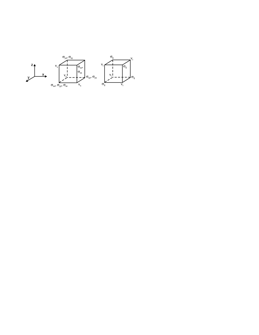
FIG. 1.: Unit cell of the three-dimensional staggered grid onto which the continuous velocity and stress fields of the elastodynamic equations are mapped in order to conserve the skew-symmetry. Left: grid for elastic isotropic solids. Note: the Lamé constants $\lambda$ and $\mu$ coincide with the stress field components, and the mass density is only defined on velocity field points. Right: grid for the general anisotropic case ($i,j=x,y,z$).

The explicit form of $H$ is derived in the appendix, in the case of a two-dimensional isotropic elastic solid. Accordingly, the discrete analogue of $\psi(t)$ is given by vector $\Psi(t)$.

The continuous problem, defined by ${\mathcal{H}}$, is now translated to a lattice problem defined by $H$:

$$\Psi(t)=\exp(tH)\Psi(0)\equiv U(t)\Psi(0).$$ (14)

or, in the time-stepping approach, we have for a small timestep $\tau$

$$\Psi(t+\tau)=\exp(\tau H)\Psi(t)=U(\tau)\Psi(t).$$ (15)

At this point, we invoke three different strategies to perform the time integration, i.e. to approximate the matrix exponential $\exp(tH)$. Here, we closely follow the derivation of algorithms to solve the time-dependent Maxwell equations [18, 19, 20, 21, 22, 23], where the problem to be solved is stated in a very similar form, although the underlying physics is different. The first algorithm is based on conserving the existing symmetries during the discretization of time, and is unconditionally stable. Here, the time integration is carried out by a time-stepping procedure. The second algorithm is based on approximating the solution itself for a particular time instance, by means of a Chebyshev expansion, and constitutes therefore a “one-step” algorithm. The last algorithm is based on recasting the original velocity-stress finite-difference algorithm into matrix exponential form. This allows to remove the staggered-in-time nature, and offers an elegant way to derive higher-order in time algorithms. The construction of the algorithms is briefly repeated in the next section.

III The matrix exponential approach

A Unconditionally stable algorithms

A sufficient condition for an algorithm to be unconditionally stable is that [25]

$$\|U(\tau)\Psi(t)\|\leq\|\Psi(t)\|.$$ (16)

Since $U(\tau)$ is an orthogonal transformation (see previous section), we have $\|U(\tau)\Psi(t)\|=\|\Psi(t)\|$, and it is sufficient to conserve the orthogonality of $U(t)$ for an approximation $\tilde{U}(t)$ to $U(t)$, in order to construct an unconditionally stable algorithm. One way to accomplish this is to make use of the Lie-Trotter-Suzuki formula [26, 27] and generalizations thereof [28, 29]. If the matrix $H$ is decomposed, so that ${H}=\sum_{i=1}^{p}{H}_{i}$, then

$$U_{1}(\tau)=e^{\tau{H}_{1}}\ldots e^{\tau{H}_{p}},$$ (17)

is a first order approximation to $U(\tau)$. More importantly, if each matrix $H_{i}$ is skew-symmetric, then $U_{1}(\tau)$ is orthogonal by construction, and hence, algorithms based on $U_{1}(\tau)$, are unconditionally stable. Using the fact that both $U(\tau)$ and $U_{1}(\tau)$ are orthogonal matrices, the error on $U_{1}(\tau)$ is subject to the upper bound [30]

$$\|U(\tau)-U_{1}(\tau)\|\leq\frac{\tau^{2}}{2}\sum_{i<j}^{p}\|[{H}_{i},{H}_{j}]\|\,,$$ (18)

where $[{H}_{i},{H}_{j}]=H_{i}H_{j}-H_{j}H_{i}$.

In the appendix, the decomposition of $H$ is carried out for two-dimensional isotropic elastic solids, for which $p=12$, and it is shown that each matrix $H_{i}$ is block diagonal. The computation of the matrix exponential of a block diagonal matrix $H_{i}$ can be performed efficiently, as it is equal to the block-diagonal matrix of the matrix exponentials of the individual blocks. Therefore, the numerical calculation of $e^{\tau H_{i}}$ reduces to the calculation of matrix exponentials of $2\times 2$ matrices, which are rotations.

In practice, implementation of the first order algorithm is all that is required to construct higher order algorithms. This is due to the fact that in the product-formula approach, the accuracy of an approximation can be improved in a systematic way by reusing lower order approximations, without changing the fundamental symmetries. For example, the orthogonal matrix

$$U_{2}(\tau)={U_{1}(-\tau/2)}^{T}U_{1}(\tau/2)=e^{\tau{H}_{p}/2}\ldots e^{\tau{H}_{1}/2}e^{\tau{H}_{1}/2}\ldots e^{\tau{H}_{p}/2},$$ (19)

is a second-order approximation to $U(\tau)$ [28, 29]. A particularly useful fourth-order approximation (applied in for example  [18, 19, 27, 28, 29, 30, 31, 32, 33, 34, 35, 36, 37, 38, 39]) is given by [28]

$$U_{4}(\tau)=U_{2}(a\tau)U_{2}(a\tau)U_{2}((1-4a)\tau)U_{2}(a\tau)U_{2}(a\tau),$$ (20)

where $a=1/(4-4^{1/3})$.

B One-step algorithm

A well-known alternative for timestepping is to use Chebyshev polynomials to construct approximations to time-evolution operators [40, 41, 42, 43, 44]. This approach has also been successfully applied to the problem of seismic wave propagation [14, 16]. However, the main differences between these implementations and the algorithm explained below, besides the spatial discretization (which is based here on a central difference approximation, instead of a spectral method), is that in the present case, matrix $H$ is explicitly anti-symmetrized, which gives rise to purely imaginary eigenvalues [45]. This is an important property to justify the validity of the expansion. In the derivation of the current algorithm, we follow [20, 21, 22], a recent implementation of the Chebyshev algorithm to solve electromagnetic wave propagation.

The basic idea is to expand the time evolution matrix $U(t)=\exp(tH)$ for a specific time instance $t$ in matrix valued Chebyshev polynomials on the domain of eigenvalues of $H$, which lies entirely on the imaginary axis since $H$ is skew-symmetric. For proper application of the expansion, the domain of eigenvalues is rescaled to $[-1,1]$, by considering the matrix $B=-iH/\|H\|_{1}$, where $\|H\|_{1}$ denotes the 1-norm of the matrix. It is given by $\|H\|_{1}\equiv\max_{j}\sum_{i}|H_{ij}|$, see [45], and is easy to compute since the matrix $H$ is sparse. Operating on state $\Psi(0)$, the expansion becomes

$$\Psi(t)=\exp(tH)\Psi(0)=\exp(izB)\Psi(0)=\left[J_{0}(z)I+2\sum_{n=1}^{\infty}J_{n}(z)\widetilde{T}_{n}(B)\right]\Psi(0),$$ (21)

where $I$ is the identity matrix, $z=t\|H\|$, $J_{n}$ are $n$th order Bessel functions and $\widetilde{T}_{n}(B)=i^{n}T_{n}(B)$ are the modified Chebyshev polynomials, defined by the recursion relation

$$\widetilde{T}_{0}(B)\Psi(0) =\Psi(0),$$ (22a)

$$\widetilde{T}_{1}(B)\Psi(0) =iB\Psi(0),$$ (22b)

$$\widetilde{T}_{n+1}(B)\Psi(0) =2iB\widetilde{T}_{n}(B)\Psi(0)+\widetilde{T}_{n-1}(B)\Psi(0)\quad\text{for $n\geq 1$}.$$ (22c)

Due to the fact that the matrix $B$ is purely imaginary, it follows from the above recursion relation (22) that $\widetilde{T}_{n}(B)\Psi(0)$ and thus $\Psi(t)$ will be real valued and no complex arithmetic is involved, as should be the case.

In practice, the summation in Eq. (21) will be truncated at some expansion index $m$. This number depends on the value of $z$, since the amplitude of the coefficients $J_{n}(z)$ decrease exponentially for $n>z$; this is explained in more detail in Refs. [20, 21, 22]. Consequently, the computation of one timestep amounts to carrying out $m$ repetitions of recursion relation Eq. (22) to obtain the final state. This is a simple procedure: only the multiplication of a vector with a sparse matrix and the summation of vectors are involved.

C A modified VS-FDTD algorithm

In section III A, it was shown that in the product formula formalism, higher-order in time algorithms can be constructed by reusing the lower order algorithms. This elegant technique to increase the accuracy of time integration can also be applied to FDTD algorithms (in case of the Maxwell Equations, see [23]), and hence the conventional VS-FDTD algorithm, if it is recast into an exponent operator form.

The update equations of the VS-FDTD [7, 8] algorithm can be written as

$$\left(\begin{array}[]{c}{\mathbf{\sigma}}(t+\tau)\\ {\mathbf{v}}(t+\tau/2)\end{array}\right)=(I+\tau A)(I+\tau B)\left(\begin{array}[]{c}{\mathbf{\sigma}}(t)\\ {\mathbf{v}}(t-\tau/2)\end{array}\right)\equiv U_{1}(\tau)\left(\begin{array}[]{c}{\mathbf{\sigma}}(t)\\ {\mathbf{v}}(t-\tau/2)\end{array}\right),$$ (23)

where

$$A=\left(\begin{array}[]{cc}0&-CD^{T}\\ 0&0\end{array}\right),$$ (24)

and

$$B=\left(\begin{array}[]{cc}0&0\\ \frac{1}{\rho}D&0\end{array}\right).$$ (25)

Since $A^{2}=B^{2}=0$, the time evolution operator $U_{1}(\tau)$ is equal to

$$U_{1}(\tau)=\exp(\tau A)\exp(\tau B),$$ (26)

and second-order accurate in time operating on fields that are defined staggered-in-time. However, if $U_{1}(\tau)$ is interpreted as an approximation to the operator $\exp(\tau A+\tau B)$, working on fields non staggered-in-time, it is a first-order approximation. Furthermore, since the time evolution operator is now expressed in matrix exponential form, the accuracy can be increased by the same procedure as was used for the unconditionally stable algorithms (cf. eqs. (19) and (20)). Therefore, the operator

$$U_{2}(\tau)=\exp(\tau A/2)\exp(\tau B)\exp(\tau A/2),$$ (27)

constitutes a second-order approximation to the exact time evolution operator. And similarly, a fourth order algorithm can be derived, see Eq. (20).

So, by introducing a small modification to the original VS-FDTD algorithm, that would require a minimal change in existing numerical codes, the staggered-in-time nature is removed, and higher-order in time algorithms are derived.

IV Sources

In the presence of an explosive initial condition, or other time-dependent body force, the equation of motion reads

$$\frac{\partial}{\partial t}\psi(t)={\mathcal{H}}\psi(t)+\phi(t),$$ (28)

where the time-dependent source is denoted by the term $\phi(t)$. The formal solution is given by

$$\psi(t)=\exp(t{\mathcal{H}})\psi(0)+\int_{0}^{t}\exp((t-u){\mathcal{H}})\phi(u)du.$$ (29)

In the time-stepping approach (e.g. the unconditionally stable algorithms), the source term –if its time dependence is known explicitly– can be integrated for each timestep. For example, a standard quadrature formula can be employed to compute the integral over $u$, like the fourth-order accurate Simpson rule [47]

$$\int_{t}^{t+\tau}e^{(t+\tau-u){\mathcal{H}}}\phi(u)\,du\approx\frac{\tau}{6}\left(e^{\tau H}\phi(t)+4e^{\tau H/2}\phi(t+\tau/2)+\phi(t+\tau)\right).$$ (30)

In case of the one-step algorithm, this approach of incorporating the source term is not efficient, as for each value of $t-u$ the recursion (22) would have to be performed, and a different route is taken. Instead, each of the two terms on the right hand side of equation (29) is expanded in modified Chebyshev polynomials separately. The expansion of the first term is discussed in section III B. For the second term, the source-term integral, the procedure is carried out here for a source with Gaussian time dependence,

$$\phi(t)=f(t)S({\mathbf{r}})=\exp(-\alpha(t-t_{0})^{2})S({\mathbf{r}}),$$ (31)

where $S({\mathbf{r}})$ denotes the spatial dependence of the source.

The source term

$$h(t,t_{0},\alpha,H)=\int_{0}^{t}due^{(t-u)H}f(u),$$ (32)

is expanded in modified Chebyshev polynomials,

$$h(t,t_{0},\alpha,H)S({\mathbf{r}})=\left(\frac{1}{2}b_{0}I+\sum_{k=0}^{K}b_{k}\widetilde{T}_{k}\right)S({\mathbf{r}}),$$ (33)

where the expansion coefficients are given by

$$b_{k}=i^{-k}\frac{2}{\pi}\int_{0}^{\pi}h(t,t_{0},\alpha,\cos\theta)\cos k\theta d\theta.$$ (34)

The replacement of $H$ by $\cos\theta$ emphasizes that $H$ should be normalized such that all eigenvalues lie in the range $[-1,1]$. We proceed by evaluating $h(t,t_{0},\alpha,H)$. After substitution of $z=\|H\|_{1}$, $z_{0}=t_{0}\|H\|_{1}$, $\beta=\alpha/\|H\|_{1}^{2}$ and $x=-iH/\|H\|_{1}$ normalize the matrix $H$, we obtain

$$h(z,z_{0},\beta,x)=\frac{1}{2}\sqrt{\frac{\pi}{\alpha}}\exp\left((z-z_{0})ix-x^{2}/4\beta\right)\left[{\operatorname{erf}}\left(z_{0}\sqrt{\beta}-\frac{ix}{2\sqrt{\beta}}\right)+{\operatorname{erf}}\left((z-z_{0})\sqrt{\beta}+\frac{ix}{2\sqrt{\beta}}\right)\right].$$ (35)

Now we put $x=\cos\theta$ and the remaining integral over $\theta$ in equation (34) is computed by a Fast Fourier transformation:

$$b_{k}=2i^{-k}\sum_{n=0}^{N-1}e^{2\pi ink/N}h(z,z_{0},\beta,\cos\frac{2\pi n}{N}).$$ (36)

The derivation of the Chebyshev expansion coefficients for a source defined by equation

$$g(t)=\frac{\partial}{\partial t}f(t)=-2\alpha(t-t_{0})\exp(-\alpha(t-t_{0})^{2}).$$ (37)

is very similar, and will not be treated explicitly here.

V Results

The performance and accuracy of the algorithms introduced in the previous sections is studied by comparing the results with a reference solution generated by the one-step algorithm, denoted by $\hat{\Psi}(t)$. This choice is motivated by the fact that the latter, considering the time integration, produces numerically exact results [14, 16, 41]. Furthermore, there are rigorous bounds on the error of the unconditionally stable algorithm (cf. Eq. (18)): in the presence of a source $\phi(t)$, the difference between the exact solution $\Psi(t)$ and the approximate solution $\tilde{\Psi}(t)$, obtained by using the 4th order unconditionally stable algorithm, is bounded by [23]

$$\|\Psi(t)-\tilde{\Psi}(t)\|\leq c_{4}t\tau^{4}\left(\|\Psi(0)\|+\int_{0}^{t}du\|\phi(u)\|\right),$$ (38)

where $c_{4}$ is a constant. For the difference between the exact solution and the solution obtained by using the one-step algorithm, we can write using the triangle inequality

$$\|\Psi(t)-\hat{\Psi}(t)\|\leq\|\Psi(t)-\tilde{\Psi}(t)\|+\|\tilde{\Psi}(t)-\hat{\Psi}(t)\|.$$ (39)

Using equations (38) and (39) and the fact that the difference $\|\tilde{\Psi}(t)-\hat{\Psi}(t)\|$ vanishes with $\tau^{4}$, as we will show below, we can be confident that the one-step algorithm indeed produces numerically exact results. This justifies to define the error as $\|\tilde{\Psi}(t)-\hat{\Psi}(t)\|/\|\hat{\Psi}(t)\|)$.

The performance of the following algorithms is considered: the original VS-FDTD algorithm, denoted by Vir; the unconditionally stable algorithms, denoted by LTS-2 and LTS-4, for resp. second and fourth order accuracy in time; the non staggered-in-time, modified VS-FDTD algorithm, denoted by VNS-2 and VNS-4, depending on the accuracy in time.

Consider a rectangular system consisting of two different materials, displayed in figure 2.

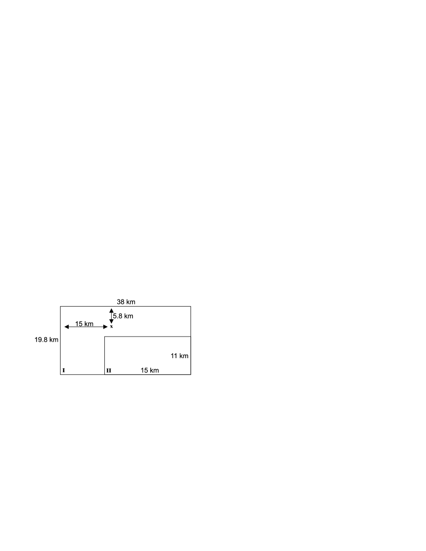
FIG. 2.: The corner-edge system, consisting of two different materials. The system size and location of the source (x) are indicated in the picture. At the top, a free-surface boundary condition is imposed, the other boundaries are rigid. The overall density is $\rho=2500$ kgm^-3, and the mesh size is $\delta=100$ m. In the bulk material (I), the wave velocities are $v_{p}=6$ kms^-1 and $v_{s}=2$ kms^-1, whereas in the inner material (II), they are $v_{p}=9$ kms^-1 and $v_{s}=3$ kms^-1. The source excites the $s_{xx}$ and $s_{yy}$ stress fields with time dependence $g(t)$ from equation (37) and parameters $\alpha=40$ and $t_{0}=1.5$ s.

This system is also studied in references [8, 10], and proved to be a good testing situation for the performance of an algorithm solving the elastodynamic equations. The time evolution of the velocity and stress fields is computed using an explosion as initial condition, modeled by equation (37), up to $t=6$ s, with the six different algorithms. In figure 3, the kinetic-energy density distribution is shown for two different time instances.

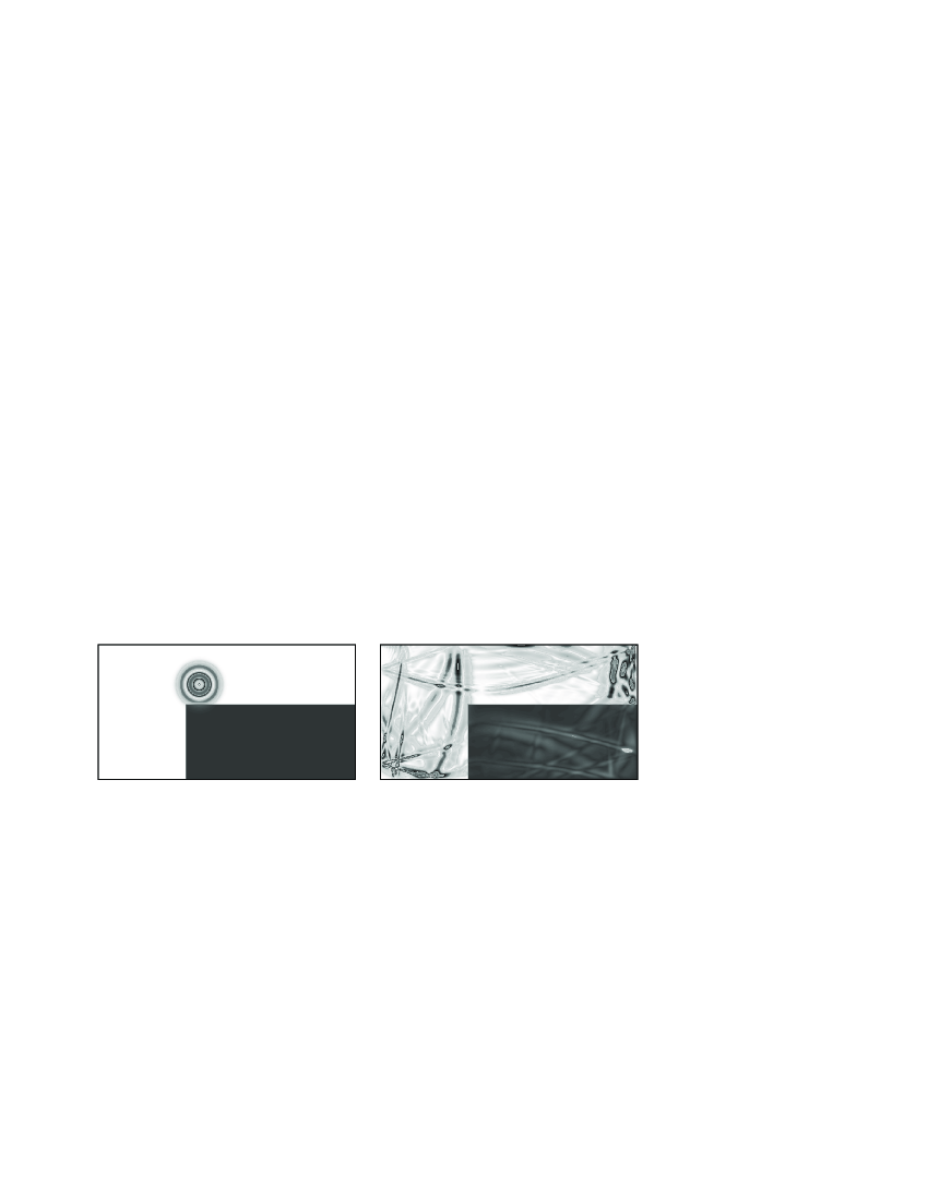
FIG. 3.: Two snapshots of the kinetic-energy density distribution of the corner-edge system of figure 2. Left: state at $t=1.8$ s, right: state at $t=6.0$ s.

For the corner-edge system, the errors are listed in table I, and are shown in figure 4.

Time-step (s)	Vir	VNS-2	VNS-4	LTS-2	LTS-4
$5\cdot 10^{-2}$	$\infty$	$\infty$	$\infty$	$3.0\cdot 10^{0}$	$3.1\cdot 10^{0}$
$5\cdot 10^{-3}$	$1.7\cdot 10^{-2}$	$1.7\cdot 10^{-2}$	$4.1\cdot 10^{-6}$	$5.9\cdot 10^{-1}$	$1.6\cdot 10^{-4}$
$5\cdot 10^{-4}$	$1.7\cdot 10^{-4}$	$1.7\cdot 10^{-4}$	$4.1\cdot 10^{-10}$	$6.1\cdot 10^{-3}$	$1.6\cdot 10^{-8}$
$5\cdot 10^{-5}$	$1.7\cdot 10^{-6}$	$1.7\cdot 10^{-6}$	$2.0\cdot 10^{-13}$	$6.1\cdot 10^{-5}$	$2.0\cdot 10^{-10}$
$5\cdot 10^{-6}$	$1.7\cdot 10^{-8}$	$1.7\cdot 10^{-8}$	$2.8\cdot 10^{-13}$	$6.1\cdot 10^{-7}$	-

TABLE I.: Error as function of timestep for all timestepping algorithms, for the system defined in figure 2. An infinite symbol ($\infty$) denotes that the algorithm was not stable, whereas in one case (-) the computation was not performed. The error in the staggered-in-time Vir algorithm is determined by averaging the error in the kinetic and potential energy density at respectively the final time instance and the final time instance shifted by half a timestep. The time shifting procedure is carried out by the Chebyshev algorithm and also applied to prepare the initial condition.

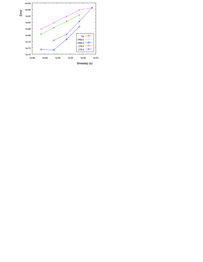
FIG. 4.: Error as function of timestep for all timestepping algorithms, for the system defined in figure 2, using the data from table I.

For the largest timestep, the VS-FDTD algorithms (Vir,VNS-2,VNS-4) are unstable. This can be expected, since the maximum timestep is limited by the largest velocity, the $v_{p}$ velocity, and the mesh-size, through the Courant limit [8]

$$\tau<\frac{\delta}{v_{p}\sqrt{2}}.$$ (40)

Furthermore, from table I it is clear that for all algorithms the error scales according to the order of accuracy in time. We also see that for the corner-edge system, the VS-FDTD algorithms perform much better than the energy-conserving LTS algorithms, as long as the timestep is smaller than the Courant limit. For timesteps larger than the Courant limit, the LTS algorithms (LTS-2 and LTS-4) are stable, although the error does not (yet) scale according to the order of accuracy in time [48]. For very accurate results (errors below $10^{-10}$), the number of operations the achieve this accuracy becomes so large that the error does not scale systematic anymore.

With respect to the efficiency of the algorithms, we note that the number of matrix-vector operations $W$, necessary to perform one timestep, is 1 for the Vir algorithm, 1.5 for the second-order VNS-2 and LTS-2 algorithms, and 10 for the fourth-order VNS-4 and LTS-4 algorithms. For the specific example here, the corner-edge system, the one-step algorithm employs $m=1514$ expansion terms. At $t=6$ and $\tau=0.005$, the VNS-2 algorithm already uses more (namely 1800) matrix-vector operations. Therefore, we draw the conclusion that one-step algorithm should be preferred to be used to solve the time evolution for this problem. Note that in general, the choice of which algorithm to use depends heavily on which degree of error is acceptable. In this specific case, there are values for $\tau$ for which the VNS-2 algorithm uses less matrix-vector operations than the one-step algorithm, but then the error will be larger than the error for $\tau=0.005$, and maybe unacceptably high. On the other hand, one VNS-2 or LTS-2 matrix-vector operation is carried out (in practice) faster than one Chebyshev recursion iteration, although this depends on the actual implementation.

It is important to note that the initial condition plays an important role in the error of the solution produced by a specific algorithm. From the results of the corner-edge system, one might draw the conclusion that the VS-FDTD algorithms achieve better results than the LTS algorithms for all systems. This is not true. In table II, the error is listed as function of timestep for all algorithms, as compared with the one-step algorithm, for a system consisting of a random medium (also studied in for example [49]) and starting from a random initial condition. The results are also shown in figure 5. From the table and the figure, it is clear that in this case, the LTS family of algorithms perform better than the VS-FDTD algorithms. Again we see that the error scales according to the order of accuracy in time, except for very small errors (below $10^{-10}$). Especially for the LTS-4 algorithm, we see that accumulation of rounding errors, due to large number of operations, increases the error.

Time-step (s)	Vir	VNS-2	VNS-4	LTS-2	LTS-4
$5\cdot 10^{-2}$	$\infty$	$\infty$	$\infty$	$1.2\cdot 10^{0}$	$5.8\cdot 10^{-2}$
$5\cdot 10^{-3}$	$1.3\cdot 10^{-1}$	$1.3\cdot 10^{-1}$	$1.6\cdot 10^{-5}$	$5.4\cdot 10^{-2}$	$1.3\cdot 10^{-5}$
$5\cdot 10^{-4}$	$1.3\cdot 10^{-3}$	$1.3\cdot 10^{-3}$	$1.6\cdot 10^{-9}$	$5.4\cdot 10^{-4}$	$1.4\cdot 10^{-9}$
$5\cdot 10^{-5}$	$1.3\cdot 10^{-5}$	$1.3\cdot 10^{-5}$	$1.6\cdot 10^{-13}$	$5.4\cdot 10^{-6}$	$1.7\cdot 10^{-11}$
$5\cdot 10^{-6}$	$1.3\cdot 10^{-7}$	$1.3\cdot 10^{-7}$	$1.1\cdot 10^{-13}$	$5.4\cdot 10^{-8}$	$1.7\cdot 10^{-10}$

TABLE II.: Error as function of timestep for all timestepping algorithms. In this case, the one-step algorithm employs $m=321$ expansion terms. The system measures $L_{x}=L_{y}=10$, with a mesh of $\delta=0.1$, and the material parameters $\rho,\lambda,\mu$ vary randomly in space with values distributed randomly in the interval $[1,3]$. The error is determined at $t=3$. (all quantities are expressed here in dimensionless units).

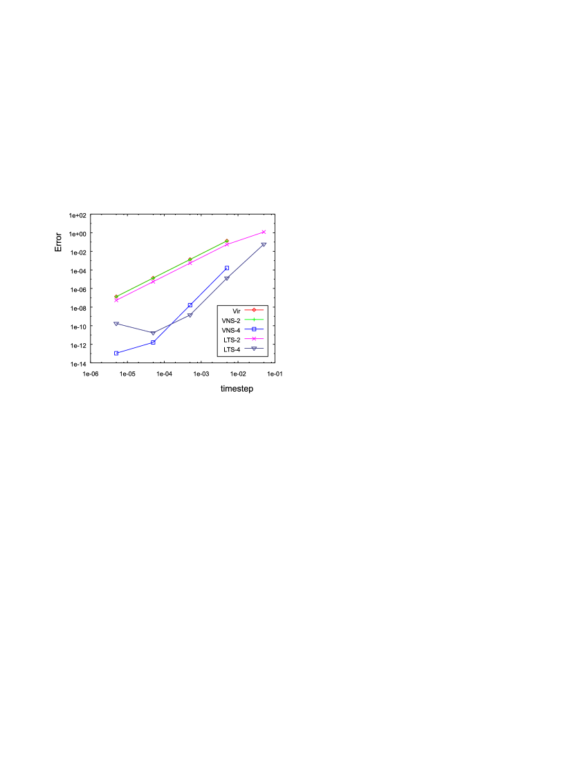
FIG. 5.: Error as function of timestep for all timestepping algorithms, for a random medium and random initial conditions, using the data from table II.

VI Conclusions

In this paper, we have introduced algorithms to solve the time-dependent elastodynamic equations, based on a matrix exponential approach. The conservation of the underlying skew-symmetry of the first-order partial differential equations while discretizing the spatial operators and fields, offers a sound starting point to expand the time evolution operator in Chebyshev polynomials. The resulting one-step algorithm is accurate up to machine precision, and this statement is justified by rigorous bounds on the error of the unconditionally stable algorithms. The latter class of algorithms proved particularly useful if the total energy should be conserved or if a random initial condition is used.

Finally, the original VS-FDTD algorithm is modified by recasting it into an exponent operator form. In this new formulation, the staggered-in-time nature is removed and higher-order in time algorithms are derived, based on the lower-order algorithms. Existing VS-FDTD codes can be modified with minor effort to benefit from these advantages.

In this paper, only free and rigid boundary conditions are considered. Future research is aimed at incorporating absorbing boundary conditions, and the presence of visco-elastic materials. More sophisticated discretization schemes, conserving the skew-symmetry, can be easily incorporated [19], and do not require conceptual changes.

Appendix: discretization and decomposition of ${\mathcal{H}}$ for two-dimensional isotropic elastic solids

In this appendix, it is shown how the matrix

$${\mathcal{H}}=\left(\begin{array}[]{cc}0&-\sqrt{C}D^{T}\frac{1}{\sqrt{\rho}}\\ \frac{1}{\sqrt{\rho}}D\sqrt{C}&0\end{array}\right),$$ (41)

is discretrized conserving its skew-symmetric properties, for two dimensional isotropic elastic solids. In two dimensional P-SV wave propagation, no dependency upon $y$ is assumed. For isotropic elastic solids, the stiffness matrix is given in terms of the Lamé coefficients $\lambda$ and $\mu$ by [24]

$$C=\left(\begin{array}[]{ccc}\lambda+2\mu&\lambda&0\\ \lambda&\lambda+2\mu&0\\ 0&0&\mu\end{array}\right),$$ (42)

in the basis ${\mathbf{\sigma}}=(\sigma_{xx},\sigma_{zz},\sigma_{xz})^{T}$. In the skew-symmetric basis, using the variables ${\mathbf{w}}=\sqrt{\rho}\,{\mathbf{v}}$ and ${\mathbf{s}}=C^{-1/2}{\mathbf{\sigma}}$, one needs $\sqrt{C}$, which reads

$$\sqrt{C}=\left(\begin{array}[]{ccc}\alpha&\beta&0\\ \beta&\alpha&0\\ 0&0&\sqrt{\mu}\end{array}\right),$$ (43)

where

$$\alpha =\frac{1}{\sqrt{2}}\left(\sqrt{\lambda+\mu}+\sqrt{\mu}\right),$$ (44)

$$\beta =\frac{1}{\sqrt{2}}\left(\sqrt{\lambda+\mu}-\sqrt{\mu}\right).$$ (45)

This gives for the explicit form of the matrix ${\mathcal{H}}$

$${\mathcal{H}}=\left(\begin{array}[]{ccc|cc}0&0&0&\alpha\frac{\partial}{\partial x}\frac{1}{\sqrt{\rho}}&\beta\frac{\partial}{\partial z}\frac{1}{\sqrt{\rho}}\\ 0&0&0&\beta\frac{\partial}{\partial x}\frac{1}{\sqrt{\rho}}&\alpha\frac{\partial}{\partial z}\frac{1}{\sqrt{\rho}}\\ 0&0&0&\sqrt{\mu}\frac{\partial}{\partial z}\frac{1}{\sqrt{\rho}}&\sqrt{\mu}\frac{\partial}{\partial x}\frac{1}{\sqrt{\rho}}\\ \hline\cr\frac{1}{\sqrt{\rho}}\frac{\partial}{\partial x}\alpha&\frac{1}{\sqrt{\rho}}\frac{\partial}{\partial x}\beta&\frac{1}{\sqrt{\rho}}\frac{\partial}{\partial z}\sqrt{\mu}&0&0\\ \frac{1}{\sqrt{\rho}}\frac{\partial}{\partial z}\beta&\frac{1}{\sqrt{\rho}}\frac{\partial}{\partial z}\alpha&\frac{1}{\sqrt{\rho}}\frac{\partial}{\partial x}\sqrt{\mu}&0&0\\ \end{array}\right),$$ (46)

in the basis $\psi=(s_{xx},s_{zz},s_{xz},w_{x},w_{z})^{T}$. The discrete analogue of $\psi$, the vector $\Psi$, is obtained by mapping the fields onto the two-dimensional staggered grid [8] that is shown in figure 6.

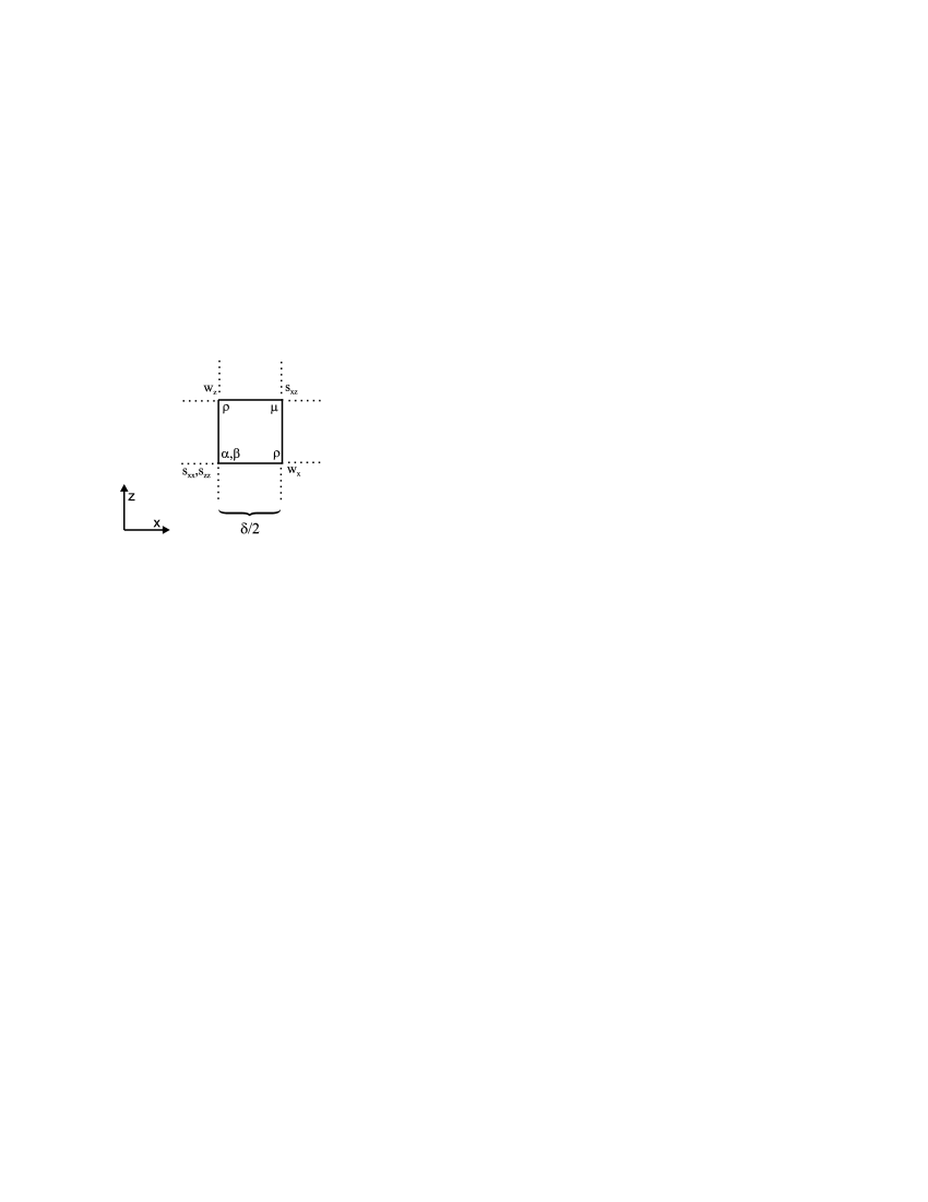
FIG. 6.: Unit cell of the two dimensional staggered grid onto which the continuous velocity and stress fields of the elastodynamic equations are mapped in order to conserve the skew-symmetry.

We adopt the convention that the $s_{xx}$ and $s_{zz}$ stress fields are located in the $(1,1)$ corner of the grid. The values of the discretized fields $f$ are related to their continuous counterparts $g$ by

$$f(i,j,t)=g(i\delta/2,j\delta/2,t).$$ (47)

Therefore, using the unit vector ${\mathbf{e}}(i,j,k)$, fields within the vector $\Psi$ can be indexed on the grid by

$$\Psi(i,j,s_{xx},t)\equiv{\mathbf{e}}^{T}_{i,j,s_{xx}}\Psi(t)\equiv s_{xx}(i,j,t),$$ (48)

and analogous equations apply for indexing the other stress and velocity fields within $\Psi$.

Due to the staggered nature of the grid and the choice of the origin, the $s_{xx}$ and $s_{zz}$ stress fields are only defined on the $x=$odd and $z=$odd lattice points. Similarly, the $w_{x}$ and $w_{z}$ velocity fields are defined at respectively the $x=$even/$z=$odd and $x=$odd/$z=$even lattice points, and the $s_{xz}$ stress field is given at the $x=$even and $z=$even grid entries. Note that all for simplicity of notation the fields are indexed on the full grid, despite the fact that they are not defined on each point.

It is assumed that the total number of lattice points in each direction is odd, and also that the boundary is located at the first and last rows/columns of the grid. The free or rigid boundary conditions themselves are implemented by excluding the field points that are located at the boundary and should remain zero during the time integration.

Using this grid and the central-difference approximation to the spatial derivative, we obtain the spatially discretized analogue of equation (46), for example

$$\frac{\partial}{\partial t}s_{xx}(i,j,t)=\alpha(i,j)\frac{1}{\delta}\left[\frac{w_{x}(i+1,j,t)}{\sqrt{\rho(i+1,j)}}-\frac{w_{x}(i-1,j,t)}{\sqrt{\rho(i-1,j)}}\right]+\beta(i,j)\frac{1}{\delta}\left[\frac{w_{z}(i,j+1,t)}{\sqrt{\rho(i,j+1)}}-\frac{w_{z}(i,j-1,t)}{\sqrt{\rho(i,j-1)}}\right],$$ (49)

and

$$\frac{\partial}{\partial t}w_{x}(i,j,t) =\frac{\alpha(i+1,j)s_{xx}(i+1,j,t)-\alpha(i-1,j)s_{xx}(i-1,j,t)}{\delta\sqrt{\rho(i,j)}}$$ (50)

$$+\frac{\beta(i+1,j)s_{zz}(i+1,j,t)-\beta(i-1,j)s_{zz}(i-1,j,t)}{\delta\sqrt{\rho(i,j)}}$$ (51)

$$+\frac{\sqrt{\mu(i,j+1)}s_{xz}(i,j+1,t)-\sqrt{\mu(i,j-1)}(s_{xz}(i,j-1,t)}{\delta\sqrt{\rho(i,j)}}.$$ (52)

Similar equations hold for $s_{zz},s_{xz}$ and $w_{z}$. Using this notation, the matrix $H$ can be decomposed into

$$H=H^{(x,s_{xx},w_{x})}+H^{(x,s_{zz},w_{x})}+H^{(x,s_{xz},w_{z})}+H^{(z,s_{xx},w_{z})}+H^{(z,s_{zz},w_{z})}+H^{(z,s_{xz},w_{x})},$$ (53)

where, for instance, the explicit form of $H^{(x,s_{xx},w_{x})}$ is given by

$$H^{(x,s_{xx},w_{x})} =\mathop{{\sum}^{\prime}}_{j=1}^{n_{y}}\mathop{{\sum}^{\prime}}_{i=1}^{n_{x}-2}\frac{\alpha(i+1,j)}{\delta\sqrt{\rho(i,j)}}\left[{\mathbf{e}}^{\phantom{T}}_{i,j,s_{xx}}{\mathbf{e}}^{T}_{i+1,j,w_{x}}-{\mathbf{e}}^{\phantom{T}}_{i+1,j,w_{x}}{\mathbf{e}}^{T}_{i,j,s_{xx}}\right]$$ (54)

$$+\mathop{{\sum}^{\prime}}_{j=1}^{n_{y}}\mathop{{\sum}^{\prime}}_{i=2}^{n_{x}-1}\frac{\alpha(i,j)}{\delta\sqrt{\rho(i+1,j)}}\left[{\mathbf{e}}^{\phantom{T}}_{i,j,s_{xx}}{\mathbf{e}}^{T}_{i+1,j,w_{x}}-{\mathbf{e}}^{\phantom{T}}_{i+1,j,w_{x}}{\mathbf{e}}^{T}_{i,j,s_{xx}}\right]$$ (55)

$$=H_{1}^{(x,s_{xx},w_{x})}+H_{2}^{(x,s_{xx},w_{x})}.$$ (56)

Here, the prime in the summation indicates that the summation index is increased with strides of two. It is easy to convince oneself that the matrices $H_{1}^{(x,s_{xx},w_{x})}$ and $H_{2}^{(x,s_{xx},w_{x})}$ are block diagonal and skew-symmetric. The other matrices in equation (53) have similar explicit forms and can also be decomposed into block diagonal parts. Therefore, a first-order approximation to the matrix exponent, as given by equation (17), reads

$$\exp(\tau H)=$$ (57)

$$\quad\quad\phantom{\cdot}\exp\left(\tau H_{1}^{(x,s_{xx},w_{x})}\right)\exp\left(\tau H_{2}^{(x,s_{xx},w_{x})}\right)\exp\left(\tau H_{1}^{(x,s_{zz},w_{x})}\right)\exp\left(\tau H_{2}^{(x,s_{zz},w_{x})}\right)$$ (58)

$$\quad\quad\cdot\exp\left(\tau H_{1}^{(x,s_{xz},w_{z})}\right)\exp\left(\tau H_{2}^{(x,s_{xz},w_{z})}\right)\exp\left(\tau H_{1}^{(z,s_{xx},w_{z})}\right)\exp\left(\tau H_{2}^{(z,s_{xx},w_{z})}\right)$$ (59)

$$\quad\quad\cdot\exp\left(\tau H_{1}^{(z,s_{zz},w_{z})}\right)\exp\left(\tau H_{2}^{(z,s_{zz},w_{z})}\right)\exp\left(\tau H_{1}^{(z,s_{xz},w_{x})}\right)\exp\left(\tau H_{2}^{(z,s_{xz},w_{x})}\right)$$ (60)

$$\quad\quad+{\mathcal{O}}(\tau^{2}).$$ (61)

REFERENCES

- [1] J. Lysmer and L. Drake, “A finite element method for seismology”, in Methods in Computational Physics 11 (Academic Press, New York, 1972).
- [2] H. Boa et al, “Large-scale simulation of elastic wave propagation in heterogenous media on parallel computers”, Comp. Meth. appl. Mech. Eng. 152, 85–102, (1998).
- [3] A.T. Patera, “A spectral method for fluid dynamics: laminar flow in a channel expansion”, J. Comput. Phys. 54, 468–488, (1984).
- [4] D. Komatitsch, “Méthodes spectrales et éléments spectraux pour l’équation de l’élastodynamique 2D et 3D en milieu hétérogène”, PhD thesis, Institute de Physique du Globe de Paris, Paris (1997).
- [5] P. Fellinger et al, “Numerical modeling of elastic wave propagation and scattering with EFIT - elastodynamic finite integration technique”, Wave Motion 21, 47–66, (1995).
- [6] G.V. Konyukh, Y.V. Kritsov and B.G. Mikhailenko, “Numerical-analytical algorithm of seismic wave propagation in inhomogeneous media”, Appl. Math. Lett. 11, 99–104, (1998).
- [7] J. Virieux, “SH-wave propagation in heterogeneous media: velocity-stress finite difference method”, Geophysics 49, 1933–1957, (1984).
- [8] J. Virieux, “P-SV wave propagation in heterogeneous media: velocity-stress finite difference method”, Geophysics 51, 889–901, (1986).
- [9] A.R. Levander, “Fourth-order finite-difference P-SV seismograms”, Geophysics 53, 1425–1436 (1988).
- [10] K.R. Kelly et al, “Synthetic seismograms: a finite difference approach”, Geophysics 41, 2–27, (1976).
- [11] M.A. Dablain, “The application of high-order differencing to the scalar wave equation”, Geophysics 51, 54–66, (1987).
- [12] H. Igel, P. Mora and B. Riollet, “Anisotropic wave propagation through finite-difference grids”, Geophysics 60, 1203–1216 (1995).
- [13] D. Kosloff and E. Baysal, “Forward modeling by a Fourier method”, Geophysics 47, 1402–1412, (1982).
- [14] H. Tal-Ezer, D. Kosloff and Z. Koren, “An accurate scheme for seismic forward modelling”, Geophys. Prosp. 35, 479–490, (1987).
- [15] E.H. Saenger, N. Gold and S.A. Shapiro, “Modeling the propagation of elastic waves using a modified finite-difference grid”, Wave Motion 31, 77–92, (2000).
- [16] H. Tal-Ezer, J.M. Carcione and D. Kosloff, “An accurate and efficient scheme for wave propagation in linear viscoelastic media”, Geophysics 55, 1366–1379, (1990).
- [17] I. Oprs̆al and J. Zahradník, “From unstable to stable seismic modeling by finite-difference method”, Phys. Chem. Earth (A) 24, 247–252, (1999).
- [18] J.S. Kole, M.T. Figge and H. De Raedt, “Unconditionally stable methods to solve the time-dependent Maxwell Equations”, Phys. Rev. E 64, 066705-1–066705-14, (2001).
- [19] J.S. Kole, M.T. Figge and H. De Raedt, “Higher-order nconditionally stable methods to solve the time-dependent Maxwell Equations”, Phys. Rev. E 65, 066705-1–066705-12, (2002).
- [20] H. De Raedt, K. Michielsen, J.S. Kole, and M.T. Figge, “Chebyshev Method to solve the Time-Dependent Maxwell Equations”, to appear in Computer Simulation Studies in Condensed-Matter Physics XV, D.P. Landau et al. (Eds.), Springer Proceedings in Physics, (Springer, Berlin, 2002).
- [21] H. De Raedt, J.S. Kole, K. Michielsen and M.T. Figge, “Solving the Maxwell Equations by the Chebyshev method: A one-step finite-difference time-domain algorithm”, preprint available at http://arxiv.org/abs/physics/0208060.
- [22] H. De Raedt, J.S. Kole, K. Michielsen and M.T. Figge, “One-step finite-difference time-domain algorithm to solve the Maxwell Equations”, submitted to Phys. Rev. E.
- [23] H. De Raedt, J.S. Kole, K. Michielsen and M.T. Figge, “Numerical methods for solving the time-dependent Maxwell Equations”, preprint available at http://arxiv.org/abs/physics/02010035.
- [24] L.D. Landau and E.M. Lifshitz, Theory of Elasticity, (Pergamon Press, Oxford, 1986).
- [25] G.D. Smith, Numerical solution of partial differential equations, (Clarendon, Oxford, 1985).
- [26] H.F. Trotter, “On the product of semi-groups of operators”, Proc. Am. Math. Soc. 10, 545–551, (1959).
- [27] M. Suzuki, S. Miyashita, and A. Kuroda, “New method of Monte Carlo simulations and phenomenological theory”, Prog. Theor. Phys. 58, 1377–1387, (1977).
- [28] M. Suzuki, “Decomposition formulas of exponential operators and Lie exponentials with some applications to quantum physics”, J. Math. Phys. 26, 601–612, (1985); ibid, “General theory of fractal path integrals with applications to many-body theories and statistical physics”, J. Math. Phys. 32, 400–407, (1991).
- [29] H. De Raedt and B. De Raedt, “Applications of the generalized Trotter formula”, Phys. Rev. A 28, 3575–3580, (1983).
- [30] H. De Raedt, “Product formula algorithms for solving the time dependent Schrödinger equation”, Comp. Phys. Rep. 7, 1–72, (1987).
- [31] A.J. Chorin, T.J.R. Hughes, M.F. McCracken, and J.E. Marsden, “Product formulas and numerical algorithms”, Comm. Pure Appl. Math. 31, 205–256, (1978).
- [32] H. Kobayashi, N. Hatano, and M. Suzuki, “Study of correction terms for higher-order decompositions of exponential operators”, Physica A 211, 234–254, (1994).
- [33] H. De Raedt, K. Michielsen, “Algorithm to solve the time-dependent Schrödinger equation for a charged particle in an inhomogeneous magnetic field: Application to the Aharonov-Bohn effect”,Comp. in Phys. 8, 600–607, (1994).
- [34] A. Rouhi, J. Wright, “Spectral implementation of a new operator splitting method for solving partial differential equations”, Comp. in Phys. 9, 554–563, (1995).
- [35] B.A. Shadwick and W.F. Buell, “Unitary integration: a numerical technique preserving the structure of the quantum Liouville equation”, Phys. Rev. Lett. 79, 5189–5193, (1997).
- [36] M. Krech, A. Bunker, and D.P. Landau, “Fast spin dynamics algorithms for classical spin systems”, Comp. Phys. Comm. 111, 1–13, (1998).
- [37] P. Tran, “Solving the time-dependent Schrödinger equation: suppression of reflection from the grid boundary with a filtered split-operator approach”, Phys. Rev. E 58, 8049–8051, (1998).
- [38] K. Michielsen, H. De Raedt, J. Przeslawski, and N. Garcia, “Computer simulation of time-resolved optical imaging of objects hidden in turbid media”, Phys. Rep. 304, 89–144, (1998).
- [39] H. De Raedt, A.H. Hams, K. Michielsen, and K. De Raedt, “Quantum computer emulator”, Comp. Phys. Comm. 132, 1–20, (2000).
- [40] C. Leforestier, R.H. Bisseling et al, “A comparison of different propagation schemes for the time-dependent Schrödinger equation”, J. of Comp. Physics 94, 59–80, (1991).
- [41] H. Tal-Ezer, “Spectral methods in time for hyperbolic equations”, SIAM. J. Numer. Anal. 23, 11–26, (1986).
- [42] Y.L. Loh, S.N. Taraskin and S.R. Elliot, “Fast time-evolution method for dynamical systems”, Phys. Rev. Lett. 84, 2290–2293, (2000).
- [43] T. Itaka et. al., “Calculating the linear response functions of noninteracting electrons with a time-dependent Schrödinger equation”, Phys. Rev. E 56, 1222–1229, (1997).
- [44] R.N. Silver and H. Röder, “Calculation of densities of states and spectral functions by Chebyshev recursion and maximum entropy”, Phys. Rev. E 56, 4822–4829, (1997).
- [45] J.H. Wilkinson, The Algebraic Eigenvalue Problem, (Clarendon Press, Oxford, 1965).
- [46] M. Abramowitz and I. Stegun, Handbook of mathematical functions, (Dover, New York, 1964).
- [47] K.E. Atkinson, An introduction to numerical analysis, (Wiley, New York, 1989).
- [48] This behavior is also noticed when unconditionally stable algorithms are used to solve the time-dependent Maxwell Equations, see [19].
- [49] G. Kneip and C. Kerner, “Accurate and efficient seismic modeling in random media”, Geophysics 58, 576–588, (1993).