Theory of dark resonances for alkali vapors in a buffer-gas cell

Abstract

We develop an analytical theory of dark resonances that accounts for the full atomic-level structure, as well as all field-induced effects such as coherence preparation, optical pumping, ac Stark shifts, and power broadening. The analysis uses a model based on relaxation constants that assumes the total collisional depolarization of the excited state. A good qualitative agreement with experiments for Cs in Ne is obtained.

I Introduction

Nonlinear interference effects connected with the atomic ground state coherence are now well known and widely used Arimondo (1996a). One of the most promising classes of these effects, especially for precise measurements, is that of super-narrow dark resonances Wynands and Nagel (1999); Kitching et al. (2000); Stähler et al. (2001) that appear in the medium’s response to bichromatic laser excitation, when the laser frequency difference is close to the atomic ground-state splitting. The use of vapor cells containing a buffer gas in addition to an alkali vapor has allowed the measurement of resonance linewidths less than 50 Hz Brandt et al. (1997); Erhard and Helm (2001). While such resonances have been extensively investigated experimentally (especially in the case of Cs) Wynands and Nagel (1999), a detailed theoretical understanding is not yet well developed for realistic multilevel systems, motivating the present work. Our theory was developed in close connection with ongoing efforts to construct compact atomic clocks Kitching et al. (2000); Knappe et al. (2001); Kitching et al. (2001, 2002) and magnetometers Wynands and Nagel (1999); Stähler et al. (2001). For any practical application of dark resonances, the stability and accuracy are optimized with respect to parameters such as the output signal amplitude, width, and shift. In the problem considered here, many parameters, such as laser detunings, field component polarizations and amplitudes, and buffer gas pressure, affect the dark resonance itself. In addition, various excitation schemes (for example, $D_{2}$ versus $D_{1}$ line excitation Stähler et al. (2002)) and different atomic isotopes can be used. A natural question arises: what design will optimize the performance of the clock (or magnetometer)? Previous theories did not completely answer this question. One main obstacle was connected with the complicated energy-level structure of the real atomic systems used in experiments.

Generally speaking, there are several types of problems in the theoretical description of dark resonances. One problem relates to a proper treatment of the relaxation processes in the system, including velocity-changing collisions Arimondo (1996b) and the spatial diffusion of coherently prepared atoms Vanier and Audoin (1989); Zibrov and Matsko (2001). Light propagation through coherently prepared nonlinear media, especially through optically thick media Lukin et al. (1997), can be thought of as another type of difficulty. This paper addresses another important problem: that of field-induced processes in multilevel systems such as coherence preparation, optical pumping, ac Stark shifts, and power broadening. All existing theories can be classified into three kinds: few-state models (basically, three-state lambda systems) Ling et al. (1996); Grishanin et al. (1998); Erhard and Helm (2001), perturbation theories Wynands et al. (1998), and numerical simulations Ling et al. (1996); Erhard and Helm (2001). All three classes of theories have disadvantages. The first theory neglects many details of the actual configuration of atomic levels. Perturbation theory neglects some effects induced by the presence of the optical field (namely, optical pumping, ac Stark shifts, and power broadening). Numerical simulation theories demonstrate a lack of genuine understanding and predictive power.

This paper presents a new analytical theory, that accounts for the level structure (both Zeeman and hyperfine) of a real atom, as well as all field-induced effects. The relaxation processes are treated in the simplest way: by neglecting velocity-changing collisions and all effects connected with the spatial inhomogeneity, we reduce the model to one described simply by relaxation constants. The crucial assumption is total collisional depolarization of the excited state. In addition, we add the (optional) approximations of homogeneous broadening and low saturation. With these approximations, a general analytical result is obtained for the atomic response, which result is valid for arbitrary excitation schemes ($D_{2}$ as well as $D_{1}$ lines), light field polarizations, and magnetic fields. In the specific case of circularly polarized light in the presence of a magnetic field, where only two states participate in the coherence preparation, analytical lineshapes (generalized Lorentzian) coincide exactly with the phenomenological model heuristically introduced previously to fit experimental data Knappe et al. . In the case of zero magnetic field, and when contributions of different Zeeman sub-states are well overlapped, the resonance lineshape is also approximately described by the generalized Lorentzian. A comparison of analytically calculated coefficients of the Lorentz-Lorenz model (with no free parameters) with coefficients extracted from experimental data demonstrates a good qualitative agreement.

II Statement of the problem

In this section, the general framework of the problem is described, the basic assumptions we make are stated and the specific procedure for calculating the quantities of interest is outlined. We consider the resonant interaction of alkali atoms in the $S_{1/2}$ ground state with a two-frequency laser field

$${\bf E}(z,t)={\bf E}_{1}\exp[-i(\omega_{1}t-k_{1}z)]+{\bf E}_{2}\exp[-i(\omega_{2}t-k_{2}z)]+c.c.\;,$$ (1)

where both components propagate in the positive direction ($k_{1,2}>0$). The field can excite atoms either to the $P_{1/2}$ state ($D_{1}$ line) or to the $P_{3/2}$ state ($D_{2}$ line). Two hyperfine (HF) components are present in the ground state with the total angular momenta $F_{1}=I+1/2$ and $F_{2}=I-1/2$ (where $I$ is the nuclear spin). The HF splitting in the ground state $\Delta=({\cal E}_{1}-{\cal E}_{2})/\hbar$ is in the range $1$ to $10\,$GHz. The excited state has two ($D_{1}$ line) or four ($D_{2}$ line) HF levels with the angular momenta $F_{e}=I-J_{e},\ldots,I+J_{e}$ and the energies ${\cal E}_{e}=\hbar\omega_{e}$. The HF splitting of the excited state is typically one order of magnitude smaller than $\Delta$. To be more specific, we assume that the frequency $\omega_{1}$ is close to resonance with the $F_{1}\to F_{e}$ transitions, while the other frequency $\omega_{2}$ is close to the frequencies of the $F_{2}\to F_{e}$ transitions. Thus, we have a $\Lambda$-type excitation scheme (Fig. 1). In the absence of an external B-field, the HF levels are degenerate with respect to the total angular momentum projections. For the Zeeman sub-states the following shorthand notations will be used: $|e\rangle=|F_{e},\,m_{e}\rangle$ with $m_{e}=-F_{e},\ldots,F_{e}$, and $|i,m\rangle=|F_{i},\,m\rangle$ with $m=-F_{i},\ldots,F_{i}$ ($i=1,2$).

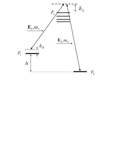
Figure 1: Excitation scheme

For simplicity, we consider first an atom at rest, positioned at the origin $z=0$. Each frequency component of the field can in principal induce transitions from both ground-state HF levels. Then the interaction Hamiltonian in the dipole approximation contains contributions of two kinds:

$$\widehat{H}_{D-E}=-\sum_{e,i,m}|e\rangle\langle e|(\widehat{\bf d}\cdot{\bf E}_{i})|i,m\rangle\langle i,m|-\sum_{e,i\neq j,m}|e\rangle\langle e|(\widehat{\bf d}\cdot{\bf E}_{i})|j,m\rangle\langle j,m|e^{-i(\omega_{i}-\omega_{j})t}+h.c.\;,$$ (2)

where we use a rotating frame (the unitary transformation of the ground-state basis $|i,m\rangle\to\exp(i\omega_{i}t)|i,m\rangle$), and $\widehat{\bf d}$ is the dipole moment operator. The first term in (2) is independent of time in the rotating basis, and we refer to it as the resonant contribution. The second term, oscillating at the difference frequency, results in off-resonant contributions to the optical shifts and optical pumping rates, as well as in temporal oscillations of the atomic density matrix. The role of the off-resonant term in the case of a three-level $\Lambda$ system has been studied in great detail Grishanin et al. (1998). The amplitudes of the oscillating parts of the density matrix can be approximated as $|dE|^{2}/(\hbar\Delta)^{2}$. For the moderate field intensities considered here ($<10\,$mW/cm²) this ratio is very small, $|dE|^{2}/(\hbar\Delta)^{2}\sim 10^{-6}-10^{-8}$, and the oscillating terms can be safely neglected. However, the off-resonant contributions to the optical energy shifts and widths can be significant, especially in the case of large one-photon detunings.

The Hamiltonian for a free atom in the rotating frame can be written as

$$\widehat{H}_{0}=-\sum_{e}\hbar(\delta_{L}-\omega_{e})|e\rangle\langle e|-\hbar\frac{\delta_{R}}{2}\sum_{m}(|1,m\rangle\langle 1,m|-|2,m\rangle\langle 2,m|)\;.$$ (3)

Here $\delta_{L}=(\delta_{1}+\delta_{2})/2$ is the average one-photon detuning, $\delta_{L}$ and $\omega_{e}$ are measured from a common zero level (for example, from the HF level with maximal momentum $F_{e}=I+J_{e}$), and $\delta_{R}=\delta_{2}-\delta_{1}=\omega_{2}-\omega_{1}-\Delta$ is the Raman (two-photon) detuning.

Since this paper is concerned with the field-induced effects in multi-level atomic systems, the relaxation processes are modeled by several constants. The homogeneous broadening of the optical line, due mainly to collisions with a buffer gas, is described by the constant $\gamma$. We assume that the excited state is completely depolarized due to collisions during the radiative lifetime $\tau_{e}$, i.e., the depolarization rates $\gamma_{\kappa}$ obey the condition

$$\gamma_{\kappa}\,\tau_{e}\gg 1\;.$$ (4)

The relaxation of the ground-state density matrix to the isotropic equilibrium, both due to the diffusion through the laser beam and due to collisions, is modeled by a single constant $\Gamma$.

Under the assumption of moderate field intensities and high buffer-gas pressure, we develop the theory in the low-saturation limit:

$$\frac{|dE|^{2}}{\hbar^{2}}\ll\frac{\gamma}{\tau_{e}}\;.$$ (5)

The two-photon dark resonance appears when the Raman detuning $\delta_{R}$ is scanned around zero. The width of the dark resonance, which is related to the ground-state relaxation, is usually six orders of magnitude smaller than the optical linewidth $\gamma$. The approximation $\delta_{R}\ll\gamma$ is therefore suitable.

It should be stressed that all approximations are well justified for typical experimental conditions. For example, in the case of Cs in a background Ne atmosphere at a pressure of $p=10\,$kPa, the homogeneous broadening $\gamma\approx 2\pi\,860\,$MHz Allard and Kielkopf (1982) of the optical line exceeds the Doppler width $k\overline{v}\approx 2\pi\,300\,$MHz, so velocity-changing collisions are inconsequential. The collisional depolarization rate $\gamma_{\kappa}\approx 2\pi\,70\,$MHz Happer (1972) is large compared to the inverse radiative lifetime $1/\tau_{e}=2\pi\,5.3\,$MHz. The Rabi frequency $|dE|/\hbar\approx 1/\tau_{e}$ for the field intensity $8.8\,$mW/cm², which results in a saturation parameter $(|dE|/\hbar)^{2}\,\tau_{e}/\gamma\approx 10^{-2}$. The two-photon detuning is scanned in the range $|\delta_{R}|<2\pi\,1\,$MHz, and the ground-state relaxation rate can be estimated to be $\Gamma\approx 2\pi\,53\,$Hz Beverini et al. (1971); Vanier and Audoin (1989).

Eliminating optical coherences with these approximations (for details see the Appendix), we arrive at the following set of equations for the ground-state density submatrix ($\widehat{\sigma}_{gg}=\widehat{\Pi}_{g}\widehat{\sigma}\widehat{\Pi}_{g}$):

$$\frac{d}{dt}\widehat{\sigma}_{gg}=-i\left[\widehat{H}_{\rm eff}\widehat{\sigma}_{gg}-\widehat{\sigma}_{gg}{\widehat{H}_{\rm eff}}^{\dagger}\right]+\left(\frac{\pi_{e}}{\tau_{e}}+\Gamma\right)\,\frac{\widehat{\Pi}_{g}}{n_{g}},$$ (6)

$${\rm Tr}\{\widehat{\sigma}_{gg}\}=1\;,$$ (7)

where $\widehat{\Pi}_{g}=\sum_{m}(|1,m\rangle\langle 1,m|+|2,m\rangle\langle 2,m|)$ is the ground-state projector, $n_{g}=2(2I+1)$ is the total number of sub-states in the ground state, and $\pi_{e}$ is the total population of the excited state. The first term ($\propto\pi_{e}$) of the source in (6) corresponds to the isotropic repopulation of the ground-state sublevels due to the spontaneous decay of the excited states. The other term ($\propto\Gamma$) describes the entrance of unpolarized atoms due to diffusion and collisions. Due to the conservation of the total number of particles (7), separate dynamic equations for the excited-state density matrix elements are not needed. Both the dynamics and steady state are completely governed by the non-Hermitian ground-state Hamiltonian:

$$\widehat{H}_{\rm eff}=-\frac{\delta_{R}}{2}\sum_{m}(|1,m\rangle\langle 1,m|-|2,m\rangle\langle 2,m|)+\widehat{R}-i\frac{\Gamma}{2}\,\widehat{\Pi}_{g}\;.$$ (8)

Here the excitation matrix,

$$\widehat{R} = \sum_{i,j,e,m,m^{\prime}}|i,m\rangle\frac{\langle i,m|{(\widehat{\bf d}\cdot{\bf E}_{i})}^{\dagger}|e\rangle\langle e|(\widehat{\bf d}\cdot{\bf E}_{j})|j,m^{\prime}\rangle}{\hbar^{2}\,[(\delta_{L}-\omega_{e})+i\gamma/2]}\langle j,m^{\prime}|+$$ (9)

$$+ \sum_{i\neq j,e,m,m^{\prime}}|i,m\rangle\frac{\langle i,m|{(\widehat{\bf d}\cdot{\bf E}_{j})}^{\dagger}|e\rangle\langle e|(\widehat{\bf d}\cdot{\bf E}_{j})|i,m^{\prime}\rangle}{\hbar^{2}\,[(\delta_{L}+\omega_{j}-\omega_{i}-\omega_{e})+i\gamma/2]}\langle i,m^{\prime}|,$$

contains the resonant (first summation) as well as off-resonant (second summation) contributions to the optical shifts and optical pumping rates (Hermitian and anti-Hermitian parts, respectively). The non-diagonal ($i\neq j$) elements of the resonant term induce the Raman coherence between the HF levels of the ground state responsible for the dark resonance.

The generic matrix element in (9) is calculated from the Wigner-Eckart theorem:

$$\langle i,m_{i}|{(\widehat{\bf d}\cdot{\bf E}_{k})}^{\dagger}|e\rangle\langle e|(\widehat{\bf d}\cdot{\bf E}_{l})|j,m_{j}\rangle=|\langle J_{e}||d||J_{g}\rangle|^{2}\,r(F_{e},F_{i})\,r(F_{e},F_{j})\times$$ (14)

$$\times\,\sum_{K,\,q}(-1)^{F_{e}+F_{j}+K}\left\{\begin{array}[]{rcl}1&1&K\\ F_{i}&F_{j}&F_{e}\end{array}\right\}\sqrt{2K+1}\,(-1)^{F_{i}-m_{i}}\left(\begin{array}[]{rcl}F_{i}&K&F_{j}\\ -m_{i}&q&m_{j}\end{array}\right)\{{{\bf E}_{k}}^{*}\otimes{\bf E}_{l}\}_{K\,q}\;,$$

where $\langle J_{e}||d||J_{g}\rangle$ is the reduced matrix element of the dipole moment and

$$r(F_{e},F_{i})=\sqrt{(2J_{e}+1)(2F_{e}+1)(2F_{i}+1)}\,\left\{\begin{array}[]{rcl}J_{g}&J_{e}&1\\ F_{e}&F_{i}&I\end{array}\right\}$$

is the partial coupling amplitude of the $F_{i}\to F_{e}$ transition. In the general case we have scalar ($K=0$), vector ($K=1$) and quadrupole ($K=2$) contributions. All possible selection rules are contained in the coefficients of vector coupling, i.e., the $6j$ and $3jm$ symbols.

For an atom moving along the direction of propagation of the optical field, the field frequencies are shifted due to the Doppler effect: $\omega_{i}\to\omega_{i}-k_{i}v$. As a result, a Doppler shift of the one-photon detuning $\delta_{L}\to\delta_{L}-kv$ occurs, where $k=(k_{1}+k_{2})/2$, as does a residual Doppler shift of the Raman detuning $\delta_{R}\to\delta_{R}-(k_{2}-k_{1})v$. At high buffer-gas pressure the residual Doppler shift is suppressed due to the Lamb-Dicke effect Dicke (1953); Vanier and Audoin (1989). However, in the general case the Doppler shift of the one-photon detuning can be significant, and certain quantities must be averaged over the Maxwell velocity distribution. Nevertheless, for buffer-gas pressures typically used in experiments, the approximation of homogeneous broadening is reasonable as a first approach to the problem, because the homogeneous width $\gamma$ equals or even exceeds the Doppler width $k\overline{v}$.

Here we consider the steady-state regime, setting $(d/dt)\,\widehat{\sigma}_{gg}=0$ in (6). As a spectroscopic signal, we consider the total excited-state population $\pi_{e}$, which is proportional to the total light absorption in optically thin media or to the total fluorescence. The following procedure is used to find $\pi_{e}$. From (6), the ground-state density matrix $\widehat{\sigma}_{gg}$ is expressed in terms of $\pi_{e}$, and then $\pi_{e}$ is calculated from the normalization condition (7). The solution of this algebraic problem can be obtained in a compact analytical form in two important special cases. The first arises when both field components have the same simple (circular or linear) polarization and there is no magnetic field. Here, for a suitable choice of the quantization axis, the excitation matrix $\widehat{R}$ contains only diagonal elements with respect to the magnetic quantum number, i.e., $m=m^{\prime}$ in (9). The second case appears when a magnetic field is applied and just a few substates contribute to the Raman coherence for arbitrary light polarizations and arbitrary magnetic field directions. Both cases are considered below.

III Simple light polarization, no magnetic field

We turn now to the case of circular field polarization when the quantization axis is directed orthogonal to the polarization vector (or alternatively linear polarization when the quantization axis is aligned along the polarization vector). We evaluate the total excited-state population, $\pi_{e}$, in order to determine how the dark resonance signal (proportional to $\pi_{e}$) depends on parameters such as the optical detuning from resonance. Under these assumptions, the complete set of equations (6) can be split into independent blocks for each magnetic quantum number $m$ ($m$-blocks). These blocks for $m=\pm F_{1}$ contain only one equation for the sub-state population $\pi^{(\pm F_{1})}$. The other blocks with $m\neq\pm F_{1}$ contain four equations (two for the populations and two for the Raman coherences), corresponding to an effective two-level system with the upper $|1,m\rangle$ and lower $|2,m\rangle$ states (Fig. 2). The parameters of the two-level system are expressed in terms of matrix elements of $\widehat{R}$ as follows: the population relaxation rates $\widetilde{\Gamma}_{i}=\Gamma+R^{(m)}_{i}$ include the optical pumping rates $R^{(m)}_{i}=2\,{\rm Im}\{\langle i,m|\widehat{R}|i,m\rangle\}$; the dephasing rate is $\widetilde{\Gamma}_{12}=(\widetilde{\Gamma}_{1}+\widetilde{\Gamma}_{2})/2$; the effective detuning $\widetilde{\delta}_{R}=\delta_{R}-(S^{(m)}_{1}-S^{(m)}_{2})$ includes optical shifts $S^{(m)}_{i}={\rm Re}\{\langle i,m|\widehat{R}|i,m\rangle\}$; and the coherence between levels is excited by the complex coupling $V-iU=\langle 1,m|\widehat{R}|2,m\rangle$. Note that the phase of the matrix element $\langle 1,m|{(\widehat{\bf d}\cdot{\bf E}_{1})}^{\dagger}|e\rangle\langle e|(\widehat{\bf d}\cdot{\bf E}_{2})|2,m\rangle$ can be chosen equal to zero without loss of generality, so that $\langle 2,m|\widehat{R}|1,m\rangle=\langle 1,m|\widehat{R}|2,m\rangle$.

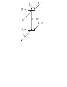
Figure 2: Effective two-level system, corresponding to one $m$-block

Both the upper and lower states are repopulated with the same rate $\beta=(\pi_{e}/\tau_{e}+\Gamma)/n_{g}$. First the total $m$-block population $\pi^{(m)}=\pi^{(m)}_{1}+\pi^{(m)}_{2}$ per unit repopulation rate is found. For the outermost blocks, $m=\pm F_{1}$, $\pi^{(\pm F_{1})}=1/(\Gamma+R^{(\pm F_{1})}_{1})$. The result for $m\neq\pm F_{1}$ is a quotient of polynomials of second order in the effective detuning,

$$\pi^{(m)}=\frac{A\,\widetilde{\delta}_{R}^{2}+B}{C\,\widetilde{\delta}_{R}^{2}+D\,\widetilde{\delta}_{R}+E}\;,$$ (15)

where

$$A = \widetilde{\Gamma}_{1}+\widetilde{\Gamma}_{2}\;;\;\;\;\;\;B=\widetilde{\Gamma}_{12}[\widetilde{\Gamma}_{12}(\widetilde{\Gamma}_{1}+\widetilde{\Gamma}_{2})+8\,V^{2}]\;;$$

$$C = \widetilde{\Gamma}_{1}\widetilde{\Gamma}_{2}\;;\;\;\;\;\;\;\;\;\;D=4\,UV(\widetilde{\Gamma}_{1}-\widetilde{\Gamma}_{2})\;;$$ (16)

$$E = \widetilde{\Gamma}_{12}^{2}\widetilde{\Gamma}_{1}\widetilde{\Gamma}_{2}+2\,\widetilde{\Gamma}_{12}(\widetilde{\Gamma}_{1}+\widetilde{\Gamma}_{2})(V^{2}-U^{2})-16\,U^{2}V^{2}\;.$$

The repopulation rate, corresponding to unit total population in all $m$-blocks is

$$\beta=\left[\sum_{m=-F_{1}}^{F_{1}}\pi^{(m)}\right]^{-1}\;,$$ (17)

and the total excited-state population is finally expressed as

$$\pi_{e}=\tau_{e}(n_{g}\,\beta-\Gamma)\;.$$ (18)

In the general case, when polarizations of the field components are different, or the same but elliptical, there is no basis where the matrices $\langle 1,m|\widehat{R}|1,m^{\prime}\rangle$, $\langle 2,m|\widehat{R}|2,m^{\prime}\rangle$, and $\langle 1,m|\widehat{R}|2,m^{\prime}\rangle$ are simultaneously diagonal. In this situation, the full equation set for the ground-state density matrix elements must be solved, including all possible Zeeman and Raman coherences. Nevertheless, one important exception should be noted. If the optical linewidth is much greater than the excited-state HF splitting $\gamma\gg(\omega_{e,\,\mathrm{max}}-\omega_{e,\,\mathrm{min}})$, the quadrupole contributions to $\widehat{R}$ are negligible Wynands et al. (1998). The vector terms are diagonal (with respect to the magnetic quantum number) in the coordinate frame with $z$ as the quantization axis, since $[{{\bf E}_{i}}^{*}\times{\bf E}_{j}]\propto{\bf e}_{z}$. Thus, we return to the case discussed above.

IV Dark resonances in a magnetic field

In a weak magnetic field, the ground-state magnetic sublevels are split due to the linear Zeeman effect, which can be described by the following additional term in the effective Hamiltonian (8):

$$\widehat{H}_{B}=\sum_{i,m}m\,\Omega_{i}\,|i,m\rangle\langle i,m|\;.$$ (19)

Here the quantization axis is directed along the magnetic field, and $\Omega_{i}=\mu_{B}g_{i}B/\hbar$ are the Zeeman splitting frequencies, with $\mu_{B}$ the Bohr magneton and $B$ the magnetic flux density. The $g$-factors of levels, $g_{i}$, are expressed through the electronic $g_{J}$ and nuclear $g_{I}$ Lande factors:

$$g_{1,2}=\pm\,\frac{g_{J}-g_{I}}{2\,I+1}+g_{I}\;.$$

The magnetic field causes a precession of atomic coherences with frequencies $m\,\Omega_{i}-m^{\prime}\,\Omega_{j}$. When the Zeeman frequencies are much larger than off-diagonal elements of the excitation matrix $\Omega_{i}\gg|\langle i,m|\widehat{R}|i,m^{\prime}\rangle|$, the light-induced Zeeman coherences within the $i$-th HF level are negligible. Thus, we again have a set of independent two-level systems, consisting of the sub-states $|1,m_{1}\rangle$ and $|2,m_{2}\rangle$ (where $|m_{1}-m_{2}|\leq 2$ due to the selection rules). The formulas (15) and (III) for the total block population are still valid for every $(m_{1},\,m_{2})$-block with the following substitutions:

$$\widetilde{\Gamma}_{i} = \Gamma+R^{(m_{i})}_{i}\;;\;\;\;\widetilde{\delta}_{R}=\delta_{R}-(S_{1}^{(m_{1})}-S_{2}^{(m_{2})})-(m_{1}\Omega_{1}-m_{2}\Omega_{2})\;;$$

$$V - iU=\langle 1,m_{1}|\widehat{R}|2,m_{2}\rangle=\langle 2,m_{2}|\widehat{R}|1,m_{1}\rangle\;.$$ (20)

If the Zeeman frequencies significantly exceed the widths $\widetilde{\Gamma}_{i}$, the Zeeman-split dark resonances are well resolved. In other words, the Raman coherence between the substates $|1,m_{1}\rangle$ and $|2,m_{2}\rangle$ is effectively induced when the precession frequency is approximately equal to the Raman detuning: $\delta_{R}\approx m_{1}\,\Omega_{1}-m_{2}\,\Omega_{2}$. This condition can be simultaneously satisfied for only a few $(m_{1},\,m_{2})$-blocks. More precisely, the nuclear Lande factor is typically three orders of magnitude smaller than the electronic Lande factor (for cesium $g_{J}/g_{I}\approx 2500$); then, with good accuracy, $\Omega_{1}=-\Omega_{2}=\Omega$ and the Zeeman shift of the dark resonance position is proportional to the sum of magnetic quantum numbers $n\Omega=(m_{1}\,+m_{2})\,\Omega$. It can be seen that, in the general case, three blocks $(m,\,m)$, $(m-1,\,m+1)$, and $(m+1,\,m-1)$ contribute to the coherence preparation for the resonances with even shifts $2\,m\,\Omega$, and two other blocks $(m-1,\,m)$ and $(m,\,m-1)$ contribute for the resonances with odd shifts $(2\,m-1)\,\Omega$. When $\delta_{R}$ is tuned around the resonance with given shift $n\,\Omega$, the repopulation rate $\beta$ can be written as

$$\beta=\left[Z+\sum_{m_{1}+m_{2}=n}\pi^{(m_{1},m_{2})}(\widetilde{\delta}_{R})\right]^{-1}\;,$$

where the first summand $Z$ does not depend on the Raman detuning:

$$Z=\sum_{m_{1}+m_{2}\neq n}\left(\frac{1}{\Gamma+R^{(m_{1})}_{1}}+\frac{1}{\Gamma+R^{(m_{2})}_{2}}\right)\;,$$

and $\pi^{(m_{1},m_{2})}$ is the total population of the $(m_{1},\,m_{2})$ block. Owing to the nuclear contribution, a further increase of the magnetic field causes the dark resonances to be eventually split into individual peaks, corresponding to each $(m_{1},\,m_{2})$-block Knappe et al. (2000).

V The resonance lineshape

We now consider the dark resonance lineshape in more detail. First, we analyze the particular case in which just two sub-states $|1,\,0\rangle$ and $|2,\,0\rangle$ participate in the Raman coherence, i.e., we consider the magnetically insensitive resonance ($m=0$) in a magnetic field. This $(0,\,0)$ resonance is of primary interest for possible clock applications Wynands and Nagel (1999); Kitching et al. (2000); Knappe et al. (2001), because it is only sensitive to a magnetic field in second order. Here the absorption signal, $n^{\prime\prime}_{DR}$, has the form:

$$n^{\prime\prime}_{DR}=\frac{\pi_{e}}{\tau_{e}\,n_{g}}=\frac{1}{Z+\pi^{(0)}(\widetilde{\delta}_{R})}-\frac{\Gamma}{n_{g}}\;;\;\;\;\;Z=\sum_{m\neq 0}\left(\frac{1}{\Gamma+R^{(m)}_{1}}+\frac{1}{\Gamma+R^{(m)}_{2}}\right)\;,$$ (21)

where $\pi^{(0)}$ is the total population of the $(m=0)$-block per unit repopulation rate (see (15) and (III)). Since $\pi^{(0)}$ is a quotient of polynomials of second order in $\delta_{R}$, the absorption can be written as the sum of an absorptive and a dispersive Lorentzian, and a constant background:

$$n^{\prime\prime}_{DR}=-C_{1}\,\frac{(\widetilde{\gamma}/2)^{2}}{(\widetilde{\gamma}/2)^{2}+(\delta_{R}-\delta_{0})^{2}}+C_{2}\,\frac{(\delta_{R}-\delta_{0})\,\widetilde{\gamma}/2}{(\widetilde{\gamma}/2)^{2}+(\delta_{R}-\delta_{0})^{2}}+\mathrm{const}\;.$$ (22)

The parameters in (22) are expressed in terms of the coefficients introduced by (III) in the following way. The dark resonance position is governed by the optical shifts and an additional term caused by the two-photon coupling between levels:

$$\delta_{0}=(S_{1}^{(0)}-S_{2}^{(0)})+x\;;\;\;\;\;x=-\frac{DZ}{2\,(A+CZ)}\;.$$ (23)

The width of dark resonance reads

$$(\widetilde{\gamma}/2)^{2}=\frac{B+EZ}{A+CZ}-x^{2}\;.$$ (24)

The amplitudes of the symmetrical and antisymmetrical Lorentzians are found from the relations

$$C_{1}(\widetilde{\gamma}/2)^{2} = \frac{BC-AE-xAD}{(A+CZ)^{2}}\;;$$ (25)

$$C_{2}\,\widetilde{\gamma}/2 = \frac{AD}{(A+CZ)^{2}}\;.$$ (26)

The background constant, $C/(CZ+A)-\Gamma/n_{g}$, corresponds to the absorption far off the two-photon resonance.

The result (22) for the resonance lineshape is quite general. In fact, it does not depend on our simplified assumptions on the relaxation processes but is valid also in the low-saturation limit for arbitrary relaxation matrix, whenever only two states participate in the coherence preparation and $\delta_{R}\ll\gamma$.

Turning to the case of zero magnetic field and simple field polarization, we proceed with the goal of determining the resonance position, width and amplitudes of the symmetrical and asymmetrical components as above. Since all Zeeman levels within a given hyperfine level are now degenerate, we rewrite the repopulation rate $\beta$ (17) as:

$$\beta=\left[Z+(2F_{2}+1)\langle\widetilde{\pi}^{(m)}(\delta_{R})\rangle_{m}\right]^{-1}\;,$$ (27)

where

$$Z=\sum_{m=-F_{1}}^{m=F_{1}}\left(\frac{1}{\Gamma+R^{(m)}_{1}}+\frac{1}{\Gamma+R^{(m)}_{2}}\right)$$

does not depend on $\delta_{R}$ and corresponds to the absorption far off the two-photon resonance; the sum of the variable parts of the $m$-block populations $\widetilde{\pi}^{(m)}(\delta_{R})$ is expressed through the average over $m$-blocks, where the average of a variable $X$ is defined as:

$$\langle X^{(m)}\rangle_{m}=\frac{1}{2F_{2}+1}\sum_{m=-F_{2}}^{m=F_{2}}X^{(m)}\;.$$

Since $\widetilde{\pi}^{(m)}(\delta_{R})$ is a quotient of polynomials of second order:

$$\widetilde{\pi}^{(m)}(\delta_{R})=\frac{a_{2}^{(m)}\delta_{R}+b_{2}^{(m)}}{\delta_{R}^{2}+a_{1}^{(m)}\delta_{R}+b_{1}^{(m)}}\;;$$

$$a_{1}^{(m)}=\frac{D}{C}-(S_{1}^{(m)}-S_{2}^{(m)})\;;\;\;\;b_{1}^{(m)}=\frac{E}{C}-(S_{1}^{(m)}-S_{2}^{(m)})\frac{D}{C}+(S_{1}^{(m)}-S_{2}^{(m)})^{2}\;;$$

$$a_{2}^{(m)}=\frac{A\,D}{C^{2}}\;;\;\;\;b_{2}^{(m)}=\frac{B\,C-A\,E+A\,D\,(S_{1}^{(m)}-S_{2}^{(m)})}{C^{2}}\;,$$ (28)

the average $\langle\widetilde{\pi}^{(m)}(\delta_{R})\rangle_{m}$ is a quotient of polynomials of order $2\,(2F_{2}+1)$. Generally this average describes a superposition of resonances with different widths and positions due to the $m$-dependent power broadening and ac Stark shifts, but if the laser detuning is not too large, $|\delta_{L}|\leq\Delta$, all resonances are well overlapped, and the average $\langle\,\widetilde{\pi}^{(m)}(\delta_{R})\rangle_{m}$ can be approximated by a quotient of polynomials of second order. Here we use the following simple procedure, where the average of a quotient is substituted by a quotient of the averages:

$$\langle\widetilde{\pi}^{(m)}(\delta_{R})\rangle_{m}\approx\alpha\frac{\langle a_{2}^{(m)}\rangle_{m}\delta_{R}+\langle b_{2}^{(m)}\rangle_{m}}{\delta_{R}^{2}+\langle a_{1}^{(m)}\rangle_{m}\delta_{R}+\langle b_{1}^{(m)}\rangle_{m}}\;,$$ (29)

and where the correction factor $\alpha$ is chosen such that the exact and approximate expressions coincide at $\delta_{R}=0$, i.e.,

$$\alpha=\frac{\langle b_{1}^{(m)}\rangle_{m}}{\langle b_{2}^{(m)}\rangle_{m}}\,\left\langle\frac{b_{2}^{(m)}}{b_{1}^{(m)}}\right\rangle_{m}\;.$$

Our approximation for $\beta$ yields an error less than a few percent across a wide range of parameters. With this approximation, we return to the resonance lineshape (22), where the parameters are expressed in terms of the averages over $m$:

$$\delta_{0} = -\frac{\langle a_{1}^{(m)}\rangle_{m}}{2}-\frac{(2F_{2}+1)\,\alpha}{Z}\,\frac{\langle a_{2}^{(m)}\rangle_{m}}{2}$$

$$(\widetilde{\gamma}/2)^{2} = \langle b_{1}^{(m)}\rangle_{m}+\frac{(2F_{2}+1)\,\alpha}{Z}\,\langle b_{2}^{(m)}\rangle_{m}-\delta_{0}^{2}$$

$$C_{1}\,(\widetilde{\gamma}/2)^{2} = (2F_{2}+1)\,\alpha\,\frac{\langle b_{2}^{(m)}\rangle_{m}+\langle a_{2}^{(m)}\rangle_{m}\delta_{0}}{Z^{2}}$$

$$C_{2}\,(\widetilde{\gamma}/2) = (2F_{2}+1)\,\alpha\,\frac{\langle a_{2}^{(m)}\rangle_{m}}{Z^{2}}$$

$$\mathrm{const} = \frac{1}{Z}-\frac{\Gamma}{n_{g}}\;.$$ (30)

VI Comparison with experiment

The analytical lineshape (22) coincides exactly with the phenomenological model heuristically introduced previously to fit experimental data Knappe et al. . In those experiments a vertical-cavity surface-emitting laser (VCSEL) was modulated at the 9.2-GHz hyperfine splitting frequency of the cesium atom, so that the laser output spectrum contained modulation sidebands at this frequency. Using the carrier and one of the sidebands the dark resonance could be prepared and spectroscopically observed, as a function of the detuning $\delta_{L}$ of the laser frequency from optical resonance. Data was taken for three different power ratios of carrier and sideband, with the cesium atoms contained in a cell with 8.7 kPa of neon as a buffer gas. Detection used a modulation technique that allowed to extract simultaneously the absorption and the dispersion line shape Wynands and Nagel (1999). For each detuning $\delta_{L}$, both line shapes were simultaneously fitted by the model function (22), with $C_{1}$, $C_{2}$, $\widetilde{\gamma}$, and $\delta_{0}$ as free parameters. Actually, as far as the line shapes themselves are concerned, this is a two-parameter fit: $C_{2}/C_{1}$ and $\widetilde{\gamma}$ describe the shape, and the rest the overall amplitude and position of the dark line.

Since these experimental data for Cs in Ne are fitted by (22) quite well, we can compare analytically calculated coefficients of the generalized Lorentzian to those extracted from experimental data. The dependence of the coefficients on the total light intensity ${\cal I}\propto|E_{1}|^{2}+|E_{2}|^{2}$ is almost trivial, at least when the power broadening $(R_{1}^{(m)}+R_{2}^{(m)})/2$ exceeds the dephasing rate $\Gamma$ in zero field: all the parameters $C_{1}$, $C_{2}$, $\delta_{0}$, and $\widetilde{\gamma}$ scale as ${\cal I}$. Thus, the most representative test is provided by the dependence of the coefficients on the one-photon detuning $\delta_{L}$, and on the intensity ratio ${\cal R}=|E_{1}|^{2}/|E_{2}|^{2}$ between the two field components. Such comparisons with experimental fit parameters from Knappe et al. are presented in Figs. 3 to 6, where $C_{1}$, $C_{2}$, $\delta_{0}$, and $\widetilde{\gamma}$ are plotted as functions of $\delta_{L}$ for three different relative intensities, ${\cal R}$. The other parameters used in the calculations correspond to the experimental conditions: excitation by $\sigma^{+}$ polarized radiation, total intensity ${\cal I}=0.4\,$mW/cm², optical linewidth $\gamma=2\pi\,750\,$MHz, and ground-state relaxation rate $\Gamma=2\pi\,150\,$Hz. We use no free parameters, just a single trivial scaling factor for $C_{1}$ and $C_{2}$, and a constant offset for $\delta_{0}$ that accounts for the collisional shift of the dark resonance position.

Figure 3: Absorptive coefficient, $C_{1}$, versus optical detuning, $\delta_{L}$. Plots a), b) and c) are for ${\cal R}=2.4,\,7.2,\,22$, respectively. The solid lines indicate the theoretical predictions while the points indicate the experimental data taken from Knappe et al. .

Figure 4: Dispersive coefficient, $C_{2}$, versus optical detuning, $\delta_{L}$. Plots a), b) and c) are for ${\cal R}=2.4,\,7.2,\,22$, respectively. The solid lines indicate the theoretical predictions while the points indicate the experimental data.

Figure 5: Frequency shift, $\delta_{0}$, versus optical detuning, $\delta_{L}$. Plots a), b) and c) are for ${\cal R}=2.4,\,7.2,\,22$, respectively. The solid lines indicate the theoretical predictions while the points indicate the experimental data.

Figure 6: Dark resonance width, $\widetilde{\gamma}$, versus optical detuning, $\delta_{L}$. Plots a), b) and c) are for ${\cal R}=2.4,\,7.2,\,22$, respectively. The solid lines indicate the theoretical predictions while the points indicate the experimental data.

We see a good qualitative agreement, especially for the resonance position $\delta_{0}$ and for the width $\widetilde{\gamma}$. There are some noticeable discrepancies for the amplitudes $C_{1}$ and $C_{2}$. In particular, we can see that the theoretical curve for $C_{1}$ can cross the zero level at large $\delta_{L}$, which can be attributed to the well-known Raman absorption, but which is not observed in the experimental data.

VII $D_{2}$ line excitation and connection to previously existing theories

In the specific case of the $D_{2}$ line of Cs at high buffer-gas pressure, the two-photon amplitudes $U$ and $V$ are much smaller than the optical pumping rates $R^{(0)}_{i}$ and the optical shifts $S^{(0)}_{i}$, respectively, because the most probable optical transitions $F_{1}\to F_{e}=I+J_{e}$ and $F_{2}\to F_{e}=I-J_{e}$ contribute to the one-photon transitions but not to the two-photon Raman coupling. Note that the ratio between $V$ and $R^{(0)}_{i}$ can be arbitrary, depending on the one-photon detuning $\delta_{L}$. As a result, the part of the absorption signal that varies with $\delta_{R}$ is small compared to the constant one, and we arrive, to lowest orders, at the following approximate expressions. The parameter

$$x\approx-\frac{D}{2\,C}=\frac{2\,(\widetilde{\Gamma}_{1}-\widetilde{\Gamma}_{2})\,U\,V}{\widetilde{\Gamma}_{1}\widetilde{\Gamma}_{2}}$$

is negligible with respect to the other contributions in $\delta_{0}$, $\widetilde{\gamma}$ and $C_{1}$. The resonance position offset and the width are approximated as

$$\delta_{0} \approx S^{(0)}_{1}-S^{(0)}_{2}$$

$$(\widetilde{\gamma}/2)^{2} \approx \frac{E}{C}\approx\widetilde{\Gamma}_{12}^{2}+\frac{(\widetilde{\Gamma}_{1}+\widetilde{\Gamma}_{2})^{2}}{\widetilde{\Gamma}_{1}\widetilde{\Gamma}_{2}}\,V^{2}\;.$$ (31)

The amplitudes $C_{1}$ and $C_{2}$ are given by (25) and (26) with $x=0$ and $\widetilde{\gamma}$ from (VII).

These results can be compared with those for a three-level $\Lambda$ system in the low-saturation limit. Our formulas (22)-(26) will describe this last case, as well, if we set $Z=0$, i.e.,

$$\delta_{0}=S^{(0)}_{1}-S^{(0)}_{2}\;;\;\;\;(\widetilde{\gamma}/2)^{2}=\frac{B}{A}=\widetilde{\Gamma}_{12}^{2}+4\,V^{2}$$

$$C_{1}(\widetilde{\gamma}/2)^{2}=\frac{BC-AE}{A^{2}}\;;\;\;\;C_{2}\,\widetilde{\gamma}/2=\frac{D}{A}\;.$$ (32)

Thus, the results are qualitatively similar (the main differences are the overestimated amplitudes $C_{1}$ and $C_{2}$), but now all parameters are unambiguously defined for the actual atomic structure.

When $C_{2}=0$ the lineshape is symmetrical, and occurs if $V=0$ or $\widetilde{\Gamma}_{1}=\widetilde{\Gamma}_{2}$. The first condition generalizes to $\delta_{L}=0$, and the second corresponds to the condition of equal Rabi frequencies in a simple $\Lambda$ system.

When $V=0$, the amplitude of the symmetrical signal is proportional to the square of the two-photon coupling:

$$C_{1}\approx\frac{2\,(\widetilde{\Gamma}_{1}+\widetilde{\Gamma}_{2})^{2}}{\widetilde{\Gamma}_{12}\,(\widetilde{\Gamma}_{1}+\widetilde{\Gamma}_{2}+Z\,\widetilde{\Gamma}_{1}\widetilde{\Gamma}_{2})^{2}}\,U^{2}\;,$$ (33)

which is a key point of the perturbative studies Wynands et al. (1998) but now, in addition, all effects of the optical pumping are accounted for in the prefactor in (33).

VIII Dark resonance position. Three possible definitions

The center position of the dark resonance in essence determines the output frequency of the frequency reference or the magnetic field indicated by the magnetometer. Especially for asymmetrical resonances, it is somewhat unclear exactly how that center position is defined. The quantity $\delta_{0}$ above is one possible definition of the resonance position, corresponding to the combined minimum of the absorptive part, and zero of the dispersive part, of the resonance described by (21).

Using (22)-(26), one can easily find another possible definition of the resonance center: the Raman detuning corresponding to minimum absorption.

$$\delta_{\mathrm{min}}=S_{1}^{(0)}-S_{2}^{(0)}+\frac{\widetilde{\Gamma}_{12}\,(\widetilde{\Gamma}_{2}-\widetilde{\Gamma}_{1})}{\widetilde{\Gamma}_{1}+\widetilde{\Gamma}_{2}}\,\frac{V}{U}\;.$$ (34)

A third possible definition is the point $y_{0}$, where the dispersion $n^{\prime}_{\mathrm{DR}}$ associated with the absorption (22) (by the Kramers-Kronig relations) is equal to zero. This is found to be

$$y_{0}=\delta_{0}-\frac{\widetilde{\gamma}}{2}\,\frac{C_{2}}{C_{1}}\;.$$ (35)

Each of these three quantities, $\delta_{\mathrm{min}}$, $y_{0}$ and $\delta_{0}$, could be considered the resonance center, depending on how the resonance is measured experimentally. In the general asymmetrical case, when $V\neq 0$ (non-zero effective one-photon detuning) and $\widetilde{\Gamma}_{1}\neq\widetilde{\Gamma}_{2}$ (unbalanced optical pumping rates), all three values are different. Even their behavior versus $\delta_{L}$ are qualitatively different (Fig. 7): near the one-photon resonance ($V=0$) the centroid $\delta_{0}$ of the Lorentzians has a dispersion-like shape, while $\delta_{\rm min}$ is rather of an absorptive nature, and $y_{0}$ has a more complicated shape of mixed type. In addition, $\delta_{0}$ and $\delta_{\rm min}$ are always finite, whereas $y_{0}$ goes to infinity at the zeros of $C_{1}$. These different dependences on optical detuning could, for example, alter the sensitivity of the frequency reference or magnetometer to the optical lock point. As a result, careful consideration must be given to the resonance detection method when designing frequency references or magnetometers based on dark resonances.

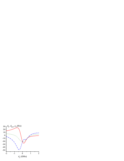
Figure 7: Three possible definitions of the dark resonance position. The centroid $\delta_{0}$ corresponds to the solid line, $\delta_{\mathrm{m}in}$ – dotted, and $y_{0}$ – dash-dotted line. All curves are calculated for the Cs $D_{2}$ line. The parameters are ${\cal I}=45\,\mu$W/cm², ${\cal R}=0.5$, and $\gamma=2\pi\,850\,$MHz.

IX Conclusion

Using very simple assumptions about the relaxation processes, analytical results can be obtained for the nonlinear absorption of bichromatic radiation near a two-photon resonance. The theory fully takes into account both the HF and the Zeeman level structures of alkali atoms as well as all light-induced effects. Our results constitute a good basis for understanding experimental works and further possible refinements of theory are possible. In particular, the case of large Doppler width $k\overline{v}>\gamma$ can be immediately studied by the substitution $\delta_{L}\to\delta_{L}-kv$ followed by averaging over the Maxwell distribution.

In addition, the theory allows for a simple parameterization of experimentally measured dark resonances in terms of absorptive and dispersive components. The theory can therefore predict, for example, the detuning for which the dispersive part of the resonance is minimized and, for a given detuning, the asymmetry in the resonance lineshape that might be expected. The analysis of the different definitions of the resonance center position is also of interest for practical applications based on dark resonances such as atomic frequency standards and magnetometers. It appears likely that the additional understanding gained by the thorough theoretical analysis presented here will lead to further refinement and development of current and future applications based on dark resonances.

Appendix A Derivation of equation (6)

In this appendix we consider in detail the derivation of the basic equation set (6). As is well-known the atomic density matrix obeys to the generalized optical Bloch equation. According to this equation, the evolution of the density matrix can be split into the two parts. The reversible one ($d/dt\,\widehat{\sigma}=-i/\hbar\,[\widehat{H},\widehat{\sigma}]$) is governed by the total Hamiltonian of an atom in a resonant external field $\widehat{H}=\widehat{H}_{0}+\widehat{H}_{D-E}$. The irreversible part originated from the interaction with environments (e.g. buffer gas or vacuum modes of electromagnetic field) are modeled by relaxation (super)operators of various kinds. The concrete form of the relaxation terms will be specified in the course of the derivation.

The first stage is the elimination of the optical coherences $\widehat{\sigma}_{eg}=\widehat{\Pi}_{e}\widehat{\sigma}\widehat{\Pi}_{g}$, where the operator $\widehat{\Pi}_{e}=\sum_{m_{e}}|F_{e},m_{e}\rangle\langle F_{e},m_{e}|$ projects on the given HF component of the excited state. In the low-saturation limit the optical coherence matrix obeys the following equation in the rotating frame:

$$\left[\frac{d}{dt}+\gamma/2-i(\delta_{L}-\omega_{e})\right]\widehat{\sigma}_{eg}=\frac{i}{\hbar}\,\left\{\sum_{i=1,2}\widehat{\Pi}_{e}(\widehat{\bf d}\cdot{\bf E}_{i})\widehat{\Pi}_{i}+\sum_{i\neq j}\widehat{\Pi}_{e}(\widehat{\bf d}\cdot{\bf E}_{i})\widehat{\Pi}_{j}e^{-i(\omega_{i}-\omega_{j})t}\right\}\widehat{\sigma}_{gg}\;.$$ (36)

On the left-hand side, the Raman detuning $\delta_{R}$ is small compared to the homogeneous width $\gamma$ ($|\delta_{R}|\ll\gamma$); $\widehat{\Pi}_{i}=\sum_{m}|F_{i},m\rangle\langle F_{i},m|$, so that $\widehat{\Pi}_{g}=\widehat{\Pi}_{1}+\widehat{\Pi}_{2}$. As is explained in the main text, the oscillations of the ground-state density submatrix $\widehat{\sigma}_{gg}$ can also be safely neglected in the rotating frame. Then, in the stationary regime ($\gamma t\gg 1$) the solution of the equation (36) is

$$\widehat{\sigma}_{eg}=\frac{i}{\hbar}\,\left\{\sum_{i=1,2}\frac{\widehat{\Pi}_{e}(\widehat{\bf d}\cdot{\bf E}_{i})\widehat{\Pi}_{i}}{\gamma/2-i(\delta_{L}-\omega_{e})}+\sum_{i\neq j}\frac{\widehat{\Pi}_{e}(\widehat{\bf d}\cdot{\bf E}_{i})\widehat{\Pi}_{j}e^{-i(\omega_{i}-\omega_{j})t}}{\gamma/2-i(\delta_{L}-\omega_{e})-i(\omega_{i}-\omega_{j})}\right\}\widehat{\sigma}_{gg}\;.$$ (37)

Under the conditions considered here, the equation for the ground-state density submatrix can be written

$$\frac{d}{dt}\widehat{\sigma}_{gg}=-\Gamma\,(\widehat{\sigma}_{gg}-\widehat{\sigma}^{(0)}_{gg})-\frac{i}{\hbar}[\widehat{H}_{0},\widehat{\sigma}_{gg}]-\frac{i}{\hbar}\left(\widehat{\Pi}_{g}\,\overline{\widehat{H}_{D-E}\,\widehat{\sigma}}\,\widehat{\Pi}_{g}-h.c.\right)+\widehat{\cal A}\{\widehat{\sigma}_{ee}\}\;,$$ (38)

where the line over operators indicates time averaging, i.e. all the oscillating terms should be removed from the product $\widehat{H}_{D-E}\,\widehat{\sigma}$. Using (37), one finds that

$$-\frac{i}{\hbar}\widehat{\Pi}_{g}\,\overline{\widehat{H}_{D-E}\,\widehat{\sigma}}\,\widehat{\Pi}_{g}=-i\,\widehat{R}\,\widehat{\sigma}_{gg}\;$$

where $\widehat{R}$ is the excitation matrix given by (9). The first term on the right-hand side of (38) describes the relaxation in the ground state (due to both diffusion and collisions) toward the equilibrium distribution outside the laser beam, $\widehat{\sigma}^{(0)}_{gg}=\widehat{\Pi}_{g}/n_{g}$. All the linear (with respect to $\widehat{\sigma}_{gg}$) terms, containing $\Gamma$, $\widehat{H}_{0}$, and $\widehat{R}$, can be combined in the effective non-Hermitian Hamiltonian (8). The last term on the right-hand side of (38) corresponds to the spontaneous radiative transfer of atoms from the excited-states, given by the density submatrix $\widehat{\sigma}_{ee}=\widehat{\cal P}_{e}\,\widehat{\sigma}\,\widehat{\cal P}_{e}$ (where $\widehat{\cal P}_{e}=\sum_{F_{e}}\widehat{\Pi}_{e}$), to the ground-state levels. Its structure will be specified below.

In the low-saturation limit, the matrix $\widehat{\sigma}_{ee}$ obeys the equation

$$\frac{d}{dt}\widehat{\sigma}_{ee}=-\frac{1}{\tau_{e}}\,\widehat{\sigma}_{ee}-\frac{i}{\hbar}[\widehat{H}_{e},\widehat{\sigma}_{ee}]-\widehat{\cal G}\{\widehat{\sigma}_{ee}\}-\frac{i}{\hbar}\left(\widehat{\cal P}_{e}\,\overline{\widehat{H}_{D-E}\,\widehat{\sigma}}\,\widehat{\cal P}_{e}-h.c.\right)\;,$$ (39)

where the first three terms on the right-hand side describe the radiative decay, the HF splitting ($\widehat{H}_{e}=\hbar\,\sum_{F_{e}}\omega_{e}\,\Pi_{e}$), and the collisional depolarization of the excited state, respectively; the last term corresponds to the excitation due to light-induced transition from the ground-state levels. This last term can be considered as a source, because it is proportional to $\widehat{\sigma}_{gg}$:

$$-\frac{i}{\hbar}\widehat{\cal P}_{e}\,\overline{\widehat{H}_{D-E}\,\widehat{\sigma}}\,\widehat{\cal P}_{e} = \frac{1}{\hbar^{2}}\sum_{F_{e},F_{e}^{\prime}}\left(\sum_{i,j}\frac{\widehat{\Pi}_{e^{\prime}}(\widehat{\bf d}\cdot{\bf E}_{i})\widehat{\Pi}_{i}\widehat{\sigma}_{gg}\widehat{\Pi}_{j}{(\widehat{\bf d}\cdot{\bf E}_{j})}^{\dagger}\widehat{\Pi}_{e}}{\gamma/2+i(\delta_{L}-\omega_{e})}+\right.$$

$$+ \left.\sum_{i\neq j}\frac{\widehat{\Pi}_{e^{\prime}}(\widehat{\bf d}\cdot{\bf E}_{i})\widehat{\Pi}_{j}\widehat{\sigma}_{gg}\widehat{\Pi}_{j}{(\widehat{\bf d}\cdot{\bf E}_{i})}^{\dagger}\widehat{\Pi}_{e}}{\gamma/2+i(\delta_{L}-\omega_{e}+\omega_{i}-\omega_{j})}\right)\;.$$

The structure of the collisional term $\widehat{\cal G}\{\widehat{\sigma}_{ee}\}$ can be found in Happer (1972). Here we simply recall that during the course of a collision only the electronic component of the atomic polarization is depolarized. The nuclear component is involved in the process of depolarization due to the HF coupling. For all alkali atoms, the excited-state HF splitting $\Delta_{e}$ is much greater than radiative decay rate $1/\tau_{e}$. In addition we assume that the collisional relaxation rates $\gamma_{\kappa}$ for the excited-state electronic multipole moments of rank $\kappa=1,\ldots,2J_{e}+1$ also obey the conditions $\gamma_{\kappa}\tau_{e}\gg 1$ (for $\kappa=0$ we assume $\gamma_{0}=0$, i.e. the collision-induced transitions between the fine structure components are not considered here). In this limit, $\Delta_{e}\tau_{e}\gg 1$ and $\gamma_{\kappa}\tau_{e}\gg 1$, the steady-state solution of (39) has particularly simple form:

$$\widehat{\sigma}_{ee}=\pi_{e}\,\frac{\widehat{\cal P}_{e}}{n_{e}}\;;\;\;\;\;\pi_{e}=\tau_{e}\left(i\,{\rm Tr}\{\widehat{R}\,\widehat{\sigma}_{gg}\}+c.c.\right)\;,$$ (40)

which corresponds to total collisional depolarization of the excited state.

Here we shall illustrate this fact in one specific case, when the excited-state HF splitting is much larger than the depolarization rates $\gamma_{\kappa}$ and when all the depolarization rates (except for $\gamma_{0}$) are the same (so-called pure electronic randomization model Happer (1972)). If $\Delta_{e}\gg\gamma_{\kappa},\,1/\tau_{e}$, one can neglect HF coherence in the excited state. For pure electronic randomization both eigenvalues and eigenvectors of the Liouvillian ${\cal G}$ are well-known Happer (1972), which allows us to write the steady-state solution of (39) for arbitrary $\gamma_{\kappa}\tau_{e}$:

$$\widehat{\sigma}_{ee} = \frac{\tau_{e}}{1+\gamma_{\kappa}\tau_{e}}\widehat{S}_{e}+\frac{\gamma_{\kappa}\tau_{e}}{1+\gamma_{\kappa}\tau_{e}}\sum_{L,M,F_{e},F_{e}^{\prime}}\frac{\tau_{e}}{1+\widetilde{\gamma}_{L}\tau_{e}}(-1)^{F_{e}-F_{e}^{\prime}}\frac{(2F_{e}+1)(2F_{e}^{\prime}+1)}{(2J_{e}+1)}\times$$ (45)

$$\times \left\{\begin{array}[]{rcl}F_{e}&F_{e}&L\\ I&I&J_{e}\end{array}\right\}\left\{\begin{array}[]{rcl}F_{e}^{\prime}&F_{e}^{\prime}&L\\ I&I&J_{e}\end{array}\right\}\widehat{T}_{LM}(F_{e}\,F_{e}){\rm Tr}\{\widehat{T}_{LM}^{\dagger}(F_{e}^{\prime}\,F_{e}^{\prime})\widehat{S}_{e}\}\;.$$

Here the source has the form

$$\widehat{S}_{e} = \frac{\gamma}{\hbar^{2}}\sum_{F_{e}}\left(\sum_{i,j}\frac{\widehat{\Pi}_{e}(\widehat{\bf d}\cdot{\bf E}_{i})\widehat{\Pi}_{i}\widehat{\sigma}_{gg}\widehat{\Pi}_{j}{(\widehat{\bf d}\cdot{\bf E}_{j})}^{\dagger}\widehat{\Pi}_{e}}{(\gamma/2)^{2}+(\delta_{L}-\omega_{e})^{2}}+\right.$$

$$+ \left.\sum_{i\neq j}\frac{\widehat{\Pi}_{e}(\widehat{\bf d}\cdot{\bf E}_{i})\widehat{\Pi}_{j}\widehat{\sigma}_{gg}\widehat{\Pi}_{j}{(\widehat{\bf d}\cdot{\bf E}_{i})}^{\dagger}\widehat{\Pi}_{e}}{(\gamma/2)^{2}+(\delta_{L}-\omega_{e}+\omega_{i}-\omega_{j})^{2}}\right)\;;$$

the relaxation rates

$$\widetilde{\gamma}_{L}=\gamma_{\kappa}\left[1-\sum_{F_{e}}\frac{(2F_{e}+1)^{2}}{(2J_{e}+1)}\left\{\begin{array}[]{rcl}F_{e}&F_{e}&L\\ I&I&J_{e}\end{array}\right\}^{2}\right]\;;\;\;\;\;\;L=0,\ldots,2I+1$$ (46)

correspond to the Zeeman projections of the nuclear multipole moments of rank $L$ Happer (1972); and the Wigner tensorial operators are defined as

$$\widehat{T}_{LM}(F_{a}\,F_{b})=\sum_{m_{a},m_{b}}|F_{a},m_{a}\rangle\,\sqrt{2L+1}\,(-1)^{F_{a}-m_{a}}\left(\begin{array}[]{rcl}F_{a}&L&F_{b}\\ -m_{a}&M&m_{b}\end{array}\right)\,\langle F_{b},m_{b}|\;.$$

As is seen from (46) the rates $\widetilde{\gamma}_{L}$ are of the order of $\gamma_{\kappa}$ apart from $\widetilde{\gamma}_{0}=0$. Then in the limit $\gamma_{\kappa}\tau_{e}\gg 1$ the leading term of (45) corresponds to the summand with $L=0$, which leads directly to the solution (40).

When the excited-state HF coherence is negligible, the radiative repopulation term in (38) can be written as

$$\widehat{\cal A}\{\widehat{\sigma}_{ee}\}=\frac{1}{\tau_{e}}\sum_{F_{e},i,q}\frac{r(F_{e},F_{i})^{2}}{3}\,\widehat{T}_{1q}^{\dagger}(F_{e}\,F_{i})\,\widehat{\sigma}_{ee}\,\widehat{T}_{1q}(F_{e}\,F_{i})\;.$$ (47)

One can easily prove the fundamental property:

$$\widehat{\cal A}\{\widehat{\cal P}_{e}\}=\frac{1}{\tau_{e}}\frac{n_{e}}{n_{g}}\,\widehat{\Pi}_{g}\;,$$ (48)

which expresses the isotropy of the radiative relaxation.

Thus, we see that in the case of total collisional depolarization of the excited state, when the excited-state density matrix is proportional to $\widehat{\cal P}_{e}$ [as shown in (40)], (38) is reduced to (6). In addition, the expression for the optical coherence matrix (37) allows one to calculate various spectroscopic signals (as well as the total absorption), for example, the total dispersion.

References

• Arimondo (1996a) E. Arimondo, Progress in Optics 35, 257 (1996a).
• Wynands and Nagel (1999) R. Wynands and A. Nagel, Appl. Phys. B 68, 1 (1999).
• Kitching et al. (2000) J. Kitching, S. Knappe, N. Vukičević, L. Hollberg, R. Wynands, and W. Weidemann, IEEE Trans. Instrum. Meas. 49, 1313 (2000).
• Stähler et al. (2001) M. Stähler, S. Knappe, C. Affolderbach, W. Kemp, and R. Wynands, Europhys. Lett. 54, 323 (2001).
• Brandt et al. (1997) S. Brandt, A. Nagel, R. Wynands, and D. Meschede, Phys. Rev. A 56, R1063 (1997).
• Erhard and Helm (2001) M. Erhard and H. Helm, Phys. Rev. A 63, 043813 (2001).
• Knappe et al. (2001) S. Knappe, R. Wynands, J. Kitching, H. G. Robinson, and L. Hollberg, J. Opt. Soc. Am. B 18, 1545 (2001).
• Kitching et al. (2001) J. Kitching, L. Hollberg, S. Knappe, and R. Wynands, Electron. Lett. 37, 1449 (2001).
• Kitching et al. (2002) J. Kitching, S. Knappe, and L. Hollberg, Appl. Phys. Lett. 81, 553 (2002).
• Stähler et al. (2002) M. Stähler, R. Wynands, S. Knappe, J. Kitching, L. Hollberg, A. Taichenachev, and V. Yudin, Opt. Lett. 27, 1472 (2002).
• Arimondo (1996b) E. Arimondo, Phys. Rev. A 54, 2216 (1996b).
• Vanier and Audoin (1989) J. Vanier and C. Audoin, The quantum physics of atomic frequency standards (Adam Hilger, Bristol and Philadelphia, 1989).
• Zibrov and Matsko (2001) A. S. Zibrov and A. B. Matsko, Phys. Rev. A 65, 013814 (2001).
• Lukin et al. (1997) M. D. Lukin, M. Fleischauer, A. S. Zibrov, H. G. Robinson, V. L. Velichansky, L. Hollberg, and M. O. Scully, Phys. Rev. Lett. 79, 2959 (1997).
• Ling et al. (1996) H. Y. Ling, Y.-Q. Li, and M. Xiao, Phys. Rev. A 53, 1014 (1996).
• Grishanin et al. (1998) B. A. Grishanin, V. N. Zadkov, and D. Meschede, JETP 86, 79 (1998).
• Wynands et al. (1998) R. Wynands, A. Nagel, S. Brandt, D. Meschede, and A. Weis, Phys. Rev. A 58, 196 (1998).
• (18) S. Knappe, M. Stähler, C. Affolderbach, A. Taĭchenachev, V. Yudin, and R. Wynands, Appl. Phys. B, in the press.
• Allard and Kielkopf (1982) N. Allard and J. Kielkopf, Rev. Mod. Phys. 54, 1103 (1982).
• Happer (1972) W. Happer, Rev. Mod. Phys. 44, 169 (1972).
• Beverini et al. (1971) N. Beverini, P. Minguzzi, and F. Strumia, Phys. Rev. A 4, 550 (1971).
• Dicke (1953) R. H. Dicke, Phys. Rev. 89, 472 (1953).
• Knappe et al. (2000) S. Knappe, W. Kemp, C. Affolderbach, A. Nagel, and R. Wynands, Phys. Rev. A 61, 012508 (2000).
• Wynands and Nagel (1999) R. Wynands and A. Nagel, J. Opt. Soc. Am. B 16, 1617 (1999).