Kybernetes: The International Journal of Systems & Cybernetics 32, No. 7/8, pp. 1005-20 (2003) (a special issue on new theories about time and space, Eds.: L. Feng, B. P. Gibson and Yi Lin)

Scanning the structure of ill-known spaces: Part 3.
Distribution of topological structures at elementary and cosmic scales

Michel Bounias⁽¹⁾ and Volodymyr Krasnoholovets⁽²⁾

(¹) BioMathematics Unit(University/INRA, France, and IHS, New York, USA),

Domain of Sagne-Soulier, 07470 Le Lac d’Issarles, France

(²) Institute of Physics, National Academy of Sciences,

Prospect Nauky 46, UA-03028, Kyïv, Ukraine

Abstract. The distribution of the deformations of elementary cells is studied in an abstract lattice constructed from the existence of the empty set. One combination rule determining oriented sequences with continuity of set-distance function in such spaces provides a particular kind of spacetime-like structure that favors the aggregation of such deformations into fractal forms standing for massive objects. A correlative dilatation of space appears outside the aggregates. At the large scale, this dilatation results in an apparent expansion, while at the submicroscopic scale the families of fractal deformations give raise to families of particle-like structure. The theory predicts the existence of classes of spin, charges and magnetic properties, while quantum properties associated to mass have previously been shown to determine the inert mass and the gravitational effects. When applied to our observable spacetime, the model would provide the justifications for the existence of the creation of mass in a specified kind of ”void”, and the fractal properties of the embedding lattice extend the phenomenon to formal justifications of Big-Bang-like events without need for any supply of an extemporaneous energy.

Key words: continuity, distributions, fractal quanta, mass creation, particle families

PACS classification: 02.10.Cz – set theory, 02.40.Pc – general topology, 03.65.Bz – foundation theory of measurement, miscellaneous theories

1. Introduction

Despite the striking progress in present-day research, from corpuscle physics (Fritzsh, 2000) to astrophysics (Börner, 2000), many fundamental questions remain unsolved and often contradictory (Krasnoholovets, 2001).

In previous papers (Bounias and Krasnoholovets, 2003a,b) formal demonstrations have identified mass with a disruption in homeomorphic mappings of reference medium, from one to the next Poincar${\rm\acute{e}}$ section whose ordered sequence stands for a spacetime-like structure (Bonaly and Bounias, 1995). In an attempt to identify forlam conditions of existence of a physical-like world, the existence of the empty set as the founding space alongwith theory of sets and topology, extended to nonwellfounded sets as the combination rules, was found as necessary and sufficient conditions (Bounias and Bonaly, 1997; Bounias, 2000).

This paper starts from the lattice of empty elements which are balls constituted from the empty set and its successive complementaries, all exhibiting self-similarity and fractal properties (Bounias and Krasnoholovets, 2003a,b). Elementary balls within a given range of size were attributed a virtual volume at the free state. These volumes in fact are reference frames in which the position of objects is assessed by an operator called the ”moment of junction”, since it connects one to the next Poincar$\acute{\rm e}$ sections and owns the structure of a moment (Bounias, 1997). These volumes belong to the space of distances (topologically open), as a topological complementary of the space of objects (topological closed), and they remain belonging to this class as far as their morphisms are homeomorphic. In contrasts, balls exhibiting dimensional changes (here through fractal shaping) no longer fulfil this condition, and they have been attributed to the class of objects (Bounias and Krasnoholovets, 2003b). However, at this stage, no rationale was yet provided for the justification of existence of such structures: this point will therefore be addressed in first in this paper.

2. Preliminaries

The distribution of variables X, Y is a density function h(x,y) which admits for margin densities for each variable the following (Rüegg, 1985):

$$\rm f(x)=\int h(x,y)dx\ \ and\ \ g(y)=\int h(x,y)dy.$$

If E is a probabilized space, which is the case of the topological spaces in which we are working (Bonaly and Bounias, 1995, Bounias, 2000), and the variables are continued, then the probability that x, y belong to E is:

$$\rm P(x,y\in E)=P(E)={\iint\limits_{E}}h(x,y)dxdy.$$

For discrete variables, the integral is replaced by a union or a sum. The repartition function is represented by a summation (again in either sense) with boundaries:

$$\rm H(x,y)=P\{(X\leq x)\cap(Y\leq y)\}$$

More generally, one may consider $\rm x\in[u,{\kern 2.0pt}v]$ within a domain $\rm[a,{\kern 2.0pt}b]$ of E. Then the probability of finding x in the closed segment $\rm[u,{\kern 2.0pt}v]$ is $\rm P(u<x<v)=(v-u)/(b-a)$ if E is totally ordered. In other cases, alternative solutions have been examined in Bounias and Krasnoholovets, (2001a). Then the process will be extended to $\rm y\in[q,{\kern 2.0pt}r]$, and so on. In a discrete space, probabilities are multiplicative, while in a continued space the repartition functions are multiplicative: $\rm H(x,y,...)=F(x)\cdot G(y)\cdot(...)$.

Now, let X, Y,… be random objects defined on the same probabilized space, and $\rm Z=O(X,{\kern 1.0pt}Y,{\kern 1.0pt}...)$ a real function in E. Then the moment, including the expected value, wears the form: $\rm E(Z)=\iint...O(X,Y,...)\cdot h(x,y,...)\cdot dx{\kern 1.0pt}dy(...)$.

Whatever the form of a distribution, it owns a family of moments $\mathfrak{m}^{0}_{1}$ of order k and centered on c: the expected value is $\rm E=\mathfrak{m}^{0}_{1}$, and the variance $\rm Var=\mathfrak{m}_{2}^{E}$.

One particular case is the covariance $\rm Cov(X,{\kern 1.0pt}Y)=E(X,Y)-E(X)\cdot E(Y)$, so that if one has $\rm O(X,{\kern 1.0pt}Y,{\kern 1.0pt}...)=X+Y$, then:

$$\rm Var(X+Y)=Var(X)+Var(Y)+2{\kern 1.0pt}Cov(X,Y)$$

This brings the question of the dependence of variables X and Y: $\rm Cov(X,Y)$ is bounded by zero for X,Y independent and by a maximum if X and Y are completely self-similar, like in any subpart of a fractal structure.

Finally, the distribution K(z) as the probability to get the sum $\rm(X+Y+...)\leq z$ is given by the derivative of the repartition:

$$\rm P(X+Y+...\leq z)=\iint\limits_{x+y+...\leq z}...h(x,y,...)\cdot dx{\kern 1.0pt}dy{\kern 1.0pt}(...).$$

The summation on one variable, e.g. y, is bounded by $\rm z-(x+...)$

$$\rm P(X+Y+...\leq z)=K(z)=\int\limits_{-\infty}^{+\infty}...\big{(}f(x)...\big{)}\Big{(}\int\limits_{-\infty}^{z-(x+...)}g(y)\cdot dy\Big{)}\cdot dx$$

that is in terms of distribution:

$$\rm k(z)=\int\limits_{-\infty}^{+\infty}...\big{(}f(x)...\big{)}\big{(}g(z-(x+...))\big{)}dx$$

that is a convolution function.

Remark 2.1. We have shown in Part 2 of this study that the morphisms of distances and objects already fulfil a nonlinear form of generalized convolution:

$$\rm(\mathcal{M}\perp\mathcal{J})_{{\kern 1.0pt}k+i}=T^{\perp}(\mathcal{M}\bigcirc\mathcal{J})_{{\kern 1.0pt}k}$$

where $\mathcal{M}$ and $\mathcal{J}$ are morphisms of distances and objects, respectively, and T an operator mapping a Poincaré section (Si) into (Si+1), on the basis of the moment of junction MJ, that is a composition function of either the set distances or their complementaries (the ”instans”) with a distribution function (Bounias, 1997). The operator T translates a composition rule (here: $\bigcirc$) into ($\perp$).

Redundancy will be considered in either active or with commutation forms. The latter involves multiple convolution of densities:

$$\rm f^{{\kern 1.0pt}n^{*}}=f{\mbox{\scriptsize 1}}\ast f{\mbox{\scriptsize 2}}\ast...\ast f{\mbox{\scriptsize i}}\ast...\ast f{\mbox{\scriptsize n}}.$$

3. Main results

3.1. On the law determining the sequence of Poincaré sections

Let Si be a closed intersection of topological dimension n produced by the intersection of a n-subspace with a m subspace ($\rm m>n$) belonging to the set of parts of the embedding $\omega$-space (W^ω).

A universe will thus be constructed in a space ($\rm W^{{\kern 1.0pt}\omega})=\{X,\perp\}$ with $\rm X\in\{X^{3}\cap X^{4}\}$ a set and ($\perp$) a combination rule determining the choice of Si+1 from Si.

Remark 3.1. It has been argued (Bonaly and Bounias, 1995) that $\omega=4$ and $\rm n=3$ provide an optimal situation, in terms of mathematical organizational properties, which would place our spacetime among the most efficient universe configurations. Thus, throughout this study, it will be sufficient to consider $\rm n=3$ coming from $\omega=4$.

Remark 3.2. There exists as many universes as there are laws ($\perp$). However, one particular case deserves particular attention.

Proposition 3.1. Let Si denote a 3-D Poincaré section of W⁴. Continuity in mappings of members of Si in the sequence {Si}_i is favoured if the successors Si+1 are such that:

$$\rm\{Si\}_{i}=(\forall{\kern 1.0pt}Si,{\kern 2.0pt}Si\cap Si+\!\mbox{\footnotesize{ 1}}=max\{Si\cap Si+k\}\!_{{\kern 2.0pt}\rm k>i}).$$

Proof. Some lemmas of continuity of set-distance functions will first be demonstrated, and the proposition will then be deduced.

3.1.1. Continuity of set distance functions

The following definition recalls the generalized distance provided by topologies as it has been presented in Part 1 (Bounias and Krasnoholovets, 200la).

Definition 3.1. Let E be a topological space $\rm E=\{X,{\kern 1.0pt}T\}$, and A, B, C, …, G, … subspaces constituted from the set of parts of set X composing E. Then, the separating set-distance between A and B within E is denoted by $\rm\Lambda_{E}(A,B)$ and identified by:

$$\rm\Lambda_{E}(A,B)=min\Big{\{}(G\in E),{\kern 2.0pt}(A\in G\neq 0,{\kern 2.0pt}B\in G\neq 0):{\kern 1.0pt}\Delta(A,G)\cap\Delta(B,G)\Big{\}}$$

where $\Lambda$ denotes the simple set-distance as the symmetric difference:

$$\rm\Delta(A,B)={\mathop{\complement}\limits_{A{\kern 1.0pt}\cup{\kern 1.0pt}B}}(A\cap B).$$

The generalized set-distance if given by the following relation:

$$\rm\Delta_{E}(A,B)=min\Big{\{}(G\in E),{\kern 1.0pt}(A\cap G\neq{\O},{\kern 2.0pt}B\cap G\neq{\O}):{\kern 2.0pt}\Delta(A,B,G)\}$$

with

$$\rm\Delta(A,B,G)={\mathop{\complement}\limits_{A\cup{\kern 1.0pt}B{\kern 1.0pt}\cup{\kern 1.0pt}G}}\Big{(}(A\cap B)\cap(A\cap G)\cap(B\cap G)\Big{)}.$$

If $\rm G\neq$Ø, then relation (3.3) reduces to (3.2) and $\rm\Delta_{E}$ reduces to $\Delta$.

Lemma 3.1. The mapping $\rm{\it f}\!\!:{\kern 1.0pt}\Delta\mapsto R$ of the set distance ($\Delta$) on the set of real numbers ($\mathbf{R}$) is continuous.

Proof. Let A, B in E be mapped into $\rm{\it f}(A)=a$ and $\rm{\it f}(B)=b$ in R. If a and b are cuttings, the proof is trivial. If a and b are initial segments (like simple numbers) then, take the case where $\rm a<b$, and consider e as small as needed, such that $\rm a^{\prime}=a+e$. For any e, there exists x in E such that $\rm e={\it f}(x)$. When the distance $\rm\delta\{\Delta(A,B),{\kern 2.0pt}(A^{\prime},B)\}$ is decreased by x, then the difference $\rm(b-a)$ becomes $\rm((b-a)-e)$, i.e. it is decreased by e.                (Q.E.D.)

Lemma 3.2. Let A, B, G in E and $\rm{\it f}(A)=a$, $\rm{\it f}(B)=b$ and $\rm{\it f}(G)=g$ in R.
(i) The mapping $\rm{\!\mathfrak{L}\!\!\!\mbox{-}}{\kern 1.0pt}:{\kern 2.0pt}\Lambda_{E}\mapsto R$ of the separating distance on the set of real numbers is continuous if a, b, g are cuttings.
(ii) If a, b, g are initial segments, the mapping remains continuous if E is totally ordered, while if E is only partly ordered by inclusion or intersection, then the mapping ${\!\mathfrak{L}\!\!\!\mbox{-}}$ is continuous for any $\rm e<a$ or $\rm e>b$.

Proof. The first case is trivially infering from the continuity of A. In the second case, if $\rm a<e<b$, then $\rm dist(a,{\kern 0.4pt}g)$ and $\rm dist(b,{\kern 0.4pt}g)$ have a null difference only if $\rm g=\langle a,b\rangle$ or if they were to be considered as adjacent cuttings: then their intersection would always be null. However, in these two particular cases, the mapping remains correct if E is totally ordered, so that $\rm A\subset G\subset B$ and $\rm\Lambda_{E}=$ Ø. Then continuity is proved for any (g).

3.1.2. Continuity in ordered Poincaré sections of space

Let ($\rm S_{{\kern 1.0pt}i}$) be one 3-D timeless section in W⁴, $\rm a_{{\kern 0.5pt}i}$ be a member or a part of ($\rm S_{{\kern 0.5pt}i}$) and $\rm\mathcal{V}(a_{{\kern 0.5pt}i})$ a neighborhood of $\rm(a_{{\kern 0.5pt}i})$ in ($\rm S_{{\kern 0.5pt}i}$). Call $\rm(\underline{a}_{{\kern 0.5pt}i})_{{\kern 1.0pt}i+k}$ and $\rm\underline{\mathcal{V}}(\underline{a}_{{\kern 0.5pt}i})_{i+k}$ the homeomorphic projections of $\rm a_{{\kern 0.5pt}i}$ and $\rm\mathcal{V}(a_{{\kern 0.5pt}i})$ on (S_i+k). Proposition 1 states that $\rm\Delta\big{(}(S_{{\kern 0.5pt}i},(S_{{\kern 0.5pt}i+1})\big{)}$ must be minimal and that for the same reason, $\rm\Delta\Big{(}\big{(}\underline{\mathcal{V}}(\underline{a}_{{\kern 1.0pt}i})\big{)}_{i+1},{\kern 1.0pt}\big{(}\mathcal{V}(a_{{\kern 1.0pt}i+1})\big{)}\Big{)}$ is minimal, which is consistent with the clause of continuity. If, in contrast, there exists a section ($\rm S_{{\kern 1.0pt}i+h}$) whose distance with ($\rm S_{{\kern 1.0pt}i}$) is smaller than $\rm\Delta\big{(}(S_{{\kern 1.0pt}i}),{\kern 1.0pt}(S_{{\kern 1.0pt}i+1})\big{)}$, then the neighborhood $\rm\big{(}\mathcal{V}(a_{{\kern 1.0pt}i+1})\big{)}$ may be contained in $\rm\Delta\big{(}(S_{{\kern 1.0pt}i})\cap(S_{{\kern 1.0pt}i+h}),{\kern 1.0pt}(S_{{\kern 1.0pt}i+1})\big{)}$.

In particular, one may have

$$\rm\Delta_{E}\Big{(}\big{(}\underline{\mathcal{V}}(a_{{\kern 1.0pt}i})\big{)}_{{\kern 0.5pt}i+1},{\kern 1.0pt}\big{(}\mathcal{V}(a_{{\kern 1.0pt}i+1})\big{)}\Big{)}\Delta\supset\rm\Big{(}\big{(}{\underline{\mathcal{V}}}({\underline{a}}_{{\kern 1.0pt}i})\big{)}_{{\kern 1.0pt}i+h},{\kern 2.0pt}\big{(}\mathcal{V}(a_{{\kern 1.0pt}i+h})\big{)}\Big{)}$$

and the condition of continuity is no longer necessarily fulfilled. This achieves the justification.

3.2. Distribution of the deformations of lattice balls

3.2.1. Introduction

Sections $\rm\{S_{{\kern 1.0pt}i}\}_{i}$ are composed as pointed in Part 1 of distance ($\Delta$ and $\Lambda$) and objects ($\mathfrak{m}\langle{\kern 1.0pt}{\kern 1.0pt}\rangle$). The former are open and the second are closed. The space of distances provides the reference frame from which the topological changes of objects localization will be observed. This space has been shown in Part 2 to be basically constituted of elementary cells represented by free forms C^free and degenerate forms C^deg. A putative volume $\rm V^{free}=V_{\circ}$ is attributed to free cells which are devoid of any deformations and thus described by the identity mapping (Id) from (Si) to ($\rm Si+1$). In contrast, degenerate cells result from homeomorphic transformations, which involve some change in their volumes (in 3-D sections) without dimensional alteration. Then, if $\rm\delta V_{\circ}$ canonically denotes such a change in the volumes, then $\rm V^{deg}=V_{\circ}\pm\delta V_{\circ})$. From sections (Si) to $\rm(Si+1)$ one has $\rm\delta V_{\circ{\kern 1.0pt}(i)}$ mapped into $\rm\delta V_{\circ{\kern 0.5pt}(i+1)}$. Within each section, the set of all such deformations will be $\rm\cup_{{\kern 1.0pt}i}{\kern 1.0pt}\{C_{{\kern 1.0pt}i}^{{\kern 1.0pt}deg}\}_{i}$ and $\rm\cup_{{\kern 1.0pt}i+1}{\kern 1.0pt}\{C_{{\kern 1.0pt}i}^{{\kern 2.0pt}deg}\}_{i+1}$ respectively.

Remark 3.3. The distribution of these cells within each section will concern as many variables and will be decribed by a multiple convolution as in relation (2.3).

3.2.2. Distribution of deformations

Now, consider the fate of the homeomorphic projections (C$\rm{}^{{\kern 1.0pt}deg}_{{\kern 2.0pt}i})_{{\kern 1.0pt}i+1}$ and (C$\rm{}^{{\kern 1.0pt}deg}_{{\kern 1.0pt}i+1})$. According to relation (1.4), one has respectively:

$$\rm Var\big{(}(\underline{\delta}^{{\kern 1.0pt}deg}_{{\kern 2.0pt}i})_{{\kern 1.0pt}i+1}+(\delta_{{\kern 1.0pt}i+1}^{{\kern 1.0pt}deg})\big{)}=Var{\kern 1.0pt}\big{(}(\underline{\delta}^{{\kern 1.0pt}deg}_{{\kern 2.0pt}i})_{{\kern 1.0pt}i+1}\big{)}+Var{\kern 1.0pt}(\delta_{{\kern 1.0pt}i+1}^{{\kern 1.0pt}deg})+2Cov\big{(}(\underline{\delta}^{{\kern 1.0pt}deg}_{{\kern 1.0pt}i})_{{\kern 1.0pt}i+1},{\kern 2.0pt}(\delta_{{\kern 1.0pt}i+1}^{{\kern 1.0pt}deg})\big{)}$$

and with $\rm N^{{\kern 1.0pt}deg}$ the cardinal (Card) of set $\rm\{C_{{\kern 1.0pt}i}^{deg}\}$:

$$\rm Var\big{(}\cup_{{\kern 1.0pt}i}(\delta_{{\kern 1.0pt}i}^{{\kern 1.0pt}deg})\big{)}=\cup_{{\kern 1.0pt}i}{\kern 1.0pt}Var\big{(}(\delta_{{\kern 1.0pt}i}^{{\kern 1.0pt}deg})\big{)}+N^{{\kern 1.0pt}deg}\cdot Cov\big{(}\{\delta_{{\kern 1.0pt}i}^{{\kern 1.0pt}deg}\}_{{\kern 1.0pt}i}\big{)}.$$

3.2.3. Boundaries

Gather relations (4.1) and (4.2) in:

$$\rm Var{\kern 1.0pt}(\cup{\kern 1.0pt}(\delta))=\cup{\kern 2.0pt}Var(\delta)+Card(\cup)\cdot Cov(\{\delta,\}).$$

These variances are subjected to boundary conditions, depending on the level of dependence or independence of ($\rm\delta^{{\kern 1.0pt}deg}_{{\kern 2.0pt}i}$) and ($\rm\delta^{{\kern 1.0pt}deg}_{{\kern 1.0pt}i}$).
First kind. If the variables are totally independent, like in a completely random space, one will get $\rm Cov(\{\delta,\})=0$. Thus, the variance of the sum is minimal.
Second kind. In contrast, $\rm max{\kern 1.0pt}Cov(\{\delta,\})$ is attained if the components $\rm(\delta{\kern 1.0pt}V_{\circ(i)}\}$ exhibit the maximum of similarity. This condition is achieved through fractal properties of the lattice, whose cells are self-similar balls composed with the empty hyperset {Ø^Ø}.

3.2.4. Theorem of the distribution of volumes

Then, owing to Proposition 1, the selection of (Si+1) from (Si) will preferably retain a first kind distribution.

Lemma 3.3. The degenerate lattice contains a non denumerable infinity of subdeformations.

Proof. It has been previously proved that the empty hyperset provides existence of a n-space, n as great as needed, endowed with the power of continuum (Bounias and Bonaly, 1997). Each empty set unit gives a empty complementary in itself, so that each unit provides a sequence of structures fitted one into the other, which can be indexed on a sequence of the $\rm\{l/2^{{\kern 1.0pt}ni}\}_{i}$ type (Part 2). Thus, the distribution of volumes $\rm\{\delta V_{\circ(i)}\}$ in the degenerate space contains infinitely many times the collections of deformations required for constituting a quantum of fractality. Hence, each time these quanta are available in the topological neighborhood of a cell in (Si), the law of selection of the next section will select (Si+1) in ($\rm W^{4}$) such that the same set of deformation is organized into one single structure, that is a fractal.

This now allows the following founding statement:

Corollary 3.1. The combination rule of a continued spacetime-like sequence of Poincaré sections fulfilling the option stated in Proposition 1 exhibits a trends to collapsing random distributions of degenerate cells into massive objects.

Justification. Continuity associated with the condition of maximum intersection (Proposition 1) favour the collapse of scattered deformations into one single aggregate forming a fractal structure: this results in a change of dimensionality of the affected cells. The latter are no longer homeomorphic images, and therefore, they get a mass, in the sense defined in Part 2. Therefore these cells escape the class of ”reference frame” or distances, and fall into the class of ”objects”. They become ”particled balls”, denoted and their volumes are $\rm V^{part}$ as described in Part 2.

3.3. Predicted structural classes of particled cells

3.3.1. Predicted particle-like components

3.3.1.1. Mass-equivalent nonmassive corpuscles. Denote by $\rm\vartheta=\{\varrho,{\kern 1.0pt}a,{\kern 1.0pt}I\}$ a quantum of fractality where

$$\rm I=\sum_{{\kern 1.0pt}i=1\rightarrow\infty}\{1/2^{{\kern 1.0pt}i}\}$$

is the initiator, $\varrho$ the self-similarity ratio and a the additional number of subfigures inserted in the $(1/\varrho)$ fragments of the initial figure. The corresponding fractal structure is denoted ($\Gamma$). It has been shown in Part 2 that ($\Gamma$) can be decomposed in a sequence of elementary components {C1, C2,…, Ck,…}. If all these elementary deformations are gathered on one single ball, then this ball contains all the quantum of fractality, though its dimension is not changed. It is therefore nonmassive as it stands and its motion is determined by the velocity of transfer of nonmassive deformations, that is the maximum permitted by the elasticity of the space lattice. Since the deformations are ordered and distributed in one particular structure, it owns a stability through mappings of Poincaré sections. Such particles are likely to correspond to bosons, that is to pseudoparticles representing just transfer of packs of deformations in a isolated form.

Hence, photon-like corpuscles will carry the equivalent of various quanta of fractality $\rm\{\vartheta_{{\kern 1.0pt}i}\}_{i}$, that is, their equivalent in mass in a decomposed form. This represents as many deformations of the lattice, and finally of equivalent in energy.

3.3.1.2. Families of massive particles. Any single ball carrying a group $\rm\{\Gamma_{{\kern 1.0pt}i}\}_{i}$ of quantum fractals will represent a class of massive particles. Depending on both the number and the mode of association of these fractal quanta, various symmetries will result and provide these classes with specific properties.

Hadron-like families will thus be represented by the following common structures:

$$\rm H_{{\kern 1.0pt}i,k}=\big{(}\{a_{{\kern 1.0pt}i},{\kern 1.0pt}\varrho_{{\kern 1.0pt}i},{\kern 1.0pt}e_{{\kern 1.0pt}i}\}_{i,k}\big{)}$$

Simpler particles made from one single quantum of fractality $\rm\{\varrho,{\kern 1.0pt}a\}$ would likely correspond with lepton-like structures, such that:

$$\rm L_{{\kern 1.0pt}i}=\big{(}\{N_{{\kern 1.0pt}i}\cdot(\varrho_{{\kern 1.0pt}i}){\kern 1.0pt}^{e_{i}}\}\big{)}.$$

3.3.2. Spins for hadron-like balls

3.3.2.1. Fermion-like cases. Moving massive balls have been shown to carry a cloud of deformations transferred to degenerate balls of the surrounding space, with periodic exchange between this ”inertons” cloud and the original particle (Part 2). The period of this pulse has been identified with the de Broglie wavelength. Hence, the center of mass (y) of the system composed of the particle and the inerton cloud permanently undergoes a movement forwards and backwards along the trajectory of the system. Two canonical positions are possible, with respect to the particle:

(i) y is centered on the particled ball, and

(ii) t is no longer centered.

The probability of state of x is thus P(y) = 1/2.

3.3.2.2. Boson-like cases. Consider a ball carrying quanta of masses in the decomposed form: then, such a system is opposed the minimum resistance by the surrounding degenerate balls, which are of the same nature, excepted that their individual densities of deformation are much smaller. Therefore, boson-like particles do not generate a cloud similar to that of a massive particle, and their center of mass (y) owns only one main state: thus P(y) = 1.

3.3.2.3. Spin module. The state of the center of mass is assessed by the expected moment of junction $\rm\langle MJ\rangle$ of its components, so that the spin-like system is described by $\rm P(x,y)\cdot\langle M\rangle$, standing for $\rm s\cdot\hbar/2$, that is, the classical spin module expression.

This parameter would likely be summable over an association of particles into a more complex system, which is consistent with the additivity of spins.

In all cases eddy-like components of the motion concern the relative behavior of the particle and of its inertons cloud, respectively. These relative rotation movements could likely be of opposite sense, and at least in some cases under current investigation, the whole {particle + inertons} system may either escape rotation, or get a resulting rotation axis and speed, depending on the rotation parameters of the most massive part of the system. Then, a rotation pulse with reversion of direction can be expected in some conditions.

3.3.3. Charges

3.3.3.1. Opposite kinds of particle deformations. When a quantum of fractal deformations collapses into one single ball, two adjacent balls exhibit opposite forms: one in the sense of convexity and the other in the sense of concavity. Hence, there occurs a pair instead of a single object. The paired structures hold the same fractal dimension, and they will retain the same masses if they get the same volumes. This is realized if the member of the pair whose deformation is in the convex sense looses an equivalent volume in a nonfractal form, as schematically shown in Figure 1.

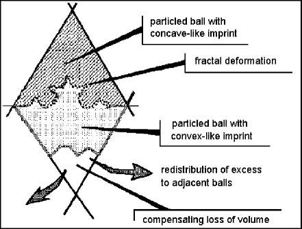
Figure 1: Schematic representation of the paired deformations produced by the collapse of a quantum of fractal deformations into a ball. One of the two complementary topologies could be called a positive charge and the other a negative one.

The progression of such structures in the degenerate space will generate several kinds of inerton cloud equivalent, depending on convexity trends ($\Xi$) and symmetry properties ($\Psi$) of the corresponding structures.

The properties generated by $\rm Q=\{\Xi,{\kern 1.0pt}\Psi\}$ will be called ”charge effects”.

3.3.3.2. Electric and magnetic charges. The motion of a particled ball in the space lattice exhibits some similarity with a cutwave which would be produced by a boat made with water. The shape of the waves depend on the shape of the moving object, as shown in Figure 2.

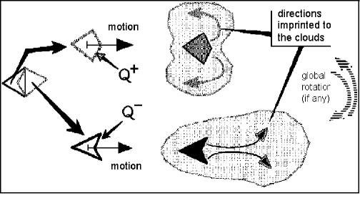
Figure 2: Changes imprinted in the shape of the inerton clouds by the shape of the particles deformations of symmetric type.

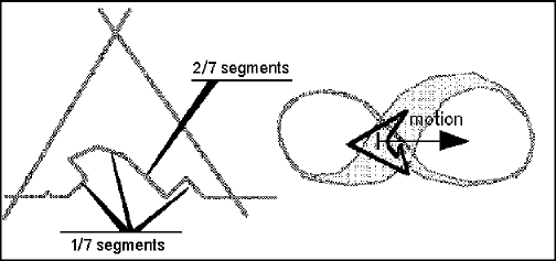
Figure 3: An asymmetric component in the deformation of a particle induces a torsion of the inerton cloud.
Note: The figure illustrates a initiator figure composed of seven subsegments of ratio (1/7) and two subsegments of ratio (2/7) of the modified side. Thus, the fractal is roughly depicted by $\rm 7\cdot(l/7){\kern 2.0pt}e+2\cdot(2/7){\kern 2.0pt}e=1$.

Component $\{\Xi\}$ of Q produces two kinds of inerton clouds (Figure 2), which can be identified with electric fields, since they depart from the ”neutral” inerton cloud by a symmetric kind of deformation. These shapes are complementary and can be associated in a oriented field, providing the corresponding area of the lattice with vectorial properties.

Component $\{\Psi\}$ appears when the fractal clusters are no longer symmetric in a massive particle. This case corresponds to well characterizable parametrizations. For instance, a sufficient condition is that the fractal quanta of masses have the following form, where at least some $\rm N_{{\kern 1.0pt}i}$ are odd numbers:

$$\rm(\Gamma)=\Big{(}\{N_{{\kern 1.0pt}i},{\kern 1.0pt}a_{{\kern 1.0pt}i},{\kern 1.0pt}\varrho_{{\kern 1.0pt}i}\}:{\kern 2.0pt}{\kern 2.0pt}{\mathop{\sum}_{i}}{\kern 2.0pt}{\underline{N}}_{{\kern 2.0pt}i}\cdot(\varrho_{{\kern 1.0pt}i})^{{\kern 0.5pt}e_{{\kern 0.5pt}i}}=1\Big{)}$$

In such cases, shown by Figure 3, the asymmetry will provide the cloud of inertons with an additional deformation represented by a torsion.

Neutrality may not be so simple. In a strict sense, it can be reflected by the absence of deformation. However, it can also be represented by symmetry and homogeneity of the distribution of convex and concave components simultaneously present on the same edges of particles, while the volume reduction associated to mass would remain fulfilled. The latter case would stand for a pseudo-neutrality worth to be taken in consideration. Figure 4 illustrates these features in a quasi-metaphoric sense.

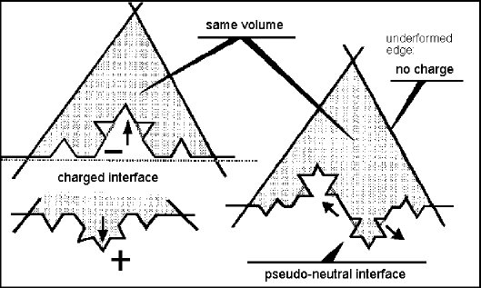
Figure 4: Illustration of canonical particles differing only by their charge. A strictly neutral edge would have no deformation. A charged edge can show cavities or protuberances.
Note: A pseudo-neutral interface would have the same quantity of cavities and protuberances and it would be in theory dissociable into two opposite charges.

3.3.4. Predicted expansion and the ”quintessence”

3.3.4.1. Introduction. Each time the distribution of degenerate deformations collapses into particled balls, there occurs a corresponding increase of volume of the surrounding balls, which compensates the reduction of volume in the particled cell. The motion of the particle can likely be provided by the reaction to the creation of this kind of ”anti-inerton cloud, which behaves in a opposite way than the resistance of the inerton cloud to the motion of the particle.

These increases of volume are then progressively scattered by transfer of the corresponding deformations to an expanding cloud of ”dilatation” quanta. This phenomenon operates a gain of space volume away of the particles: therefore, it represents a kind of force acting in a way opposite to the gravitation. This suggests two main corollaries.

3.3.4.2. Quintessence. The existence of a ”fifth cosmic element”, somewhat related with Einstein’s ”cosmological constant” has been thoroughly discussed (see Krauss, 1999; Börner, 2000; Ostriker and Steinhardt, 2001, etc. for review). In our model, this factor appears strictly in connection with the creation of matter from the degenerate lattice, which may stand for the cosmic form of a void. Its quantitative expression is directly correlated with the density of fractal deformations, that is of energy, and its range will be shown below to be of the long type. Basically, the above theorem of distribution shows that it appears independently of any previous presence of matter nor radiations. Last, it seems not to be braked by gravitational forces, since it appears as a by-product of the same event which produces gravity. All these points make this compensatory dilatation phenomenon a candidate for the ”quintessence”.

3.3.4.3. Space expansion. The transfer of elementary volumes released by the formation of massic particles occurs within the frame of the degenerate space, since it is processed in a nonfractal state, just for the compensation of lost volumes, without need for dimensional change. Call (a) such a element of volume: first, it is finite.

While the area of the iterated self-similar transform is theoretically infinite, its volume in 3-D sections is not. Therefore, while a part of the volume of the transformed cell is reduced by a finite value, the volume of surrounding cells is increased by a corresponding finite value. The homogeneity of the lattice is partly restored through progressive transfer of the additional volume to neighbor cells.

Remark 3.4. A degenerate ball constitutes a ”superparticle”.

Proof. The oscillations of an elementary cell have been considered by Krasnoholovets (1997; 2000) as the ”degenerate” state of space. It is a state without formation of a particle, though potentially able to provide particles upon proposition 3 and statement 3. One elementary ball thus constitutes the putative generator of particles, what has been called a ”superparticle” in previous attempts for unification of theories.

Remark 3.5. In any one Poincaré section, representing a timeless instantaneous state (an instans) of universe, the lattice of space is represented by a stacking of balls with nonidentical shape.

Conjecture 3.1. Elementary balls exhibit increasing volumes from the center to the periphery of a 3-D stacking.

Justifications. Three arguments concur to the same proposition.
(i) Oscillating deformations in excess in one cell can be partly compensated by transfer to neighboring balls, like an equivalent to the inerton cloud surrounding a particled ball. However, in central parts, the volume available is limited by the density of the stacking, and this limit is likely decreasing while going to the outer coats of the lattice. In a simple estimation, we denote by (a) the radius of the canonical (smallest) volume which can be transferred from a ball to another. Assuming that each cell forwards a volume (a) to another situated closer to the periphery, in the stacking, then the radius of a ball in the n^th coat is approximated by:

$$\rm r_{{\kern 1.0pt}n}=r_{{\kern 1.0pt}i}+(n-1){\kern 1.0pt}a$$

(ii) While the above considerations are valid for a particleless lattice, if the lattice is filled with particled balls, then there results a kind of pressure due to the inerton clouds. Hence, relation (4.2) is affected a corrective quantitative term to (a) and its distribution is determined by the distribution of particled balls in the considered space.
(iii) In contrast with the finiteness of volume to be compensatively distributed in the surrounding cells, the area of a particled cell is infinite, and the needed area cannot be compensated by a finite number of the surrounding cells. Thus an influence of any particle is likely to be found up to the most remote parts of the lattice.

The last two points will be further examined more in details in the third part of this study, through involvement of the concept of quantum of fractality in relation with mass of particled cells.

Corollary 3.2. Since elementary balls can be found at various scales, due to the quantic ratios which characterize the lattice, as shown above, this means that elementary particles are not of one unique size.

Corollary 3.3. Transfers of non fractal elementary volumes between balls are operated without dimensional increase.

Proof. At each given scale, the corresponding increments (a) are represented by similar topological features. In effect: following relation (3), we have for $\rm n=2$: $\rm r_{2}=r_{1}+a$, and for $\rm n=1$: $\rm r_{1}=r_{0}+(n-1){\kern 1.0pt}a=r_{0}$. Since then $\rm r_{0}=r_{2}-a$, $\rm r_{0}$ stands for a founding ball. Let $\rm r_{0}=$Ø, an empty set. Then, $\rm r_{2}=r_{0}+a$ can be represented by (Ø, {Ø}) where {Ø} is the frontier of ball r₂. The element {Ø} is what is exchangeable, and since it is a frontier, it has a dimension lower than the dimension of the interior, that is: $\rm dim(a)<dim(r)$. Thus exchanges do not modify the dimensionality of involved balls.

However, mass transfers from a particled cell to its surrounding degenerate balls involves a distribution of quanta of fractality through the concept of fractal decomposition described above.

Remark 3.6. Consequently, it may be considered that these exchanges apply to the frontiers of the balls, which will result in changes in the density of their internal structures. It is noteworthy that the density has been used as a probe for the identification of the packing of balls, though in this case only solid balls are considered (Hales, 2000). Otherwise, the adjunction of (a) to (r) may result in the reunion of two spaces having nonequal dimensions, which can result in a structure of the ”beaver space” type as described in Part 1.

Corollary 3.4. A measure on such a lattice space by using a scanning function as described in Part 1 will not scan the same components in elementary balls situated at various distances from its origin. Since there likely occurs an increase of the composition of balls from this origin, then the gauge will decrease with increasing distances: in effect, a larger set of scanned structures will appear at farther distances. Then, remote distances will be overestimated by a measure using a local gauge. This might account for the phenomenon known as the Doppler effect, in turn usually involving the Hubble constant. It should be noted here that the interpretation of the redshift has been matter of diverging treatments (e.g.: Hannon, 1998).

3.3.5. Towards a formalism to Big-Bang(s)

In Part 1 of this study, it has been proved:

(i) that the lattice existing from empty hyperset units provide a manifold of quantic scales represented by a set of defined integer ratios (Bounias and Krasnoholovets, 2002a) and

(ii) that there exists empty set units of various size, with integer vs.rational similarity ratios.

One universe $\rm U_{j}=\{\{S_{{\kern 1.0pt}i}\}_{i},{\perp}\}_{j}$, represented by one particular sequence of Poincaré sections selected through a particular combination rule is nothing but a manifold of organized empty set units, and since the lattice in which it is embedded is strictly fractal, the reunion of these empty set units is a higher scale empty set. Thus, $\rm U_{j}=$Ø_j.

Now, consider the part of the embedding lattice in which Ø_j owns just the size of a free ball. This ”over universe” denoted Ø_+j will behave like described through Proposition 1. The distribution collapse of degenerate balls of Ø_+j will result in the formation of a particle whose subparts contain potentially as many quanta of fractality as $\rm U_{j}$ contains massive objects. Thus, what represents a creation of a particle inside $\rm U_{j}$ is a primordial condensation of a ball into $\rm U_{j}$ inside $\rm U_{+j}$.

This suggests that such kinds of ”Big-Bangs” may have occurred, occur and will occur in at least denumerably many balls of the embedding lattice, without need for a ”outside” provision of energy.

However, these ”Big-Bangs” fulfill some conditions. In effect, it has been specified in Part 1 of this study that universe is definitely constructed in a specified space ($\rm W^{\omega})=\{X,\perp\}$ with set $\rm X\in\{X^{3}\cap X^{4}$) and combination rule ($\perp$) determining the choice of Si+1 from Si. Hence, relations between different universes and past-to-present successive universes can exist only through the same law ($\perp$).

4. Discussion and Conclusions

The law ($\perp$) proposed as the operator of the selection of successive Poincaré sections constituting a spacetime presents the interest, besides providing continuity of this spacetime, of keeping inert or low-moving structures (like mountains, landscapes, etc.) stable. Furthermore, it brings as a corollary that events will basically follow the shorter path between two steps, which is consistent with both the least action principle and the geodesic trajectory principle. This suggests that the kind of universe that we have described is consistent with our observable spacetime, even if our description of submicroscopic events, through the formalism of set theory extended to nonwellfounded sets (a consistent extension) may be considered in some sort as a metaphoric description.

The components of the {particle + inertons} system are likely inhomogeneous as topological balls do not need to be strictly spherical (the latter case is just a particular one).

Therefore, their coexistence in a single system representing the dual {wave/particle} system deserves special attention, since spin-related properties could reflect the eddy-like motion that inhomogeneity should impulse to the components and finally, in a resulting manner, to the system. Such properties have been described by Lin and OuYang (1980; 1998), Wu and Lin (2002), while Lin (1988) explored the compatibility of world exploration with the theoretical study of systems: these goals are well converging with our objective of mathematical exploration of an unknown world, as developed in Part 1 of this study.

The theoretical reasoning presented in this study, following the basis developed in Parts 1 and 2, sheds some light on the question of the hypothetic ”origins” of universe. In fact, there is no need for beginning nor for end. Even the expansion might not induce the consequences expressed through other approaches in terms of forever expansion and progressive immobilization, nor cyclic contraction and collapse. Our approach, basically founded on a formal justification of existence of ”something”, and then on corpuscular description and properties, turns to introduce some insights about cosmic scales and cosmic-size properties. Interestingly, Andreï Linde pioneeringly suggested that a ”Grand-Universe” could be composed of bubbles of universes that could form and disappear in various parts in an independent fashion. Though it was not primarily our aim to treat these questions, it turns out that the development of our model from defined startpoints comes to support Linde’s hypothesis.

Furthermore, the former hypothesis raised long ago by Feynman about particle trajectories which would be infinite and not derivable is consistent with our proposition that particles are distinguished from the degenerate space by a shift of dimensional properties, that is with a fractal organization.

The next part of this study will aim to examine more in detail what are the peculiarities of the various kinds of corpuscles predicted by our approach.

References

Bonaly, A., Bounias, M., 1995. ”The trace of time in Poincaré sections of topological spaces”, Physics Essays, Vol. 8, No. 2, pp. 236-44.

Börner, G., 2000. ”The infinitely large”, Pour La Science (Scientific American, French edition), Vol. 278, pp. 120-7.

Bounias, M., Bonaly, A., 1997. ”Some theorems on the empty set as necessary and sufficient for the primary topological axioms of physical existence”, Physics Essays, Vol. 10, No. 4, pp. 633-43.

Bounias, M., Krasnoholovets, V., 2003a. ”Scanning the structure of ill-known spaces: Part 1. Founding principles about mathematical constitution of space”, Kybernetes: The International Journal of Systems and Cybernetics, Vol. 32, No. 7/8, pp. 945-75. (Also physics/0211096.)

Bounias, M., Krasnoholovets, V., 2003b. ”Scanning the structure of ill-known spaces: Part 2. Principles of construction of physical space”, Kybernetes: The International Journal of Systems and Cybernetics, Vol. 32, No. 7/8, pp. 976-1004. (Also physics/0212004.)

Frizsh, H., 2000. ”The infinitely small in physics”, Pour La Science (Scientific American, French edition), Vol. 278, pp. 112-9.

Hannon, R.J., 1998. ”An alternative explanation of the cosmological redshift”, Physics Essays, Vol. 11, No. 4, pp. 576-8.

Hales, T.C., 2000. ”Cannonballs and honeycombs”, Notices of the AMS, Vol. 47, No. 4, pp. 440-9.

Krasnoholovets, V., 1997. ”Motion of a relativistic particle and the vacuum”, Physics Essays, Vol. 10, No. 3, pp. 407-16. (Also quant-ph/9903077).

Krasnoholovets, V., 2001. ”On the way to submicroscopic description of nature”, Indian Journal of Theoretical Physics, Vol. 49, No. 2, pp. 81-95. (Also quant-ph/9908042).

Krauss, L., 1999. ”Antigravity”, Pour La Science (Scientific American, French edition), Vol. 257, pp. 42-9.

Lin, Y., OuYang, S.C., 1996. ”Exploration of the mystery of nonlinearity”, Research of Natural Dialectics, Vol. 12-13, pp. 34-7.

Lin, Y., 1988. ”Can the world be studied in the viewpoint of systems?”, Math. Comput. Modeling, Vol. 11, pp. 738-42.

Lin, Y., OuYang, S.C., 1998. ”Invisible Tao and realistic nonlinearity propositions”. Kybernetes: The International Journal of Systems and Cybernetics, Vol. 27, pp. 809-22.

Ostriker, J., Steinhardt, P., 2001. ”The fifth cosmic element”. Pour La Science (Scientific American, French edition), Vol. 281, pp. 44-53.

Rüegg A., 1985. Probabilities and Statistics, Presses Polytechniques Romandes, Mausanne, Switzerland, pp. 52-87.

Wang, L., Caldwell, R., Ostriker, J., Steinhardt, P., 2000. ”Cosmic concordance and quintessence”, Astrophysical Journal, Vol. 530, No. 1, pp. 17-35.

Wu, Y., Lin, Y., (2002). ”Beyond nonstructural quantitative analysis”, in Blown ups, spinning currents and modern science, World Scientific, New Jersey, London, p. 324.

Further reading

Caldwell, R., Dave, R., Steinhardt, P., 1998. ”Cosmological imprint of an energy component with general equation of state”, Phys. Rev. Lett., Vol. 80, No. 8, pp. 1582-5.

Krauss, L., 1998. ”The end of age problem, and the case for a cosmological constant revisited”, Astrophysical Journal, Vol. 501, No. 2, 461-6.

Schwartz, L., 1997. Un mathématicien aux prises avec le siècle, Odile Jacob, Paris, p. 250.