Obervational Model for Microarcsecond Astrometry with
the Space Interferometry Mission

Abstract

The Space Interferometry Mission (SIM) is a space-based long-baseline optical interferometer for precision astrometry. One of the primary objectives of the SIM instrument is to accurately determine the directions to a grid of stars, together with their proper motions and parallaxes, improving a priori knowledge by nearly three orders of magnitude. The basic astrometric observable of the instrument is the pathlength delay, a measurement made by a combination of internal metrology measurements that determine the distance the starlight travels through the two arms of the interferometer and a measurement of the white light stellar fringe to find the point of equal pathlength. Because this operation requires a non–negligible integration time to accurately measure the stellar fringe position, the interferometer baseline vector is not stationary over this time period, as its absolute length and orientation are time–varying. This conflicts with the consistency condition necessary for extracting the astrometric parameters which requires a stationary baseline vector. This paper addresses how the time-varying baseline is “regularized” so that it may act as a single baseline vector for multiple stars, and thereby establishing the fundamental operation of the instrument.

Keywords: SIM, metrology, pathlength feedforward, astrometry, modeling

1 INTRODUCTION

SIM is designed as a space-based 10-m baseline Michelson optical interferometer operating in the visible waveband. This mission will open up many areas of astrophysics, via astrometry with unprecedented accuracy. Over a narrow field of view SIM is expected to achieve a mission accuracy of 1 $\mu$as. In this mode SIM will search for planetary companions to nearby stars by detecting the astrometric “wobble” relative to a nearby ($\leq 1^{\circ}$) reference star. In its wide-angle mode, SIM will be capable to provide a 4 $\mu$as  precision absolute position measurements of stars, with parallaxes to comparable accuracy, at the end of a 5-year mission. The expected proper motion accuracy is around 4 $\mu$as/yr, corresponding to a transverse velocity of 10 m/s at a distance of 1 kpc.[1]

The SIM instrument does not directly measure the angular separation between stars, but the projection of each star direction vector onto the interferometer baseline by measuring the pathlength delay of starlight as it passes through the two arms of the interferometer. The delay measurement is made by a combination of internal metrology measurements to determine the distance the starlight travels through each arm, and a measurement of the central white light fringe to determine the point of equal pathlength.

SIM surveys the sky in units called tiles. A tile is defined as a sequence of measured delays corresponding to multiple objects all made by a single baseline vector $\vec{b}$ and central pointing of the instrument – that is, all the measurements in a tile are from objects that are within a single astrometric FOR (field of regard of the instrument), which is approximately $15^{\circ}\times 15^{\circ}$. The existence of a single baseline vector insures that the system of equations developed from the observations to extract the astrometric parameters is not underdetermined. However, the collection of such a measurement set with a single interferometer is actually impossible, as the data collection on a sequence of objects takes finite time, over which both the baseline length and orientation do not remain constant.

This paper describes the fundamental steps of how the on–board instrumentation of external metrology and auxiliary guide interferometers are used to reconstruct the baseline vector sufficiently accurately so that it can effectively be modeled as a single vector over the period of a tile observation. This process has been previously referred to as the regularization of the baseline [2]. The notion of the regularized baseline has been used extensively in a number of grid simulation studies that plan observation sequences, predict mission accuracy, and determine sensitivities to various instrument parameters [2, 3, 4].

The process of reconstructing the baseline vector when implemented onboard in real–time is termed pathlength feedforward, and is a critical component to the operation of the interferometer. Because many of the astrometric targets will be very dim, it is not possible for the science interferometer to track the fringes and compensate for optical pathlength difference variations in real time using the dim target as the signal. As a result the fringes associated with the science target will be washed out due to uncontrolled motions of the instrument. The adopted solution in these cases is to use precise attitude information obtained from the two guide interferometers and construct a delay tracking signal that will be fed to the science interferometer’s delay line in an open loop fashion. This aspect of the baseline regularization process will be covered in some detail. An overview of the mission and several of the major subsystems of the instrument can be found in references [5, 6, 7, 8]

2 Astrometry with SIM

SIM is designed to measure the pathlength delay between the two arms of the interferometer. The instantaneous delay value is given formally by the interferometer astrometric equation: [4]

$$d(t)=\big{(}\vec{b}(t)\cdot\vec{s}\big{)}+k+\eta(t),$$ (1)

where $d$ is the external optical pathlength delay synthesized by a combination of internal metrology and white light fringe estimation, $\vec{s}$ is the normal to the wavefront of the starlight (the unit 3-vector to the observed object), $\vec{b}$ is the baseline 3-vector, $k$ is a so-called constant (or calibration) term that represents possible optical path differences between the light collected from the target object and the internal metrology, and $\eta(t)$ is the noise in the measurement.

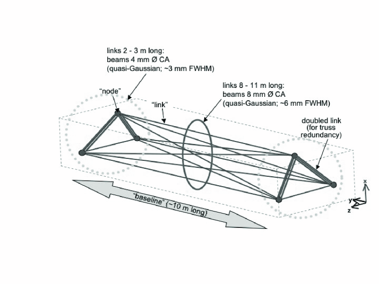
Figure 1: SIM External metrology design

Because of limitations imposed by the optical throughput of the system and the brightness of the observed objects several seconds of integration time are necessary to bring the average white light fringe estimate to the required accuracy. Thus, the actual instrument measurement is the following:

$$\langle d_{i}\rangle=\big{(}\vec{s}_{i}\cdot\langle\vec{b}\rangle\big{)}+k+\eta_{i},$$ (2)

where $\langle d_{i}\rangle$ is the average measured external delay obtained from internal metrology measurements and white light fringe estimation, $\langle\vec{b}\rangle$ is the average baseline vector over the period of the observation, and $\eta_{i}$ is the measurement noise.

The fundamental objective of the instrument is to make these delay measurements so that the astrometric parameters of position, proper motion, and parallax can be ascertained for the stars that are observed. Focusing just on the problem of estimating stellar positions, the astrometry problem is to determine the vector $\vec{s}$ in Eq. (2) above. However, all of the quantities above on the right must be treated as unknown because of the $\mu$as level precision requirements of the instrument. (The Hipparcos catalogue has an accuracy on the order of several mas for stellar positions, while standard attitude determination and alignment systems on spacecraft can determine the baseline vector to the order of an arcsec.) SIM circumvents this difficulty by observing multiple stars, $\{s_{i}\}$, within its field of regard so that the observation equations can be modeled as

$$d_{i}=s_{i}\cdot b+k+\eta_{i},\qquad i=1,...,N.$$ (3)

The critical assumption here is that there is a single baseline vector, albeit unknown, that needs to be solved for as well as a single constant term. Thus, Eq. (3) consists of $N$ equations with $2N+4$ unknowns. If a new baseline orientation is used to observe the same set of stars, an additional $N$ equations are obtained, but only at the expense of 4 additional unknowns necessary to determine the new baseline vector and constant term. It is evident with more observations the system of equations eventually becomes overdetermined so that the stellar positions can be resolved. Applying this idea to a set of tiles that covers the entire celestial sphere is the kernel of SIM’s strategy to perform wide angle astrometry.

The observable in (2) is the average delay measurement made by the interferometer. Considerable analysis, simulation and technology development and validation has been devoted to the problems of precision white light fringe estimation and metrology that are used to synthesize this observable.[9, 10, 11, 12, 13, 14, 15] The focus of this paper is to show that the model equations Eq. (3) are actually consistent with the data that is collected by the instrument. To see where a potential conflict may arise, observe that because the baseline vector is time–varying, the average position over the integration period changes from observation to observation. The resulting model over a tile is

$$\langle d_{i}\rangle=s_{i}\cdot\langle b_{i}\rangle+k,\quad i=1,...,N.$$ (4)

The difficulty now is that there is a different (unknown) average baseline for each star; violating the assumption made in (3).

In principle SIM solves this problem by using guide interferometers and external metrology to track the baseline vector during the observations. The details of this process will be developed over the next two sections. Here will give the overview of how this is done, specifically with respect to overcoming the difficulty posed in (4).

SIM uses two auxiliary guide interferometers that lock on bright “guide” stars ($\vec{g}_{1}$, $\vec{g}_{2}$), thereby keeping track of the directions to these stars, and hence also of the rigid-body motion of the instrument. The third interferometer switches between the science targets ($s_{\tt 1}$, $s_{\tt 2}$, $\cdots$), measuring the projected angles between the targets and the interferometer baseline vector. An external metrology system keeps track of the flexible-body motions of the instrument by measuring changes in the baseline vectors of the three interferometers in a local frame, or equivalently, determining their relative orientations.

Because the three interferometer baselines are not collinear, to complete the characterization of the rigid body behavior of the instrument a third inertial measurement is required. This measurement is termed the “roll” measurement. In the ideal case we show that the SIM instrumentation is sufficient in the sense that in the absence of measurement errors and a priori parameter errors, the collection of measurements made by the guide interferometers, the roll measurement, the external metrology measurements together with the a priori parameter data consisting of the positions of the guide stars, the initial guide and science baseline vectors in the local frame, uniquely determine the baseline vector of the science interferometer in inertial space.

When this is the case the vector $\langle b_{i}\rangle$ in (4) is known for all $i$. In reality there are both measurement errors and a priori parameter errors so it can never be assumed that the $\langle b_{i}\rangle$ are known. For any parameter vector $p$, let $b(t;p)$ be the estimate of the baseline vector using this parameter vector. In the absence of measurement error the sufficiency of the SIM instrumentation is embodied in the statement that $b(t)=b(t;p_{0})$ where $p_{0}$ is the true parameter vector. Let $p$ denote the a priori parameter vector and write

$$\delta\vec{b}(t)=\vec{b}(t;p_{0})-\vec{b}(t;p).$$ (5)

In Section 5 we show that for $|p-p_{0}|$ sufficiently small

$$\delta\vec{b}(t)=\delta\vec{b}^{0}+\vec{\epsilon}(t),$$ (6)

where $\delta b_{0}$ is a constant vector (so long as the guide interferometers are locked on the guide stars) and $|\epsilon(t)|$ is a residual variation that contributes a delay error much less than the magnitude of the measurement noise $\eta_{i}$ and can be ignored in the analysis.

Now we may write the instantaneous delay equation as

$$d_{i}(t) = \vec{s}_{i}\cdot\vec{b}(t;p)+\vec{s}_{i}\cdot\vec{\delta b}(t)+k$$ (7)

$$= \vec{s}_{i}\cdot\vec{b}(t;p)+\vec{s}_{i}\cdot\vec{\delta b}^{0}+\vec{s}_{i}\cdot\vec{\epsilon}(t)+k.$$

Let $\vec{s}_{i}{}^{0}$ denote the a priori estimate of the position so that $\vec{s}_{i}=\vec{s}_{i}{}^{0}+\vec{\delta s_{i}}$, where $\vec{\delta s_{i}}$ is the correction vector that is sought. Thus, after averaging

$$\langle d_{i}(t)\rangle-\vec{s}_{i}{}^{0}\cdot\langle\vec{b}(t;p)\rangle=\vec{\delta s_{i}{}^{0}}\cdot\langle\vec{b}(t;p)\rangle+\vec{s}_{i}{}^{0}\cdot\langle\delta\vec{b}^{0}\rangle+\vec{s}_{i}{}^{0}\cdot\langle\epsilon(t)\rangle+k.$$ (8)

The quantity on the left is termed the “regularized delay” and is the quantity that is synthesized from the SIM instrumentation. And since $\vec{b}(t;p)$ is known and the contribution of the term containing $\epsilon(t)$ can be ignored, the unknowns are the corrections to the science star positions and the correction to the baseline vector which is now a single constant vector over the entire tile. In this sense the idealized model equations in (3) are correct.

2.1 The ideal instrument measurements

We will now get into the details of how $\langle\vec{b}\rangle$ is obtained from the measurements and a priori data. For this purpose it suffices to treat SIM as a set of fiducials, $\vec{X}_{1},...,\vec{X}_{N},~{}\vec{X}_{i}\in{\bf R^{3}}$. (Here ${\bf R^{3}}$ denotes Euclidean 3–space.) In the SIM reference design, shown in Figure 1, there are a total of six fiducials, and in a spacecraft local frame their coordinates are collected in the matrix $\vec{X}_{\tt fid}$ (with units in meters):

$$\vec{X}_{\tt fid}=\left[\matrix{0&0&0\cr 1.4&.55&-1.4\cr 0&0&-2.8\cr 0&10&-2.8\cr 1.4&9.45&-1.4\cr 0&10&0\cr}\right].$$ (9)

The $i^{th}$ row of $X_{\tt fid}$ defines the coordinates of $\vec{X}_{i}$.

The science interferometer baseline vector $\vec{b}_{s}$ is defined as

$$\vec{b}_{s}=\vec{X}_{\tt fid}(6,:)-\vec{X}_{\tt fid}(1,:).$$ (10)

The auxiliary science baseline vector is defined by fiducials 3 and 4. The guide interferometer baseline vector $\vec{b}_{g}$ is defined

$$\vec{b}_{g}=\vec{X}_{\tt fid}(5,:)-\vec{X}_{\tt fid}(2,:),$$ (11)

and the “roll” vector is

$$\vec{\tau}=\vec{X}_{\tt fid}(2,:)-\vec{X}_{\tt fid}(1,:).$$ (12)

For any pair of vectors in ${\bf R^{3}}$, say $\vec{W}_{i}$ and $\vec{W}_{j}$, the vector $\vec{W}_{ij}$ will denote the difference $\vec{W}_{ij}=\vec{W}_{i}-\vec{W}_{j}$. Thus, for example $\vec{b}_{s}=\vec{X}_{16}$. Our interests center around the evolution of the fiducials $\vec{X}_{i}(t)$ over a time period $t_{0}\leq t\leq T$, where $t=t_{0}$ denotes the beginning of an observation of a tile and $t=T$ is the time of completion. The problem is solved using the on–board optical sensing systems that include the external metrology system, the guide star interferometers, and the roll estimator. The signals from these systems are briefly described next.

In the SIM reference design relative distance measurements are made between each pair of fiducials except for the direct link connecting the active science interferometer fiducials. The observed variables associated with the external metrology system are

$$\ell_{ij}(t)=|\vec{X}_{ij}(t)|-|\vec{X}_{ij}(t_{0})|,\qquad j>i,i=1,...5,~{}~{}{\rm excluding}~{}(i=1\,\,\&\,\,j=6).$$ (13)

These measurements are relative distance measurements, and (13) is valid for any choice of coordinate frame. Thus, $\vec{b}_{\tt s}$ is determined in the local frame from (10). The problem is to find $\vec{b}_{\tt s}$ in the inertial frame. This connection is made with the guide interferometers.

SIM uses a pair of guide stars to produce two independent delay measurements per observation:

$$d_{\tt gA}=(\vec{g}_{\tt A}\cdot\vec{b}_{\tt gA})+k_{\tt gA},$$ (14)

where $\vec{g}_{\tt A}$ is the position vector to guide star $A$, with $A\in(1,2)$.

The roll estimator produces a “measurement” similar to the guide interferometers. We designate a guide telescope for use as part of the roll estimation scheme, and let $\vec{n}$ denote the line–of–sight vector of this telescope. Next we introduce a fiducial rigidly attached to the telescope which is also measured by the external metrology system. Let $\vec{\tau}$ denote the vector connecting this fiducial with the fiducial mounted on the chosen guide telescope. The rigidity assumption is that

$$\kappa=(\vec{n}\cdot\vec{\tau})$$ (15)

where $\kappa$ is constant for all values of $\vec{n}$ and $\vec{\tau}$ over the period of a tile observation.

2.2 The logic of SIM astrometric observations

Now we will describe how (13)–(15) are used to characterize the evolution of $\vec{b}_{\tt s}$ in the inertial frame.

First let us see what can be learned from the observations in (13). Set $\vec{X}=(\vec{X}_{1},...,\vec{X}_{N})$, and define $F(\vec{X})$ as the function with components $F_{ij}(\vec{X})$

$$F_{ij}(\vec{X})=|\vec{X}_{ij}(t)|-|\vec{X}_{ij}(t_{0})|,\qquad j>i;\quad i=1,...5,\quad i\not=1\quad\&\quad j\not=6.$$ (16)

We seek the solution to the system of equations

$$F(\vec{X})=\ell,\quad\ell=(\ell_{ij}).$$ (17)

The first thing to note is that if $\hat{U}$ is a rotation matrix acting on vectors in ${\bf R^{3}}$, and if $\vec{\xi}\in{\bf R^{3}}$, then

$$F(\vec{X})=F(\vec{Y}),\quad\hbox{where}\quad\vec{X}=(\vec{X}_{1},...,\vec{X}_{N}),\quad\vec{Y}=(\hat{U}\vec{X}_{1}+\vec{\xi},...,\hat{U}\vec{X}_{N}+\vec{\xi})$$ (18)

since

$$|\hat{U}\vec{X}_{i}+\vec{\xi}-(\hat{U}\vec{X}_{j}+\vec{\xi})|=|\hat{U}\vec{X}_{ij}|=|\vec{X}_{ij}|.$$ (19)

The final equality in (19) follows because $\hat{U}$ is orthogonal, and hence, preserves norms. Importantly the converse of (18) also holds: Property 1: If $F(\vec{X})=F(\vec{Y})$ for some pair $\vec{X}$ and $\vec{Y}$ (in a small neighborhood $N$ of $\vec{X}_{0}$), then there exists a rotation matrix $\hat{U}$ and 3–vector $\vec{\xi}$ such that $\vec{Y}_{i}=\hat{U}\vec{X}_{i}+\vec{\xi}$ for all $i$. This is the fundamental result which links the local and inertial frames. The linear justification of this principle is that since $F(\vec{X})=F(\vec{Y})$ and to first order $F(\vec{Y})=F(\vec{X})+F^{\prime}(\vec{X})(\vec{Y}-\vec{X}),$ it follows that $\vec{Y}-\vec{X}$ must be in the kernel of $F^{\prime}(\vec{X})$, which can be characterized as the rigid body motions of the fiducial system. It is not difficult to extend the linear argument to the full result.

Let $\vec{X}$ denote the vector of fiducial positions in inertial coordinates. Then (in the absence of noise) $\vec{X}$ solves (17). If $\vec{X}^{\tt loc}$ is a solution to (17) computed in a local spacecraft coordinate frame, then Property 1 states that there is a rotation matrix $\hat{U}$ such that

$$\vec{X}_{ij}=\hat{U}\vec{X}_{ij}^{\tt\,loc}$$ (20)

for every pair of fiducials $\vec{X}_{i}$ and $\vec{X}_{j}$. Thus the matrix $\hat{U}$ is the transformation between the local and inertial coordinate frames. And since the science baseline vector $\vec{b}_{\tt s}$ is known in local coordinates from external metrology measurements, the problem of determining $\vec{b}_{\tt s}$ in inertial coordinates is solved once we obtain $\hat{U}$, viz.

$$\vec{b}_{\tt s}=\hat{U}\,\vec{b}_{\tt s}^{\tt\,loc}.$$ (21)

The equations for obtaining $\hat{U}$ are provided by the guide interferometer measurements and the roll estimator. The guide measurements may be written as

$$d_{\tt gA}=(\vec{g}_{\tt A}\cdot\hat{U}\,\vec{b}_{\tt g}^{\tt\,loc})+k_{\tt gA},$$ (22)

with $\vec{b}_{\tt g}^{\tt\,loc}$ assumed known from external metrology data. The third equation needed to determine $\hat{U}$ is provided by the roll estimator, which has the form from (15)

$$\kappa=(\vec{n}\cdot\vec{\tau})=(\vec{n}\cdot\hat{U}\vec{\tau}^{{\tt\,loc}}),$$ (23)

where $\vec{n}$, $\kappa$ and $\vec{\tau}^{\tt loc}$ are all known. We now have 3 equations with which to determine $\hat{U}$. (The set of orthogonal matrices live in a space of three dimensions, so three non–redundant equations are sufficient.) Note that the roll estimator equation has essentially the same form as the guide equation. The correspondences are that the guide measurement is replaced by a constant value using the rigidity assumption of the structure connecting the fiducials used for roll, the inertial position of the guide star is replaced with the inertial line of sight vector of the telescope, and the guide interferometer baseline vector is replaced with roll vector connecting the two fiducials.

3 Solving the baseline vector equations

As described above, there are two components to the problem of determining $\vec{b}(t;p)$. The first part inverts the 1–D external metrology measurements into position vectors computed in the spacecraft local frame for all of the fiducials. The second part uses the guide interferometer measurements together with the roll estimator equation to determine the transformation between the local frame and the inertial frame.

3.1 Inverting the external metrology measurements

Because in general the system of external metrology equations Eq. (17) is overdetermined, the estimate of the fiducial positions $\vec{X}_{i}$ is derived from the solution to the nonlinear least squares problem

$$\min_{X}|F(\vec{X})-\ell|^{2},$$ (24)

where $\ell$ is the vector with components $\ell_{ij}$. In the case of the reference design, $\ell$ is a 14–vector comprised of links between every pair of the six fiducials of the external metrology subsystem, except for the one pair that is a direct link between the fiducials of the active science interferometer baseline. Let $F^{\prime}$ denote the differential of the function $F$ at $\vec{X}^{0}$. The rows of $F^{\prime}$ are constructed from the gradients of the functions $F_{ij}$. These gradients are easily calculated analytically as

$$\nabla F_{ij}(\vec{X}_{0})=[0_{1,3(i-1)},~{}\frac{(\vec{X}^{0}_{j}-\vec{X}^{0}_{i})^{T}}{|\vec{X}^{0}_{j}-\vec{X}^{0}_{i}|},~{}0_{1,3(j-i-1)},~{}-\frac{(\vec{X}^{0}_{j}-\vec{X}^{0}_{i})^{T}}{|\vec{X}^{0}_{j}-\vec{X}^{0}_{i}|},~{}0_{1,3(N-j)}],$$ (25)

where $0_{s,t}$ is the zero matrix with $s$ rows and $t$ columns. Thus $F^{\prime}$ is a $14\times 18$ matrix corresponding to the 14 metrology measurements and 18 coordinates representing the 6 fiducial positions. Let $F^{\prime{\dagger}}$ denote the pseudoinverse of the differential of $F$ at $\vec{X}^{0}$. (The pseudoinverse only needs to be calculated once at the beginning of the tile.) Then the iteration scheme beginning with $\vec{X}^{0}=(\vec{X}_{1}^{0},...,\vec{X}_{N}^{0})$,

$$\vec{X}^{k}=\vec{X}^{k-1}+F^{\prime{\dagger}}[\ell-F(\vec{X}^{k-1})],$$ (26)

can be shown to converge to the unique solution of (24) using a Gauss-Newton convergence argument. This solution is contained in a ball of radius $2|F^{{\dagger}}l|$ about $\vec{X}_{0}$ and an $O(|\ell|^{3})$ error is incurred if the iteration is stopped at $k=2$; which is sufficient for both SIM requirements as the constraints on the magnitude of the flexible body motion of the fiducials leads to $|\ell|\approx 10^{-5}$m. The use of the pseudoinverse in (26) is equivalent to constraining certain linear combinations of fiducial positions to remove the rigid body motions of the system.

3.2 The attitude equations

The second part of the algorithm for estimating $\vec{b}(t)$ requires solving for the attitude. The three equations for obtaining the transformation, $\hat{U}$, between the local and inertial frames are provided by the guide interferometer and the roll estimator equations.

$\hat{U}$ can be parameterized in several ways. We will make use of the fact that there is a skew–symmetric matrix $\hat{S}$ such that $\hat{U}=\exp(\hat{S})$ so that $\hat{U}$ has the series expansion

$$\hat{U}=\hat{I}+\hat{S}+\hat{S}^{2}/2!+\hat{S}^{3}/3!+....$$ (27)

We will also use the 1–1 correspondence between the set of skew symmetric matrices and 3–vectors via the mapping $\vec{\omega}\rightarrow\hat{S}(\vec{\omega})$,

$$\hat{S}(\vec{\omega})=\left[\matrix{0&-\omega_{3}&\omega_{2}\cr\omega_{3}&0&-\omega_{1}\cr-\omega_{2}&\omega_{1}&0\cr}\right],\quad\vec{\omega}=(\omega_{1},~{}\omega_{2},~{}\omega_{3}).$$ (28)

Without loss of generality we may assume that $\hat{U}\approx\hat{I}$ because of on–board attitude knowledge. The quadratic approximation to (22)–(23) using (27) and (28) is

$$T_{\tt ext}\vec{\omega}+G_{\tt ext}(\vec{\omega})=y,$$ (29)

where,

$$T_{\tt ext}=\left[\matrix{\vec{\tau}^{\tt loc}\times\vec{n}\cr T\cr}\right],\qquad T=\left[\matrix{\vec{b}_{g}^{\tt loc}\times\vec{g}_{1}\cr\vec{b}_{g}^{\tt loc}\times\vec{g}_{2}\cr}\right],$$ (30)

$$G_{\tt ext}(\vec{\omega})=\left[\matrix{0\cr G(\vec{\omega})\cr}\right],\qquad G(\vec{\omega})=-{1\over 2}\left[\matrix{\langle\vec{\omega}\times\vec{g}_{1},\vec{\omega}\times\vec{b}_{g}^{\tt loc}\rangle\cr\langle\vec{\omega}\times\vec{g}_{2},\vec{\omega}\times\vec{b}_{g}^{\tt loc}\rangle\cr}\right],$$ (31)

and

$$y=\left[\matrix{\kappa-\vec{n}\cdot\vec{\tau}^{\tt loc}\cr d_{g1}-\vec{g}_{1}\cdot\vec{b}_{g}^{\tt loc}\cr d_{g2}-\vec{g}_{2}\cdot\vec{b}_{g}^{\tt loc}\cr}\right].$$ (32)

It can be shown that the solution to (29) produces an error of $O(|\vec{\omega}|^{4})$ in determining $\hat{U}$. (This is less than a $10^{-15}$ rad error for 20 arcsec of motion of the instrument.) Without going into the details of the proof of this result here, we just remark that it hinges on the simple observation that for any skew symmetric matrix $\hat{S}$, the distance from $\hat{I}+\hat{S}+\hat{S}^{2}/2$ to an orthogonal matrix is $|O(\hat{S}^{4})|$. And this follows by noting that

$$(\hat{I}+\hat{S}+\hat{S}^{2}/2)(I+\hat{S}+\hat{S}^{2}/2)^{T} = \hat{I}+\hat{S}+\hat{S}^{T}+\hat{S}\hat{S}^{T}+\hat{S}^{2}/2+(\hat{S}^{2})^{T}/2+$$ (33)

$$+~{}\hat{S}(\hat{S}^{2})^{T}/2+\hat{S}^{2}\hat{S}^{T}/2+\hat{S}^{2}(\hat{S}^{2})^{T}/4=$$

$$= I+\hat{S}^{4}/4,$$

where $\hat{I}$ denotes the identity matrix and we have used $\hat{S}^{T}=-\hat{S}$ and $(\hat{S}^{2})^{T}=\hat{S}^{2}$. (Recall that a matrix $\hat{X}$ is orthogonal if $\hat{X}\hat{X}^{T}=\hat{I}$.)

Rewriting (29) as

$$\vec{\omega}=T_{\tt ext}^{-1}y-T_{\tt ext}^{-1}G_{\tt ext}(\vec{\omega}),$$ (34)

the solution can be obtained by a fixed point iteration on the mapping defined above on the right:

$$\vec{\omega}^{k}=T_{\tt ext}^{-1}y-T_{\tt ext}^{-1}G_{\tt ext}(\vec{\omega}^{k-1}),\quad\vec{\omega}_{0}=T_{\tt ext}^{-1}y;$$ (35)

with error estimate

$$|\vec{\omega}^{k}-\vec{\omega}|\leq|T_{\tt ext}^{-1}y|^{k+1}.$$ (36)

A standard contraction mapping argument can be used to establish this result. The estimated baseline in inertial space is then realized as

$$\vec{b}_{s}=\vec{b}_{s}^{\tt loc}+\vec{\omega}\times\vec{b}_{s}^{\tt loc}+{1\over 2}\vec{\omega}\times(\vec{\omega}\times\vec{b}_{s}^{\tt loc}),$$ (37)

where $\vec{b}_{s}^{\tt loc}$ is determined from (26), and $\vec{\omega}$ is obtained from the iteration in (35).

To simplify matters a little for the error analysis that will be performed in Section 5, we define $\vec{\omega}_{I}$ as the starting value in (35):

$$\vec{\omega}_{I}=T_{\tt ext}^{-1}y,$$ (38)

and $\vec{\omega}_{II}$ as the first iterate:

$$\vec{\omega}_{II}=\vec{\omega}_{I}-T_{\tt ext}^{-1}G_{\tt ext}(\vec{\omega_{I}}).$$ (39)

Because our estimates will carry through second order, the science baseline estimate we use is

$$\vec{b}_{s}=\vec{b}_{s}^{\tt loc}+\vec{\omega}_{II}\times\vec{b}_{s}^{\tt loc}+{1\over 2}\vec{\omega}_{I}\times(\vec{\omega}_{I}\times\vec{b}_{s}^{\tt loc}).$$ (40)

This second order approximation accommodates flexible fiducial motions on the order of tens of microns in the inversion of the external measurements and rigid body motions of 100 $\mu$rad in the attitude equations. These are both significantly larger than SIM requirements. As an example of these approximations, the plots in Figures 2 and 3 show induced motion of this magnitude in the system. The $x$ and $z$ axis motion shown are due to large (20 as) sinusoid motion of the baseline, while the $y$ axis motion is due mostly to flexible body motion superimposed on the rigid body displacement. Figure 4 shows the error in the estimated baseline components using the quadratic model. It is seen that these errors are sub–picometer, as the error analysis predicts. These methods could of course accommodate a larger range of motion at the expense of utilizing more iterations in the solution of the external metrology and attitude equations. A mission level simulation capability that incorporates these equations and a number of instrument models is under development.[16]

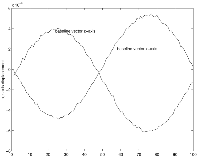
Figure 2: x and z baseline displacement vector components due to rigid body motion

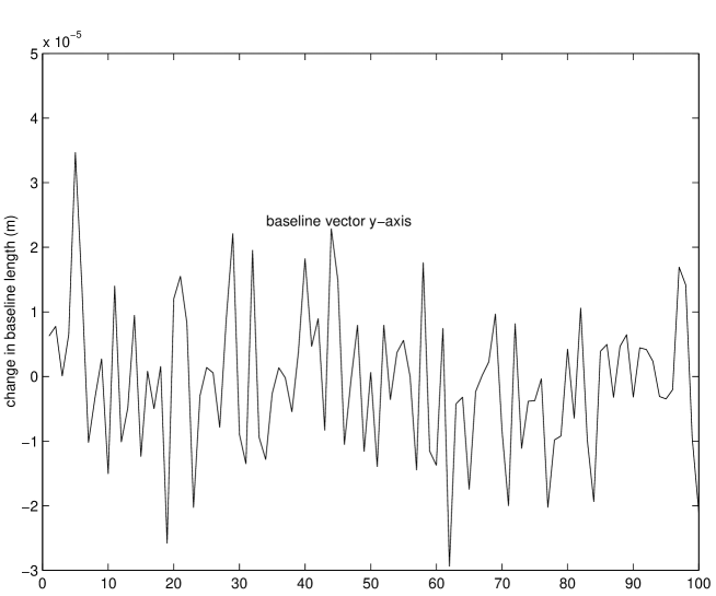
Figure 3: y baseline displacement vector component due to flex body motion

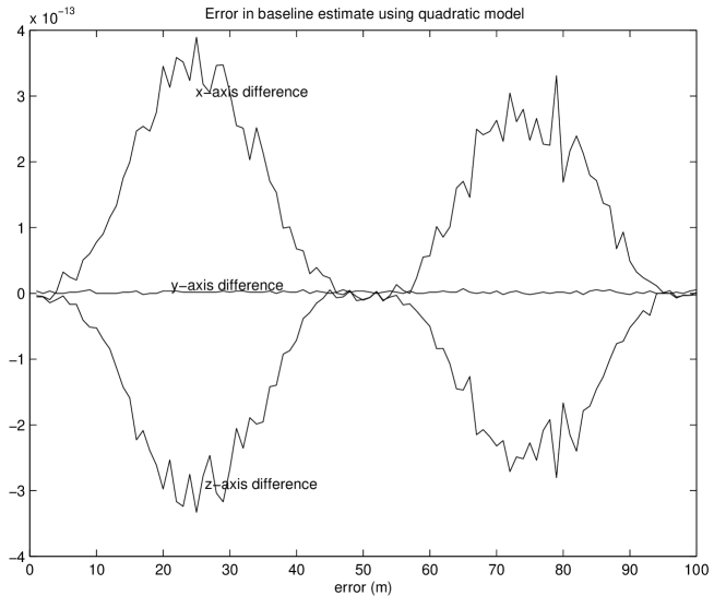
Figure 4: Error in baseline vector estimate due to quadratic approximation

4 A Geometric Interpretation

The solution to the set of non-linear equations that governs the evolution of the baseline vector has a geometric interpretation that will be discussed here. To facilitate this we introduce the baseline strain parameter $\epsilon$

$$\epsilon(t)=\frac{b(t)-b(t_{0})}{b(t_{0})}$$ (41)

which we expect to be $\sim\mu$rad because the change in the baseline length will be on the order of 10 $\mu$m.

Again retaining terms through second order in $\vec{\omega}(t)$, we parameterize the instantaneous interferometer baseline, $\vec{b}(t)$, as follows:

$$\vec{b}(t)=b(t_{0})\Big{(}1+\epsilon(t)\Big{)}\Big{(}\vec{n}(t_{0})+[\vec{\omega}(t)\times\vec{n}(t_{0})]+\frac{1}{2!}[\vec{\omega}(t)\times[\vec{\omega}(t)\times\vec{n}(t_{0})]]+{\cal O}\big{(}\omega^{3}\big{)}\Big{)},\hskip 20.0pt$$ (42)

where $b(t_{0})$, $\vec{n}(t_{0})$ are the initial baseline length and orientations of the guide interferometer; $\epsilon(t)=\Delta b(t)/b(t_{0})$ is the time-varying readings of the external metrology; $\vec{\omega}(t)$ is the vector of small attitude changes in the baseline orientation for the interferometer, $\vec{\omega}(t_{0})\equiv 0;$ and $[\vec{a}\times\vec{b}]$ denotes the cross vector product of vectors $\vec{a}$ and $\vec{b}$.

4.1 Science Interferometer Delay Equation

The expression (42) allows us to write the delays for all three interferometers. Thus, to second order in $\vec{\omega}$ one obtains the following expressions for the time-varying delays of the science and the two guide interferometers:

$$d_{\tt s}(t) \equiv k_{\tt s}(t)+b_{\tt s}(t_{0})\Big{(}1+\epsilon_{\tt s}(t)\Big{)}\Big{(}\vec{s}\cdot\Big{\{}\vec{n}_{\tt s}(t_{0})+[\vec{\omega}_{\tt s}(t)\times\vec{n}_{\tt s}(t_{0})]+\frac{1}{2!}[\vec{\omega}_{\tt s}(t)\times[\vec{\omega}_{\tt s}(t)\times\vec{n}_{\tt s}(t_{0})]]+{\cal O}\big{(}\omega^{3}\big{)}\Big{\}}\Big{)},$$ (43)

$$d_{\tt g}(t) \equiv k_{\tt g}(t)+b_{\tt g}(t_{0})\Big{(}1+\epsilon_{\tt g}(t)\Big{)}\Big{(}\vec{g}_{\tt A}\cdot\Big{\{}\vec{n}_{\tt g}(t_{0})+[\vec{\omega}_{\tt g}(t)\times\vec{n}_{\tt g}(t_{0})]+\frac{1}{2!}[\vec{\omega}_{\tt g}(t)\times[\vec{\omega}_{\tt g}(t)\times\vec{n}_{\tt g}(t_{0})]]+{\cal O}\big{(}\omega^{3}\big{)}\Big{\}}\Big{)}.\hskip 12.0pt$$ (44)

Taking into account that, because of the flexible body motions, the rate of the attitude drifts of the guide interferometers is different from that of the science interferometer, we may write:

$$\vec{\omega}_{\tt g}(t)=\vec{\omega}_{\tt s}(t)+[\vec{\theta}_{\tt g}(t)\times\vec{\omega}_{\tt s}(t)]+{\cal O}(\theta^{2}_{\tt g}),$$ (45)

where $\vec{\theta}_{\tt g}(t)$ is the rate of temporal drift of the guide interferometer baseline’s orientation relative to that of the science interferometer. Also, due to the flexible body motions, the interferometers may be misaligned at the beginning of the observations. We define the contribution of this misalignment vector, $\vec{\omega}_{\tt 0g}(t_{0})$, to the initial baseline orientation of the guide interferometer as below:

$$\vec{n}_{\tt g}(t_{0})=\vec{n}_{\tt s}(t_{0})+[\vec{\omega}_{\tt 0g}(t_{0})\times\vec{n}_{\tt s}(t_{0})]+{\cal O}\big{(}\omega_{\tt 0g}^{2}\big{)}.$$ (46)

Subtracting the initial conditions from the time-varying delays tracked by the guide interferometers, Eq.(44), together with Eqs.(45),(46), define the instantaneous change in the science interferometer baseline orientation. However, the obtained system of equations is underdetermined. This is why only two out of three components of the attitude drift vector $\vec{\omega}_{\tt s}(t)$ may be determined this way. We call the undetermined component - the roll component - and denote it $\alpha_{\tt s}(t)$. For the determination of this component of the attitude vector SIM uses the roll estimator given by Eq.(23).

In Section 3 we developed the iterations for solving the baseline estimation problem. Here we will present the final solution for the science interferometer in a form that is amenable to geometric interpretation. Let us first define the following notations:

$$\vec{b}(t_{0})=b_{\tt 0}\vec{n}_{0} - {\rm initial~{}science~{}baseline~{}estimate~{}(length,}~{}b_{\tt 0}=b_{\tt s}(t_{0}),{\rm~{}and~{}orientation,}~{}\vec{n}_{0}=\vec{n}_{\tt s}(t_{0}){\rm);}$$

$$\vec{s}_{j},~{}~{}\vec{g}_{\tt 1},\vec{g}_{\tt 2} - {\rm unit~{}vectors~{}for~{}{\it j}^{th}~{}science~{}star~{}and~{}that~{}for~{}the~{}two~{}guide~{}stars;}$$

$$d_{\tt s}(t),d_{\tt g}(t) - {\rm instantaneous~{}interferometric~{}delays,~{}of~{}science~{}and~{}guide~{}interfereometers;}$$

$$k_{\tt 0s} - {\rm constant~{}part~{}of~{}calibration~{}term~{}for~{}the~{}science~{}interferometer~{}at~{}the~{}beginning;}$$

$$\Delta k_{\tt s}(t),~{}\Delta k_{\tt g}(t) - {\rm contribution~{}of~{}a~{}temporal~{}drifts~{}in~{}the~{}calibration~{}terms;}$$

$$\vec{\omega}_{\tt 0g} - {\rm initial~{}misalignment~{}of~{}the~{}guide~{}interferometer~{}baseline^{\prime}s~{}orientation~{}relative~{}to~{}that}$$

$${\rm of~{}the~{}science~{}interferometer;}$$

$$\vec{\theta}_{\tt g}(t) - {\rm contribution~{}of~{}the~{}temporal~{}drift~{}of~{}the~{}guide~{}interferometer^{\prime}s~{}orientation~{}relative}$$

$${\rm to~{}that~{}of~{}the~{}science~{}interferometer~{}(taken~{}care~{}by~{}the~{}external~{}metrology);}$$

$$\alpha_{\tt s}(t) - {\rm magnitude~{}of~{}roll~{}of~{}the~{}science~{}interferometer~{}(determined~{}from~{}Eq.(\ref{(2.11)})).}$$

Given the solution of the attitude matrix, $\vec{\omega}_{\tt s}(t)$, and equation (43), and the presented notations, the instantaneous delay of the science interferometer is obtained in the following form:

$$d_{\tt s}(t) = k_{\tt 0s}+\Delta k_{\tt s}(t)+b_{0}\Big{(}1+\epsilon_{\tt s}(t)\Big{)}\bigg{\{}\big{(}\vec{n}_{0}\!\cdot\!\vec{s}_{j}\big{)}+\Delta z_{\tt ff}(t)\bigg{\}},$$ (47)

with the feed-forward signal, $\Delta z_{\tt ff}(t)$, given by

$$\Delta z_{\tt ff}(t) = -\bigg{(}p_{\tt g1}(t)\,\frac{\big{(}\vec{n}_{0}\!\cdot\!\big{[}\vec{g}_{\tt 2}\times\vec{s}_{j}\big{]}\big{)}}{\big{(}\vec{n}_{0}\!\cdot\!\big{[}\vec{g}_{\tt 1}\times\vec{g}_{\tt 2}\big{]}\big{)}}-p_{\tt g2}(t)\,\frac{\big{(}\vec{n}_{0}\!\cdot\!\big{[}\vec{g}_{\tt 1}\times\vec{s}_{j}\big{]}\big{)}}{\big{(}\vec{n}_{0}\!\cdot\!\big{[}\vec{g}_{\tt 1}\times\vec{g}_{\tt 2}\big{]}\big{)}}\bigg{)}-$$ (48)

$$- \frac{1}{2}\bigg{(}p_{\tt g1}(t)\,\big{[}\vec{n}_{0}\times\vec{g}_{\tt 2}\big{]}-p_{\tt g2}(t)\,\big{[}\vec{n}_{0}\times\vec{g}_{\tt 1}\big{]}\bigg{)}^{\hskip-2.0pt2}\!\!\frac{\big{(}\vec{s}_{j}\!\cdot\!\big{[}\vec{g}_{\tt 1}\times\vec{g}_{\tt 2}\big{]}\big{)}}{\big{(}\vec{n}_{0}\!\cdot\!\big{[}\vec{g}_{\tt 1}\times\vec{g}_{\tt 2}\big{]}\big{)}^{3}}+$$

$$+ \epsilon_{\tt g}(t)\bigg{(}\big{(}\vec{n}_{0}\!\cdot\!\big{[}\vec{g}_{\tt 1}\times\vec{\omega}_{\tt 0g}\big{]}\big{)}\frac{\big{(}\vec{n}_{0}\!\cdot\!\big{[}\vec{g}_{\tt 2}\times\vec{s}_{j}\big{]}\big{)}}{\big{(}\vec{n}_{0}\!\cdot\!\big{[}\vec{g}_{\tt 1}\times\vec{g}_{\tt 2}\big{]}\big{)}}-\big{(}\vec{n}_{0}\!\cdot\!\big{[}\vec{g}_{\tt 2}\times\vec{\omega}_{\tt 0g}\big{]}\big{)}\frac{\big{(}\vec{n}_{0}\!\cdot\!\big{[}\vec{g}_{\tt 1}\times\vec{s}_{j}\big{]}\big{)}}{\big{(}\vec{n}_{0}\!\cdot\!\big{[}\vec{g}_{\tt 1}\times\vec{g}_{\tt 2}\big{]}\big{)}}\bigg{)}-$$

$$- \bigg{(}p_{\tt g1}(t)\,\big{[}\vec{n}_{0}\times\vec{g}_{\tt 2}\big{]}-p_{\tt g2}(t)\,\big{[}\vec{n}_{0}\times\vec{g}_{\tt 1}\big{]}\bigg{)}\times$$

$$\hskip 48.0pt\times~{}~{}\,\bigg{(}\Big{(}\big{(}\vec{n}_{0}\!\cdot\!\vec{g}_{\tt 1}\big{)}\,\big{[}\vec{n}_{0}\times\vec{\omega}_{\tt 0g}\big{]}-\Big{(}\vec{n}_{0}\!\cdot\!\vec{\theta}_{\tt g}(t)\Big{)}\,\big{[}\vec{n}_{0}\times\vec{g}_{\tt 1}\big{]}\Big{)}\frac{\big{(}\vec{n}_{0}\!\cdot\!\big{[}\vec{g}_{\tt 2}\times\vec{s}_{j}\big{]}\big{)}}{\big{(}\vec{n}_{0}\!\cdot\!\big{[}\vec{g}_{\tt 1}\times\vec{g}_{\tt 2}\big{]}\big{)}^{2}}-$$

$$\hskip 56.0pt-~{}~{}\Big{(}\big{(}\vec{n}_{0}\!\cdot\!\vec{g}_{\tt 2}\big{)}\,\big{[}\vec{n}_{0}\times\vec{\omega}_{\tt 0g}\big{]}-\Big{(}\vec{n}_{0}\!\cdot\!\vec{\theta}_{\tt g}(t)\Big{)}\,\big{[}\vec{n}_{0}\times\vec{g}_{\tt 2}\big{]}\Big{)}\frac{\big{(}\vec{n}_{0}\!\cdot\!\big{[}\vec{g}_{\tt 1}\times\vec{s}_{j}\big{]}\big{)}}{\big{(}\vec{n}_{0}\!\cdot\!\big{[}\vec{g}_{\tt 1}\times\vec{g}_{\tt 2}\big{]}\big{)}^{2}}\bigg{)}+$$

$$+ \alpha_{\tt s}(t)\big{[}\vec{n}_{0}\times\big{(}\vec{\omega}_{\tt 0g}-\vec{\theta}_{\tt g}(t)\big{)}\big{]}\,\bigg{(}\big{[}\vec{n}_{0}\times\vec{g}_{\tt 1}\big{]}\frac{\big{(}\vec{n}_{0}\!\cdot\!\big{[}\vec{g}_{\tt 2}\times\vec{s}_{j}\big{]}\big{)}}{\big{(}\vec{n}_{0}\!\cdot\!\big{[}\vec{g}_{\tt 1}\times\vec{g}_{\tt 2}\big{]}\big{)}}-\big{[}\vec{n}_{0}\times\vec{g}_{\tt 2}\big{]}\frac{\big{(}\vec{n}_{0}\!\cdot\!\big{[}\vec{g}_{\tt 1}\times\vec{s}_{j}\big{]}\big{)}}{\big{(}\vec{n}_{0}\!\cdot\!\big{[}\vec{g}_{\tt 1}\times\vec{g}_{\tt 2}\big{]}\big{)}}\bigg{)}+$$

$$+ {\cal O}\Big{(}\omega^{[3]}_{\tt s}(t);\omega^{2}_{\tt 0};\epsilon^{2}_{\tt g}(t);\theta^{2}_{\tt g}(t)\Big{)},$$

where the quantity $p_{\tt g}(t)$ characterizes the pathlength feed-forward signal (instrumental drifts) and has the form:

$$p_{\tt g}(t)=\Big{(}1-\epsilon_{\tt g}(t)\Big{)}\frac{\Delta d_{\tt g}(t)-\Delta k_{\tt g}(t)}{b_{\tt g}(t_{0})}-\epsilon_{\tt g}(t)\big{(}\vec{n}_{0}\!\cdot\!\vec{g}_{\tt A}\big{)}.$$ (49)

A variation in the average calibration term, $k$, within a tile has implications on the overall astrometric accuracy. Such inner-tile $k$ variation translates to a distortion of the relative geometry for the objects in the tile. The implications of inner-tile $k$ variation on the grid reduction accuracy is current topic of study.

4.2 Geometric Interpretation

The expressions for the science delay (47)-(49) obtained above have a clear geometric interpretation. A discussion of the significance of the different terms contributing to the science delay is taken up below.

The first two terms in (47) are the constant delay offset and the total temporal variation in this delay since the beginning of the tile observation. In the current SIM reference design,[5] the challenge is to keep the temporal variation in this term small, such that its total contribution to the science delay will be negligible (on the order of tens of picometers). The terms in the big parentheses are scaled with the change of the baseline’s length, $\epsilon(t)$; the magnitude of this scaling function is on the order of $1~{}\mu$rad, (c.f. (41)). The first term in the parenthesis is the usual form for the interferometric delay $(\vec{b}\cdot\vec{s})$, which represents the constant delay at the beginning of the observations of the tile. The second term in this parenthesis is the feed-forward signal, $\Delta z_{\tt ff}(t)$, which is given in (48). The first two terms in Eq. (48) are the first- and second-order feed-forward signals that update the instantaneous attitude of the science interferometer’s baseline vector as measured in the local inertial frame. The third term in this expression is the second order contribution introduced by the temporal changes in the baseline lengths of the two guide interferometers ($\epsilon_{\tt g},\epsilon_{\tt g}$) which are coupled to their initial misalignments ($\omega_{\tt 0g},\omega_{\tt 0g}$) with respect to the science interferometer’s baseline vector. The next term in Eq. (48) is due to the interaction between the first order feed-forward signal and the rigid-body motions of the entire extended structure. It’s instantaneous contribution is given by the accumulated temporal drifts in the guide interferometers baselines orientation over the time ($\theta_{\tt g},\theta_{\tt g}$). The last term – is the second order contribution of the science interferometer’s baseline roll vector (given by $\alpha_{\tt s}$) to the total science interferometer’s delay.

One of the results that immediately follows from the presented analysis is the criteria for choosing the positions of the guide stars in the tile. Indeed, one may see that all the terms responsible for the feed-forward signal have the quantity $\big{(}\vec{n}_{0}\!\cdot\!\big{[}\vec{g}_{\tt 1}\times\vec{g}_{\tt 2}\big{]}\big{)}$ in the denominator, see Eq. (48). This quantity is proportional to the volume of the tetrahedron constructed from the three vectors, namely the unit vector of baseline orientation $\vec{n}_{0}$ and the directions to the two guide stars $\vec{g}_{\tt 1}$ and $\vec{g}_{\tt 2}$. As this quantity appears in the denominator, it is preferable to have it as large as possible, thus minimizing the first and second order terms. In addition, by minimizing their contributions, one minimizes the contribution of guide star position errors to the estimate of science delay. The SIM reference design is near optimal in the sense that the guide stars are placed 90^∘ apart, with each guide star nearly orthogonal to the interferometer baseline vectors.

5 Baseline regularization concept

When all the parameters used to determine the baseline vector via the prescription developed in Section 3 are without error, then the estimate of the baseline vector is constructed without error. But this can never be the case, and in Section 2 we showed that it is sufficient that the error be constant. This is the linchpin idea for the operation of the instrument.

Figure 5: Error in baseline vector estimate due to guide star position error

In Figure 5 the effect of 20 mas errors in the guide star directions are introduced in determining the baseline vector. The guide star position error results in an error in the estimate of the attitude motion of the system, leading in turn to an error in the baseline vector estimate. The $x$ axis error is observed to be on the order of .0.77 $\mu$m. However, observe also that this value is highly stable with a peak to peak range of approximately 10 pm. Thus although $\vec{b}_{s}(t)-\vec{b}_{s}(t;p)$ exhibits micron class error, the important aspect is that the error is very stable as required in (6).

This example provides corroboration of the notion of the regularization concept introduced in Section 2. Now we proceed to give a more rigorous mathematical justification of regularization in the face of a priori parameter errors, such as the guide star position error discussed above.

Returning to the prescription for determining $\vec{b}(t;p)$ in Section 3, a priori values must be provided for the following parameters:

Guide Interferometer Parameters:

• $\vec{g}_{i}=$ guide star position vectors ($i=1,2)$

• $k_{i}=$ guide interferometer constant terms ($i=1,2)$

Roll Estimator Parameters:

• $\kappa=$ inner–product of roll vector $\tau$ with guide telescope unit line–of–sight vector

Optical Truss Parameters:

• $\vec{X}^{0}=$ initial vector of all fiducial positions in a s/c local frame

The totality of these parameters constitute the parameter vector $p$,

$$p=(\vec{g}_{1},\vec{g}_{2},c_{1},c_{2},\kappa,\vec{X}^{0})$$ (50)

that is used to define the baseline estimate. In what follows we will assume the true parameter vector is

$$p_{0}=(\vec{g}_{1}+\vec{\delta}g_{1},\vec{g}_{2}+\vec{\delta g_{2}},c_{1},c_{2},\kappa+\delta\kappa,\vec{X}^{0}+\vec{\delta X^{0}}),$$ (51)

while the nominal parameter vector is

$$p=(\vec{g}_{1},\vec{g}_{2},0,0,\kappa,\vec{X}^{0}).$$ (52)

Hence the error parameter vector is the difference

$$p_{0}-p=(\vec{\delta g_{1}},\vec{\delta g_{2}},c_{1},c_{2},\delta\kappa,\vec{\delta X^{0}}).$$ (53)

We will now prove a “weak” version of regularization that asserts to first order (the meaning of which is made more precise below) the difference between the baseline estimate and the true baseline vector is constant. Some comments on the second order errors that are ignored in this analysis are made at the end of this section.

The following nomenclature will be used in the course of establishing the regularization result.

Zeroth order: A quantity expressed in meters or radians (e.g. the length of an interferometer baseline vector.)

First order: A quantity expressed in terms of um or $\mu$rad, or a product of a first order term with a zeroth order term (e.g., the magnitude of the elastic deformation of the optical truss, s/c attitude stability, guide star position error.)

Second order: A product of first order quantities, or a product of a second order term with a zeroth order term.

Let $\vec{\delta b}_{s}^{0}$ denote the initial error in the science baseline vector stemming from the fiducial error term $\vec{\delta X^{0}}$. Also let $\hat{\omega}_{I},~{}\hat{\omega}_{II}$ denote the attitude rotation vectors in (38)-(39) obtained using the parameter vector $p$ instead of the true vector $p_{0}$. Then by taking differences we obtain

$$\vec{b}_{s}(t;p_{0})-\vec{b}_{s}(t;p) = \vec{\delta b_{s}^{0}}+\vec{\omega}_{I}\times\vec{\delta b_{s}^{0}}+(\vec{\omega}_{II}-\hat{\omega}_{II})\times\vec{b}_{s}^{\tt loc}+{1\over 2}(\vec{\omega}_{I}-\hat{\omega}_{I})\times(\vec{\omega}_{I}\times\vec{b}_{s}^{\tt loc})+$$ (54)

$$+~{}{1\over 2}\vec{\omega}_{I}\times((\vec{\omega}_{I}-\hat{\omega}_{I})\times\vec{b}_{s}^{\tt loc})+{1\over 2}(\hat{\omega}_{I}-\vec{\omega}_{I})\times[(\vec{\omega}_{I}-\hat{\omega}_{I})\times\vec{b}_{s}^{\tt loc}].$$

Retaining first order terms according to the definitions above,

$$\vec{b}_{s}(t,p_{0})-\vec{b}_{s}(t;p)=\delta\vec{b}_{s}^{0}+(\vec{\omega}_{II}-\hat{\omega}_{II})\times\vec{b}_{s}^{\tt loc}.$$ (55)

This can be further simplified to

$$\vec{b}_{s}(t,p_{0})-\vec{b}_{s}(t;p)=\delta\vec{b}_{s}^{0}+(\vec{\omega}_{I}-\hat{\omega}_{I})\times\vec{b}_{s}^{\tt loc}$$ (56)

because to first order $\vec{\omega}_{I}=\vec{\omega}_{II}$ and $\hat{\omega}_{I}=\hat{\omega}_{II}$ since the iteration in (39) is a second order correction (see definition of $G$ in (31)). Once we show that $(\vec{\omega}_{I}-\hat{\omega}_{I})$ is constant to first order, we will be done since $\vec{b}_{s}^{\tt loc}$ is constant to zeroth order (its variations are due to elastic motions of the instrument).

With these definitions the true (second order) attitude equation is given by

$$T_{\tt ext}\vec{\omega}+G_{\tt ext}(\vec{\omega})=y+\delta y,$$ (57)

while the attitude equation using the parameter vector $p$ is

$$T_{\tt ext}\vec{\omega}+G_{\tt ext}(\vec{\omega})=y,$$ (58)

where $y$ is defined in (32) and

$$\delta y=\left[\matrix{\kappa-\kappa_{est}\cr\{\cdot\}_{I}+\{\cdot\}_{II}\cr}\right],$$ (59)

with

$$\{\cdot\}_{I}=\left[\matrix{\langle\vec{g}_{1}+\delta\vec{g}_{1},\delta\vec{b}_{g}^{0}\rangle+c_{1}\cr\langle\vec{g}_{2}+\delta\vec{g}_{2},\delta\vec{b}_{g}^{0}\rangle+c_{2}\cr}\right],$$ (60)

$$\{\cdot\}_{II}=\left[\matrix{\langle\vec{g}_{1},\vec{\omega}\times\delta\vec{b}_{g}^{0}\rangle+\langle\delta g_{1},b_{g}^{\tt loc}+\vec{\omega}\times\vec{b}_{g}^{\tt loc}\rangle\cr\langle\vec{g}_{2},\vec{\omega}\times\delta\vec{b}_{g}^{0}\rangle+\langle\delta\vec{g}_{2},\vec{b}_{g}^{\tt loc}+\vec{\omega}\times\vec{b}_{g}^{\tt loc}\rangle\cr}\right].$$ (61)

Examining these terms it is seen that to first order $\delta y$ is a constant.

The equations (57)–(58) are solved iteratively to obtain the true and estimated values of $\vec{\omega}$. Thus we have

$$\vec{\omega}_{I}=T_{\tt ext}^{-1}[y+\delta y],$$ (62)

and

$$\hat{\omega}_{I}=T_{\tt ext}^{-1}y.$$ (63)

Hence,

$$\vec{\omega}_{I}-\hat{\omega}_{I}=T_{\tt ext}^{-1}\delta y.$$ (64)

Because $T_{\tt ext}$ is a constant matrix to first order and $\delta y$ is constant to first order, it follows that $\vec{\omega}_{I}-\hat{\omega}_{I}$ is also constant to first order; as was to be shown.

It is possible to develop very specific forms for the second order error terms due to these initialization errors, but this is beyond the scope of the present paper. We remark that these errors do drive certain requirements in the SIM astrometric error budget. For example there is a relatively strong coupling between the initial fiducial error $\delta\vec{X}^{0}$ and attitude motion that produces a second order delay error of the form

$$d(t)=[\omega_{I}(t)\times(\vec{\delta b}_{s}^{0}-\vec{\delta b}_{g}^{0}\,\frac{|\vec{b}_{s}^{\tt loc}|}{|\vec{b}_{g}^{\tt loc}|})]\cdot\vec{s}.$$ (65)

In Figure 6 we plot this delay regularization error for a “typical” case arising from a single gauge absolute metrology error of 5 $\mu$m in determining the fiducial positions and a 2 arcsec single axis rigid body motion generated from a random rotation direction with a 10 $\mu$rad amplitude sinusoidal motion. The plot contains the associated delay error for a typical star within the field of regard of the science interferometer. If the abscissa is the time–axis in seconds, and say a 15 sec observation of the star is made, then the delay error of the observation would be the average value over that particular 15 sec period. The observation period could be at the extremes of the motion, producing a delay error of $\pm 150$ pm, or it could be centered around zero producing zero delay error. In fact any delay error could be attained within this envelope. Requirements are set to keep this envelope small.

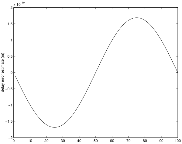
Figure 6: Delay error due to absolute metrology and ACS errors.

6 Summary, conclusions and future plans

SIM astrophysical science is extracted from a model set of equations that relate the measured optical pathlength delay to the projection of the interferometer baseline vector onto the star direction vector. These equations presuppose that the interferometer baseline is fixed in inertial space; which it is not. The main objective of this paper has been to introduce the reader to the concepts and the instrumental logic of the SIM astrometric observations, especially as they relate to the fundamental operation of baseline regularization that “fixes” the interferometer in inertial space. Mathematical arguments were presented to establish this fundamental principle and a precise definition of regularization was given. The underlying nonlinear system of equations that is the basis for regularization was derived and numerical methods to solve them were obtained. A simulation was also developed incorporating the numerical processing methods of the instrument observables and the results were shown to conform with the theory.

Beyond demonstrating the SIM proof of principle, the regularization equations presented here also form the kernel of the extensive instrument error budget. The linearized version of these equations are used to determine the propagation of noise from external metrology measurements and guide star delay measurements to the science delay error. This error is determined by the geometry of the optical truss together with its orientation in inertial space with respect to the guide star and target star positions. The propagation factors are used to set requirements on the integration time of observations, single gauge metrology error, etc. The regularization equations also reveal the existence of a number of second order errors that arise in the form of products of fiducial motion (elastic and rigid body) and initial parameter error. Examples of errors of this type were given.

Current work focuses on the mechanisms and effects of variation of the “constant” terms in the astrometric delay equations. Nominally the appearance of the constant term compensates for the lack of a precise internal metrology gauge that measures the absolute distance between the interferometer aperture fiducials to the beam combiner. However, there are a number of instrument errors that are collected into this single term. For example as the interferometer observes stars within its field of regard several optical elements must be translated and rotated. These induce non–trivial diffraction effects, metrology gauge error due to imperfect corner cubes, reflection phase errors because of a changing angle of incidence of the interrogating metrology beams, and others. Each of these effects must be played through the delay regularization equations to ascertain their ultimate effect on delay error.

References

- [1] R. Danner and S. Unwin, eds., SIM Interferometry Mission: Taking the Measure of the Universe, NASA document JPL 400-811 (1999). Also see http://sim.jpl.nasa.gov/
- [2] A. F. Boden, SIM Astrometric Grid Simulation Development and Performance Assessment, JPL Interoffice Memorandum, 1997.
- [3] R. Swartz, “The SIM Astrometric Grid”, Interferometry in Space, 4852, Proceedings of SPIE, August 2002.
- [4] S. Loiseau, F. Malbet, “Global astrometry with OSI,” A&A Sup., 116, pp.373-380, 1996.
- [5] J. Marr-IV, et al. “Space Interferometry Mission (SIM): Overview and Current Status,” Interferometry in Space, 4852, Proceedings of SPIE, August 2002.
- [6] D. Brady, K.M. Aaron, B.D. Stumm, “Structural design challenges for a shuttle-launched space interferometry mission,” Interferometry in Space, 4852, Proceedings of SPIE, August 2002.
- [7] D.M. Stubbs, R.M. Bell, Jr., S.D. Barrett, T. Kvamme, “Space Interferometry Mission starlight and metrology Subsystems,” Interferometry in Space, 4852, Proceedings of SPIE, August 2002.
- [8] C.E. Bell, “Interferometer real time control development for SIM”, Interferometry in Space, 4852, Proceedings of SPIE, August 2002.
- [9] R.A. Laskin, “SIM technology development overview,” Interferometry in Space, 4852, Proceedings of SPIE, August 2002.
- [10] M. Milman and S. Basinger, “Error sources and algorithms for white-light fringe estimation at low light levels,” Applied Optics, Vol. 41, No. 14, May, 2002, pp. 2655-2671.
- [11] M. Milman, “Optimization approach to the suppression of vibration errors in phase-shifting interferometry”, JOSA A, Vol. 19, No. 5, May, 2002, pp. 992-10004.
- [12] M. Milman, J. Catanzarite, and S. Turyshev, “Effect of wavenumber error on the computation of path-length delay in white-light interferometry,” Applied Optics, Vol. 41, No. 23, August, 2002, pp. 4884-4890.
- [13] F. Zhao, R. Diaz, G. M. Kuan, N. Sigrist, Y. Beregovski, L. L. Ames, K. Dutta, “Internal metrology beam launcher development for the Space Interferometry Mission,” Interferometry in Space, 4852, Proc. of SPIE, August, 2002.
- [14] T. J. Shen, M. Milman, G. Neat, J. Catanzarite, “Dependence of the micro-arcsecond (MAM) testbed performance prediction on white light algorithm approach,” Interferometry in Space, 4852, Proc. of SPIE, August, 2002.
- [15] Slava G. Turyshev, Analytical Modeling of the White Light Fringe. Applied Optics, 42(1), pp.71-90, 2003.
- [16] D.L. Meier, W.M. Folkner, “SIMsim: an end-to-end simulation of SIM”, Interferometry in Space, 4852, Proceedings of SPIE, August 2002.