A model of population dynamics -
further investigations

Abstract

We present supplementary investigations referring to the model of an evolving population described in Physica A 252 (1998) 325–335.

The population is composed of individuals characterised by their genetic strings, phenotypes and ages. We discuss the influence of probabilities of survival of the individuals on the dynamics and phenotypic variability of the population.

We show that constant survival probabilities of individuals are propitious for preserving phenotypic variability of the population. For constant survival probabilities oscillations of ’the average fitness’ of the population and normal distributions of the phenotypes are observed. When the probabilities of survival are directly proportinal to the individuals’ adaptations the population can reach the maximum possible average adaptation, but the phenotypic variability of the population is completely lost and oscillations of ’the average fitness’ of the population do not occur.

We also investigate the behaviour of the population caused by the probabilities of survival that partly depend on the individuals’ adaptations. The role of the length of the individuals’ genetic strings is considered here.

PACS: 87.23; 05.10.L
Keywords: Biological evolution, Population dynamics, Monte Carlo simulations.

1 Introduction

Variability observed in biological populations allows the populations to evolve in different habitats that may in some cases lead to speciation. Natural populations that have low variability are not resistant to changes of their enviromnent and can easily extinct. Preservation of variability is then crucial for biological evolution. Because of this, it has been investigated intensively by biologists (e.g.[1]–[3]), and, in recent years, by physicists (e.g.[4]–[5]). Variability is considered at different levels: phenotypic (the most general), genetic or environmental. Population dynamics is often analysed.

In biological considerations it is usually assumed that at the phenotypic level the distribution of intensity of phenotypic features is normal [6]. In 1996 Doebeli avoided this assumption and presented an interesting model of population dynamics [7]. Some of his intriguing conclusions (described below) were tested in 1998 by Pȩkalski [8], who used a simplified version of the model presented in [9]. In this paper we discuss and develop some of Pȩkalski’s results.

According to Doebeli’s model, a population consists of haploid individuals. Each individual is characterised by a genetic string that has $c$ genes situated at $c$ loci (a locus is the place at a chromosome where a gene is located). Each gene can be in two states: 1 and 0 corresponding to two alleles. Phenotypes of individuals are characterised by ’a character’ $h$ that corresponds to a number of 1’s in its genetic string. The population is infinite. It can be either sexual or asexual. Generations do not overlap.

In case of a sexual population two individuals can create offsprings. The character of an offspring is established by choosing, independently for each locus, an allele from the alleles of the parents with equal probability. The mean fitness of the population, defined as $N(t+1)/N(t)$ (where N(t) denotes the total density of the population at time $t$) and the distribution of the phenotypes existing in the population are controlled. As a result, it is shown that the mean fitness can oscillate and the type of the oscillations depends on the number of loci $c$ . For some parameters, when the total population density is constant, the phenotypes alternate between two distributions. Then, the phenotypic variability of the population is preserved and shows unexpected and very interesting behaviour.

Oscillations of the mean fitness of an evolving polulation and strange distribution of phenotypes inspired Pȩkalski, who tried to confirm Doebeli’s results. He used a lattice model based on the standard Monte Carlo simulations. According to the model, a population is located on a $L\times L$ square lattice. Each lattice site may be either empty or contain an individual. The total initial number of individuals is $N(t=0)$. An individual is characterised by: its location on the lattice $j$, its age $w_{j}$ and its genome. The individual’s age $w_{j}$ is less or equal to the maximum age $M$. $M$ defines the maximum number of Monte Carlo steps (MCS) during which an individual can be a member of the population. If the individual’s age exceedes $M$, the individual is removed from the lattice. The same $M$ is assumed for all individuals. As a parameter, $M$ can vary from 1 to the total duration (in MCS) of a performed simulation. The individual’s genome is assumed to be a string containing $c$ loci with $c$ genes that code $c$ phenotypic features. Genomes and phenotypes are constructed analogically to [7]. During the simulation an individual is chosen randomly, its adaptation is calculated according to the formula:

$$a_{j}={1\over c}\sum_{k=1}^{c}f_{j}^{k}$$ (1)

where $f_{j}^{k}$ denotes the fraction of 1’s in its genetic string. The individual survives if its adaptation is greater than a generated, random number $r\in[0,1]$ (its probability of survival is then strongly connected to the individual’s adaptation). Then the individual moves across the lattice and meets another individual. Movement across the lattice and meeting the neighbour is necessary for mating. Adaptation and probability of survival of the neighbour are calculated. If the neighbour survives, the individuals mate and create offsprings. The offsprings are located on empty sites inside a square $L_{G}\times L_{G}$ centered at the first parent location. The number of the offsprings depends on the number of empty sites of the square. Their maximum number is $q$. The offsprings’ phenotypes are established in the same way as described for Doebeli’s model. After each Monte Carlo step of the simulation the age of all individuals is increased by 1 and all individuals which age exceedes the maximum age $M$ are removed from the population. Since individuals of different age can mate, generations overlap.

In his paper Pȩkalski controlled the time dependence of the density of the population and its average age (relative to the maximum one). In particular he investigated the average adaptation of the population defined by:

$$a(t)={1\over N(t)}\sum_{j=1}^{N(t)}a_{j}(t)$$ (2)

and the ratio of the numbers of individuals in two succeeding moments of time (Monte Carlo steps). He called this quantity the average fitness:

$$<f(t)>={N(t+1)\over N(t)}$$ (3)

As the main result Pȩkalski confirmed Doebeli’s conclusion that oscillatory character of the quantity $N(t+1)/N(t)$ depends on the number of loci of individuals’ genetic strings. The oscillations are damped, their amplitude depends on $c$ and $M$. The period of oscillations depends on $M$. However, in contrast to Doebeli’s results, periodic changes of the distribution of the phenotypes are not observed. It is always normal. Normal distribution of the phenotypes indicates that the population contains individuals better and less adapted. The population does not reach the maximum possible adaptation, but its phenotypic variability is preserved. The maximum possible adaptation would correspond to the situation when the adaptation of every individual equals 1. It is suggested that the population could achieve perfect adaptation, but, as it is shown in Fig.1 of [8] the adaptation of the population seems to stabilise at about 0.7. This conclusion is in contrast to the results described in [10] and [9] where initially random populations quickly reach the maximum possible adaptation $a=1$ (see e.g. [9], Fig.2., first region). This fact should be considered since, as it has been mentioned above, Pȩkalski’s model is a simplified version of the model presented in [9], which bases on the model presented in [10]. The differences between the models are that in [9] a population evolves in two different, spatially separated habitats and individuals are diploids while in [8] a population evolves in one habitat and individuals are haploids. Then it will be interesting to indicate a reason of such big differences among the adaptations of the populations.

2 Simulations and Results

To investigate the conditions under which the adaptation of the population can reach the maximum value and other lower values we have performed computer simulations based on the model described in [8]. We have used the same parameters as in [8]: a $100\times 100$ square lattice, $L_{G}=5$, $q=4$ and $x(0)=0.3$. Averaging has been done over 25 independent runs. The simulations have been performed for the maximum ages $M=5$ and $M=3$ and for the numbers of loci $c=10$, $c=20$ and $c=40$.

We have tested populations in which:

1. Individuals are eliminated from the population only because of aging (when their age is greater than the assumed maximum age). In this case probability of survival is $p=1.00$.

2. Individuals are eliminated with some constant probability $1-p$, where survival probability $p$=0.95; 0.90; 0.85; 0.80. Moreover they are eliminated because of their age.

3. Probability of survival depends on individuals’ adaptation, calculated according to the formula (1), as assumed in [8]. They are also eliminated because of their age.

When the population evolves with the probability of survival $p=1.00$, large oscillations of $N(t+1)/N(t)$ are observed. The period of the oscillations depends on $M$ (Fig.1), but none of the features of the oscillations depends on $c$.

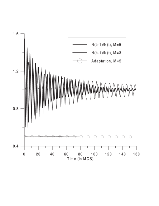
Figure 1: Time dependence of $N(t+1)/N(t)$ and the average adaptation of the population for different maximum ages $M$. Probability of survival of individuals $p=1.00$. Number of loci $c=20$.

This can be explained as follows: before creating offsprings an individual has to move and meet a neighbour. When the population density is high, the individual can not move. Even if it manages to move and meets the neighbour, there is not enough space for many offsprings. Individuals have to be eliminated because of aging, then the population density becomes lower, some space required for mating occurs and new offsprings are created. At the beginning of the simulations phenotypes are randomly chosen so the average adaptation of the population is 0.5. Since there are not many factors that may influence the average adaptation (individuals are eliminated only because of their age), the population is never adapted well and its average adaptation is constant (equals 0.5).

When individuals are eliminated with some constant probability, independently on their adaptation, the average adaptation of the population is also low and constant (still equals 0.5). The oscillations of $N(t+1)/N(t)$ are however smaller (Fig.2). The additional mechanism of individuals’ elimitation causes that there is more free space on the lattice. This results in perturbations of big, age-dependent oscillations.

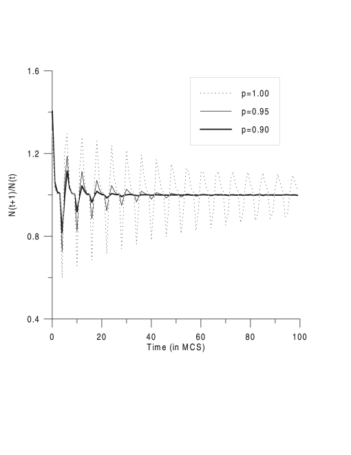
Figure 2: Time dependence of $N(t+1)/N(t)$ for different probabilities of survival of individuals. Number of loci $c=20$. Maximum age $M=5$.

When probability of survival depends on the individual’s adaptation, the population achieves the maximum possible adaptation and, in contrast to the results presented in [8], it reaches the average adaptation equal 1 independently on the number of loci $c$ (Fig.3). Oscillations of $N(t+1)/N(t)$ are not observed here (Fig.4). When the average adaptation of the population equals 1 all individuals are identical - their genetic strings contain only 1’s. Then, a typical, normal distribution of phenotypes is not observed and the phenotypic variability of the population is lost.

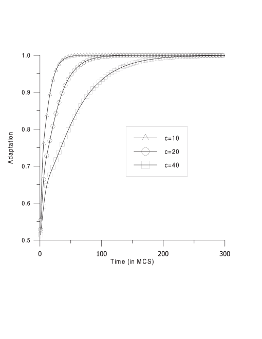
Figure 3: Time dependence of the average adaptation of the population when the probability of survival of an individual strongly depends on its adaptation. Maximum age $M=5$. The parameter is the number of loci $c$.

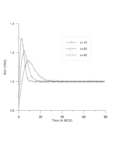
Figure 4: Time dependence of $N(t+1)/N(t)$ when the probability of survival of an individual strongly depends on its adaptation. Maximum age $M=5$. The parameter is the number of loci $c$.

The above described procedures lead to two types of populations: a badly adapted one and a perfectly adapted one. The average adaptation of 0.7 presented in [8] seems to be an intermediate case.

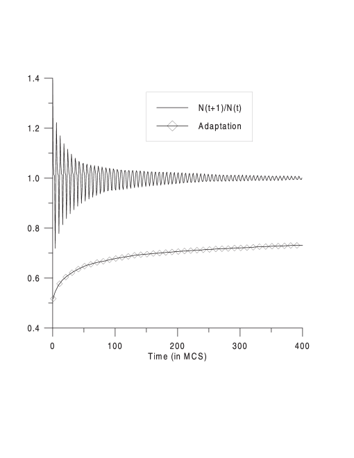
Figure 5: Time dependence of $N(t+1)/N(t)$ and the average adaptation of the population. Probability of survival of an individual depends on its adaptation according to (4). Number of loci $c=20$, $B=10$. Maximum age $M=5$.

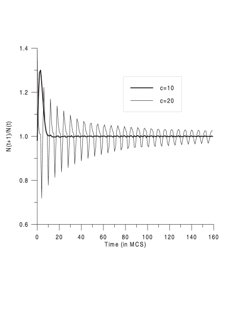
Figure 6: Time dependence of $N(t+1)/N(t)$. Probability of survival of an individual depends on its adaptation according to (4). $B=10$. Maximum age $M=5$. The parameter is the number of loci $c$.

It is possible to obtain such an average adaptation if the probability of survival of an individual depends on its adaptation, but not so strongly as the probability calculated previously, according to the formula (1). For example, (1) can be transformed to

$$A_{j}={1\over B}\sum_{k=1}^{c}f_{j}^{k}$$ (4)

where $B$ is a constant equal or smaller than $c$. $A_{j}$ may be considered as an individual’s adaptation, but it must be assumed that all values of $A_{j}$ equal or greater than 1 denote perfect adaptation. For example, let $c=20$ and $B=10$. The individuals that have ten or more 1’s in their phenotypes will surely survive ($A_{j}=1$ for ten 1’s and $A_{j}$ is greater than 1 for more than ten 1’s. The maximum possible $A_{j}=2$ characterises an individual with all 1’s in its phenotype). Therefore, only really badly adapted individuals can be eliminated. The effect becomes stronger for increasing $c$. At the same time, perfectly adapted individuals, eliminated only because of their age, may cause oscillations of $N(t+1)/N(t)$.

Now it is possible to receive oscillating $N(t+1)/N(t)$ and the average adaptation of a population that is between 0.5 and 1. The results for $c=20$ and $B=10$ are presented in Fig.5.

When $B=10$ and $c=10$ the formulas (1) and (4) are identical. Fig.6 presents the time dependence of $N(t+1)/N(t)$ for different $c$. Probability of survival is calculated using the formula (4). There is some similarity between the results presented in Fig.5 and Fig.6 and, respectively, Fig.1 and Fig.2 of [8].

3 Conclusions

To summarise, for the presented model the oscillatory character of $N(t+1)/N(t)$ and values of the average adaptation of the population depend on the way how individuals are eliminated from the population.

1. When the individuals are eliminated only because of exceeding the maximum possible age, big, damped oscillations of $N(t+1)/N(t)$ are observed while the average adaptation is low. In this case high phenotypic variability (and normal distribution of phenotypes) is preserved.

2. The oscillations can be reduced without affecting the phenotypic variability of the population if the individuals are eliminated with some constant probability.

3. If the individual’s survival probability depends on the individual’s adaptation and it is calculated according to the formula (1), the oscillations of $N(t+1)/N(t)$ do not occur and the population quickly reaches perfect adaptation. All individuals are identical and the population has no phenotypic variability.

4. When individuals characterised by the lowest adaptation are eliminated according to the formula (4) it is possible to observe many values of the average adaptation of the population and oscillations of $N(t+1)/N(t)$. In this case the population can be better adapted than when the indivduals are eliminated because of aging. Moreover, the phenotypic variability of the population is preserved. The average adaptation of the population depends on the number of individuals’ phenotypic features (the number of phenotypic features of an individual equals the number of loci $c$ in its genetic string). Then, populations composed of organisms that have different $c$ might evolve in a different way: for small $c$ the phenotypic variability would be lost while for bigger $c$ the phenotypic variability would be preserved. Therefore, for populations characterised by small $c$ other mechanisms, for example mutations, should be introduced to keep the variability. This case seems to be interesting also from biological point of view and we hope that we will investigate it in details.

Acknowledgements
This work was supported by The State Committee for Scientific Research (grant no. 2PO3B 149 18) and University of Wrocław (grant no. 2016/ W/ IFD/ 02).
I also thank Professor Andrzej Pȩkalski (Institute of Theoretical Physics, University of Wrocław) for discussion and Professor Marcel Ausloos (University of Liège) for his valuable comments.

References

- [1] N.H. Barton, Genet. Res. 47 (1986) 209.
- [2] T. Kawecki, Proc. R. Soc. Lond. B, 263 (1996) 1515.
- [3] M. Doebeli, G.D. Ruxton, Evolution, 51 (1997) 1730.
- [4] P. Derrida, P. Higgs, J. Phys. A 24 (1991) L985.
- [5] L. da Silva, C. Tsallis, Physica A, 271 (1999) 470.
- [6] M. Slatkin, Ecology, 61 (1980) 163.
- [7] M. Doebeli, Evolution, 50 (1996) 532.
- [8] A. Pȩkalski, Physica A, 252 (1998) 325.
- [9] I. Mróz, A. Pȩkalski, Eur. Phys. J. B 10 (1999) 181.
- [10] I. Mróz, A. Pȩkalski, K. Sznajd–Weron, Phys Rev. Lett. 76 (1996) 3025.