What causes a neuron to spike?

Abstract

The computation performed by a neuron can be formulated as a combination of dimensional reduction in stimulus space and the nonlinearity inherent in a spiking output. White noise stimulus and reverse correlation (the spike-triggered average and spike-triggered covariance) are often used in experimental neuroscience to ‘ask’ neurons which dimensions in stimulus space they are sensitive to, and to characterize the nonlinearity of the response. In this paper, we apply reverse correlation to the simplest model neuron with temporal dynamics—the leaky integrate-and-fire model—and find that even for this simple case standard techniques do not recover the known neural computation. To overcome this, we develop novel reverse correlation techniques by selectively analyzing only ‘isolated’ spikes, and taking explicit account of the extended silences that precede these isolated spikes. We discuss the implications of our methods to the characterization of neural adaptation. Although these methods are developed in the context of the leaky integrate-and-fire model, our findings are relevant for the analysis of spike trains from real neurons.

1 Introduction

There are two distinct approaches to characterizing a neuron based on spike trains recorded during stimulus presentation. One can take the view of a downstream neuron, and ask how the spike train should be decoded to reconstruct some aspect of the stimulus. Alternatively, one can take the neuron’s own view, and try to determine how the stimulus is encoded, i.e. which aspects of the stimulus trigger spikes. This paper is concerned with the latter problem: the identification of relevant stimulus features from neural data.

The earliest attempts at neural characterization, including classic electrophysiological experiments like those of Adrian [1], presented the neural system with simple, highly stereotyped stimuli with one or at most a few free parameters; this makes it relatively straightforward to map the input/output relation, or tuning curve, in terms of these parameters. While this approach has been invaluable, and is still often used to advantage, it has the shortcoming of requiring a strong assumption about what the neuron is ‘looking for’. As this assumption is relaxed by probing the system using stimuli with a larger number of parameters, the length of the experiment needed to probe neural response grows combinatorially.

In some cases, white noise can be used as an alternative stimulus which naturally contains ‘every’ signal [2]. The stimulus feature best correlated with spiking is then the spike triggered average (STA), i.e. the average stimulus history preceding a spike [3, 4]. Such reverse correlation methods have been further developed and applied to characterize the motion-sensitive identified neuron H1 in the fly visual system [5]. By extending reverse correlation to second order, one can identify multiple directions in stimulus space relevant to the neuron’s spiking ‘decision’ [6, 7]. These techniques allow the experimenter to probe neural response stochastically, using minimal assumptions about the nature of the relevant stimulus.

In this paper, we will examine in detail the relation between the stimulus features extracted through white noise analysis and the computation actually performed by the neuron. In the usual interpretation of white noise analysis, the features extracted using reverse correlation are considered to be linear filters which, when convolved with the stimulus, provide the relevant inputs to a nonlinear spiking decision function. While the features recovered by reverse correlation are optimal for stimulus reconstruction [8], we will show that they are distinct from the filter or filters relevant to the neuron’s spiking decision. In particular, reconstruction filters necessarily depend on the stimulus ensemble, while the filters relevant for spiking—at least, for simple neurons like leaky integrate-and-fire—are properties of the model alone.

The main difficulty in interpreting the spike triggered average is that spikes interact, in the sense that the occurrence of a spike affects the probability of the future occurrence of a spike. Both stimulus reconstruction and the identification of triggering features are affected by this issue. Some of the effects of correlations between spikes have been treated in [9, 10, 11, 12]. To separate the influence of previous spikes from the influence of the stimulus itself, we propose to analyze only ‘isolated’ spikes—spikes sufficiently distant in time from previous spikes that they can be considered to be statistically independent. This procedure allows us to recover exactly the relevant stimulus features. However, it introduces additional complications. By requiring an extended silence before a spike, we bias the prior statistical ensemble. This bias will emerge in the white noise analysis, and we will have to identify it explicitly.

We carry out this program for the simplest model neuron with temporal dynamics: the leaky integrate-and-fire neuron. We choose this model because, unlike more complex models, we know exactly which stimulus feature causes spiking, and can make a precise comparison with the output of the analysis.

The methods presented and validated in the present work using the integrate-and-fire model have been applied to the more biologically interesting Hodgkin–Huxley neuron [13], resulting in new insights into its computational properties. Application of the same analytic techniques to real neural data is currently underway.

2 Characterizing neural response

In this section we briefly review material that has appeared elsewhere [14, 13, 7].

2.1 The linear/nonlinear model

Consider a neuron responding to a dynamic stimulus $I(t)$. While here we will consider $I$ to be a scalar function, in general, it may depend on any number of additional variables, such as frequency, spatial position, or orientation. We can suppress these dependencies without loss of generality. Even without additional dependent variables, $I(t)$ is a high-dimensional stimulus, as the occurrence of a spike at time $t_{0}$ generally depends on the stimulus history, $I(t<t_{0})$. The effective dimensionality of this input is determined by the temporal extent of the relevant stimulus, and the effective sampling rate, which is imposed by biophysical limits. For the computation of the neuron to be characterizable at all, the dimensionality of the stimulus relevant to spiking must generally be much lower than this total dimensionality. The simplest approach to dimensionality reduction is to approximate the relevant dimensions as a low-dimensional linear subspace of $I(t)$.

If the neuron is sensitive only to a low dimensional linear subspace, we can define a small set of signals $s_{1},s_{2},\cdots,s_{K}$ by filtering the stimulus,

$$s_{\mu}=\int_{0}^{\infty}d\tau f_{\mu}(\tau)I(t_{0}-\tau)\,,$$ (1)

so that the probability of spiking depends only on these few signals,

$$P[{\rm spike\,at\,}t_{0}|I(t<t_{0})]=P[{\rm spike\,at\,}t_{0}]\,g(s_{1},s_{2},\cdots,s_{K})\,.$$ (2)

Classic characterizations of neurons in the retina, for example [15], typically assume that these neurons are sensitive to a single linear dimension of the stimulus; the filter $f_{1}$ then corresponds to the (spatiotemporal) receptive field, and $g$ is proportional to the one-dimensional tuning curve. A number of other neurons, particularly early in sensory pathways, have been similarly characterized, e.g. [16, 17, 18]. Here we will concentrate primarily on the problem of finding the filters $\{f_{\mu}\}$; once they are found, $g$ can be obtained easily by direct sampling of $P[{\rm spike\,at\,t_{0}}|s_{1},s_{2},\cdots,s_{K}]$, assuming that the relevant dimensionality $K$ is small.

2.2 Reverse correlation methods

While one would like to determine the neural response in terms of the probability of spiking given the stimulus, $P[{\rm spike\,at\,}t_{0}|I(t<t_{0})]$, we follow [5] in considering instead the distribution of signals conditional on the response, $P[I(t<t_{0})|{\rm spike\,at\,}t_{0}]$. This quantity can be extracted directly from the known stimulus and the resulting spike train. The two probabilities are related by Bayes’ rule,

$${{P[{\mathrm{spike}\,\mathrm{at}\,}t_{0}|I(t<t_{0})]}\over{P[{\mathrm{spike}\,\mathrm{at}\,}t_{0}]}}={{P[I(t<t_{0})|{\mathrm{spike}\,\mathrm{at}\,}t_{0}]}\over{P[I(t<t_{0})]}}\,.$$ (3)

$P[\mathrm{spike}\,\mathrm{at}\,t_{0}]$ is the mean spike rate, and $P[I(t<t_{0})]$ is the prior distribution of stimuli. If $I(t)$ is Gaussian white noise, then this distribution is a multidimensional Gaussian; furthermore, the distribution of any filtered version of $I(t)$ will also be Gaussian.

The first moment of $P[I(t<t_{0})|{\rm spike\,at\,}t_{0}]$ is the spike-triggered average,

$$\mathrm{STA}(\tau)=\int[dI]\,P[I(t<t_{0})|{\rm spike\,at\,}t_{0}]I(t_{0}-\tau)\,.$$ (4)

We can also compute the covariance matrix of fluctuations around this average,

$$C_{\rm spike}(\tau,\tau^{\prime})=\int[dI]\,P[I(t<t_{0})|{\rm spike\,at\,}t_{0}]I(t_{0}-\tau)I(t_{0}-\tau^{\prime})-\mathrm{STA}(\tau)\mathrm{STA}(\tau^{\prime}).$$ (5)

In the same way that we compare the spike-triggered average to some constant average level of the signal in the whole experiment, an important advance of [6] was to compare the covariance matrix $C_{\rm spike}$ with the covariance of the signal averaged over the whole experiment,

$$C_{\rm prior}(\tau,\tau^{\prime})=\int[ds]\,P[s(t<t_{0})]s(t_{0}-\tau)s(t_{0}-\tau^{\prime})\,.$$ (6)

If the probability of spiking depends on only a few relevant features, the change in the covariance matrix, $\Delta C=C_{\rm spike}-C_{\rm prior}$, has a correspondingly small number of outstanding eigenvalues. Precisely, if $P[{\rm spike}|{\rm stimulus}]$ depends on $K$ linear projections of the stimulus as in Eq. (2), and if the inputs $I(t)$ are chosen from a Gaussian distribution, then the rank of the matrix $\Delta C$ is exactly $K$. Further, the eigenmodes associated with nonzero eigenvalues span the relevant subspace. A positive eigenvalue indicates a direction in stimulus space along which the variance is increased relative to the prior, while a negative eigenvalue corresponds to reduced variance.

3 Leaky integrate-and-fire

The leaky integrate-and-fire neuron is perhaps the most commonly used approximation to real neurons. Its dynamics can be written:

$$C{{dV}\over{dt}}=I(t)-{V\over R}-CV_{c}\sum_{i}\delta(t-t_{i})\,,$$ (7)

where $C$ is a capacitance, $R$ is a resistance and $V_{c}$ is the voltage threshold for spiking. The first two terms on the right hand side model an RC circuit; the capacitor integrates the input current as a potential $V$ while the resistor dissipates the stored charge (hence ‘leaky’). The third term implements spiking: spikes are defined as the set of times $\{t_{i}\}$ such that $V(t_{i})=V_{c}$. When the potential reaches $V_{c}$, a restoring current is instantaneously injected to bring the stored charge back to zero, resetting the system. This formulation emphasizes the similarity between leaky integrate-and-fire and the more biophysically realistic Hodgkin–Huxley equation for current flow through a patch of neural membrane; in the Hodgkin–Huxley system, however, the nonlinear spike-generating term is replaced with ionic currents of a more complex (and less singular) form. Hence the simple properties of the leaky integrate-and-fire model—a single degree of freedom $V$, instantaneous spiking, total resetting of the system following a spike, and linearity of the equation of motion away from spikes—are only rough approximations to the properties of realistic neurons.

Integrating Eq. (7) away from spikes, we obtain

$$CV(t)=\int_{-\infty}^{t}d\tau\exp\left({\tau-t}\over{RC}\right)I(\tau)\,,$$ (8)

assuming initialization of the system in the distant past at zero potential. The right hand side can be rewritten as the convolution of $I(t)$ with the causal exponential kernel

$$f_{\infty}(\tau)=\left\{\begin{array}[]{ll}0&\mbox{if $\tau\leq 0$}\\ \exp(-\tau/RC)&\mbox{if $0<\tau$,}\end{array}\right.$$ (9)

so the condition for a spike at time $t_{1}$ is that this convolution reach threshold:

$$CV_{c}=\int_{-\infty}^{\infty}d\tau f_{\infty}(\tau)I(t_{1}-\tau)\,.$$ (10)

The interaction between spikes complicates this picture somewhat. If the system spiked last at time $t_{0}<t_{1}$, we must replace the lower limit of integration in Eq. (8) with $t_{0}$, as no current injected before $t_{0}$ can contribute to the accumulated potential. However, if we wish always to evaluate stimulus projections by integrating over the entire current history $I(t)$ as in Eq. (10), then we must replace $f_{\infty}$ with an entire family of kernels dependent on the time to the previous spike, $\Delta t=t_{1}-t_{0}$:

$$f_{\Delta t}(\tau)=\left\{\begin{array}[]{lll}0&\mbox{if $\tau\leq 0$}\\ \exp(-\tau/RC)&\mbox{if $0<\tau<\Delta t$}\\ 0&\mbox{if $\Delta t\leq\tau$.}\end{array}\right.$$ (11)

This equation completes an exact model of the leaky integrate-and-fire neuron.

4 Response to white noise

We now consider the statistical behavior of the integrate-and-fire neuron when driven with Gaussian white noise current of standard deviation $\sigma$,

$$\langle I(t)\rangle = 0,$$

$$\langle I(t)I(t^{\prime})\rangle = \sigma^{2}\delta(t-t^{\prime}).$$ (12)

For the following analysis, we take $R=10$ k$\Omega$, $C=1$ $\mu$F, $V_{c}=10$ mV and $\sigma=\sqrt{200}$ $\mu$A, and use Euler integration with a time step of 0.05 msec. These values were chosen to mimic biophysically plausible parameters for a 1 $\mathrm{cm}^{2}$ patch of membrane, but none of our results depend qualitatively on this choice.

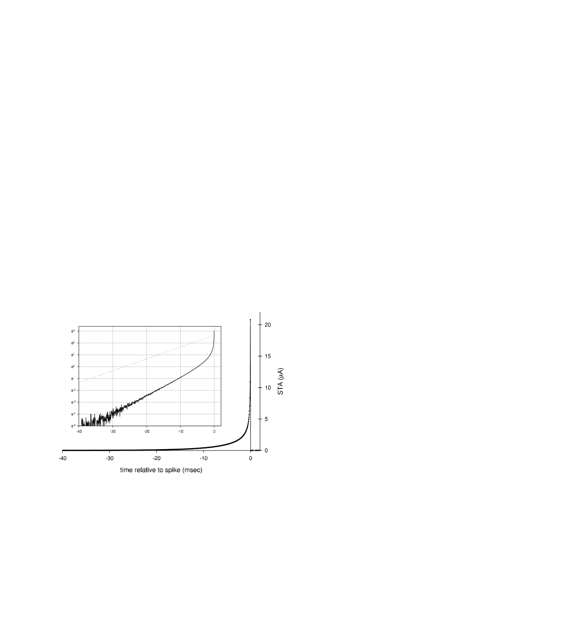
Figure 1: Spike-triggered average of a leaky integrate-and-fire neuron; shown inset with a logarithmic $I$-axis and the pure exponential $\sigma f_{\infty}$ (dotted line).

4.1 Unqualified reverse correlation

At first glance, it would appear that the neuron is perfectly described by a reduced model in one dimension: the current filtered by the exponential kernel of Eq. (9). If so, the spike-triggered average under white noise stimulation should be proportional to this filter. However, as is evident in Fig. 1, the STA is not exponential, nor does it asymptote to the appropriate decay rate $1/RC$. One reason is that, in the presence of previous spikes, the integrate-and-fire neuron is not low-dimensional. Recall that the relative timing $\Delta t$ of the previous spike selects a filter $f_{\Delta t}$ (Eq. (11)); these filters are truncated versions of the original exponential $f_{\infty}$. The STA will therefore include contributions from each of these filters, weighted by their probability of occurrence (as determined by the interspike interval distribution). It is readily shown that the orthogonal component of each filter $f_{\Delta t}$ is a $\delta$-function at $-\Delta t$; so the set of relevant filters spans the entire stimulus space.

Covariance analysis reveals this high dimensionality very clearly. In Fig. 2 we show the spectrum of eigenvalue magnitudes of $\Delta C$ as a function of the number of spikes summed to accumulate the matrix; with decreasing noise, an arbitrary number of significant eigenmodes emerge. As shown in Fig. 3, none of these eigenmodes correspond to an exponential filter. The first mode most closely resembles an exponential, but as shown in the right half of Fig. 3, it is more peaked near $t=0$, and its time constant is very different from $RC$.

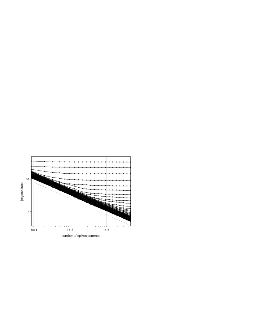
Figure 2: Eigenvalue magnitudes of the spike-triggered covariance difference matrix $\Delta C$ as a function of the number of spikes used to accumulate the matrix. An arbitrary number of stable modes emerge, given enough data. The stable modes all have negative eigenvalues, i.e. spikes are associated with reduced stimulus variance along these dimensions. The dotted line, shown for reference, is proportional to $1/\sqrt{N_{\rm spikes}}$.

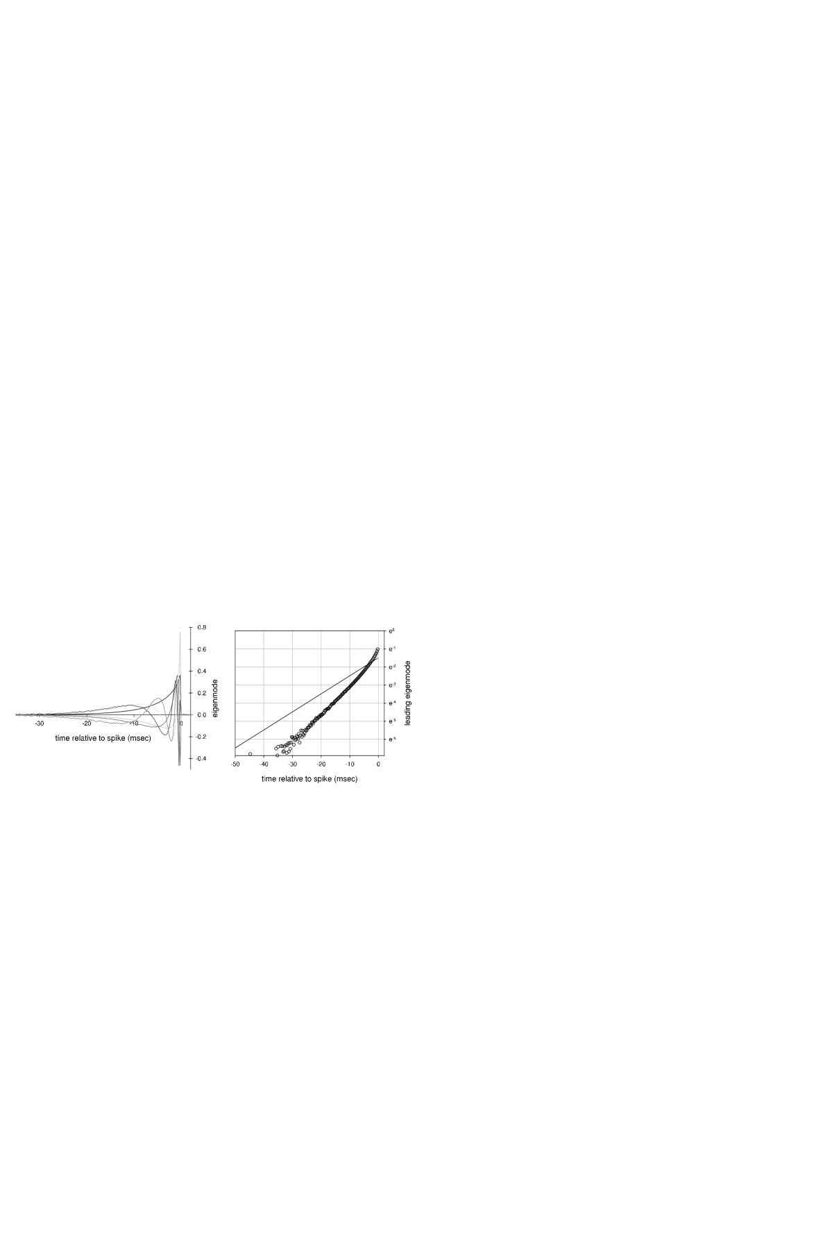
Figure 3: Left: the leading six modes of the unqualified spike-triggered change in covariance $\Delta C$. Right: only the first mode is monophasic; here it is plotted on a logarithmic $y$-axis (circles) with $f_{\infty}$ for reference (solid line).

4.2 Isolated spikes

It is clear that making progress requires first considering the causes of a single spike independently of the spiking history. Therefore we will include in our analysis only spikes which follow previous spikes after a sufficiently long interval. The appropriate interval can be estimated from the interspike interval distribution, Fig. 4.

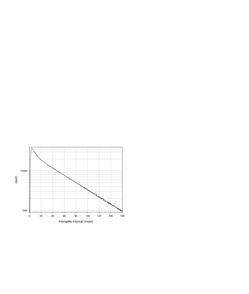
Figure 4: Interspike interval histogram for a leaky integrate-and-fire neuron. $5\times 10^{6}$ spikes were accumulated in $0.27$ msec bins.

As in many real neurons, the interval distribution has three main features: a ‘refractory period’ during which spikes are strongly suppressed, a peak at a preferred interval, and an exponential tail. Intervals in the exponential tail follow Poisson statistics; for intervals in this range, we can take spikes to be statistically independent. With reference to Fig. 4, we set our isolated spike criterion—very conservatively—as 75 msec of previous ‘silence’.

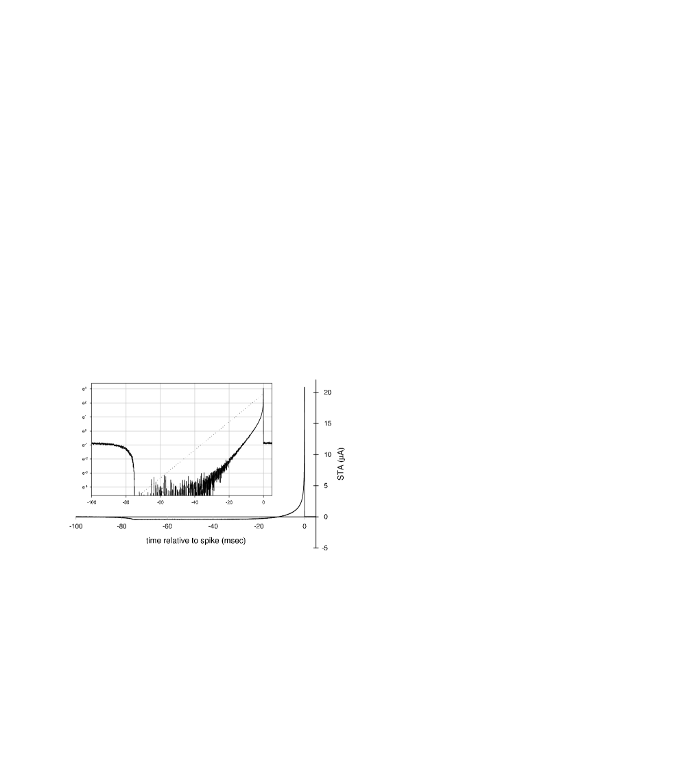
Figure 5: Triggered average stimulus for isolated spikes. Isolated spikes are defined as spikes which are preceded by at least 75 msec of silence. The inset shows the triggered average with the constant silence bias subtracted on a logarithmic $I$-axis, again with the pure exponential $\sigma f_{\infty}$ drawn as a dotted line for reference.

As shown in Fig. 5, even with this constraint, we do not recover a spike-triggered average matching $f_{\infty}$. We should note that this is no longer, strictly speaking, a spike-triggered average, but an event-triggered average, where the event includes the preceding silence. Thus we can expect the silence itself to contribute to any average we construct. To first order, during silence there is a constant negative bias, since certain positive currents which would have caused a spike are excluded from the average. Similarly, we expect that the covariance of the current will be altered from that of the Gaussian prior during extended silences. Because extended silence is not locked to any particular moment in time, the covariance matrix is stationary during silence.

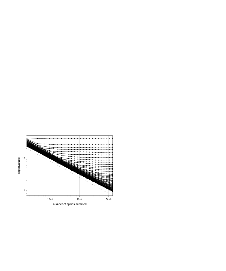
Figure 6: Eigenvalue magnitudes of the isolated spike-triggered change in covariance $\Delta C_{\rm iso}$ as a function of the number of isolated spikes used to accumulate the matrix. The stable modes again have negative eigenvalues.

We construct the covariance matrix as before: $\Delta C_{\rm iso}=C_{\rm isolated\,spike}-C_{\rm prior}$. An entire series of modes once again appears, Fig. 6. This time, they arise because silence is, by definition, translationally invariant, resulting in a Fourier-like spectrum. Modes associated with the spike, on the other hand, are locked to a particular time, and should therefore not have Fourier-like modes. In particular, these spiking modes should have temporal support only in the time immediately before the spike. This implies that two types of modes—silence- and spike-associated—should emerge independently in the covariance analysis, and should exhibit a clear difference in their domain of support.

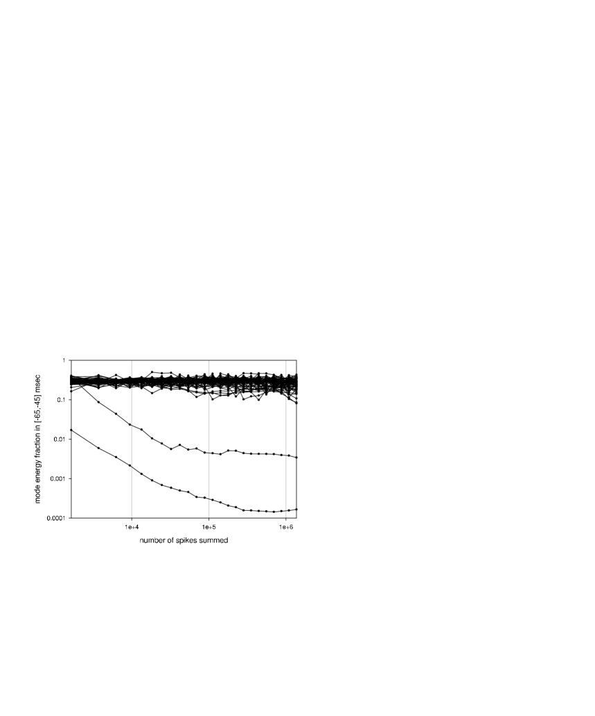
Figure 7: Fraction of the energy in each mode of $\Delta C_{\rm iso}$ (modes are defined over $t\in[-65,0]$ msec) in the silent interval $t\in[-65,-45]$ msec, as a function of the number of isolated spikes used to accumulate $\Delta C_{\rm iso}$. The eigenvalue for a mode with zero energy in this interval would decrease like $1/N_{\rm spikes}$, as the only contribution would come from noise. Here, two modes emerge with very small energy in this interval, though they stabilize at small nonzero values. These modes are localized to the time immediately before the spike, but as they have exponential support, their energy in the silence does not fall all the way to zero.

In Fig. 7, we consider the fraction of the energy of each mode over the interval $t\in[-65,-45]$ msec. At $-45$ msec, the exponential filter $f_{\infty}$ has decayed to 1% of its peak value, so we are well away from the spike at $t=0$. The 75 msec silence criterion also puts the lower boundary of this interval well inside the stationary silence (at least 10 msec after the previous spike). As we see, exactly two modes emerge as local, with their energy fraction decaying with the noise in the matrix until reaching a stable value well below the rest of the modes.

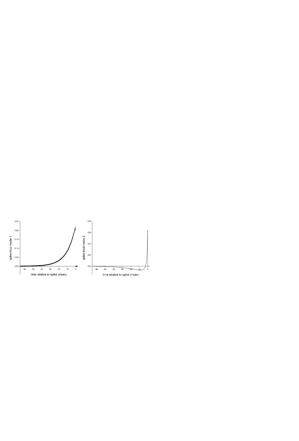
Figure 8: The two spike-associated modes of $\Delta C_{\rm iso}$. The first (left) is the recovered exponential filter of the leaky integrate-and-fire spiking condition; the measured mode is marked with dots, and the line is $f_{\infty}$ (normalized). The second mode (right) is the ‘first crossing’ constraint.

The first localized mode, shown in Fig. 8, is the long-awaited exponential filter $f_{\infty}$. Using our modified second-order reverse correlation analysis on ‘experimental data’ we have thus finally been able to recover the stimulus feature to which the leaky integrate-and-fire neuron is sensitive.

4.3 Constraints

The second mode is a consequence of an implicit constraint in the spiking model. Naïvely, we know that at the moment when $V=V_{c}$, $\dot{V}>0$; that is, the threshold must be crossed from below. Hence

$$\int_{-\infty}^{\infty}d\tau I(t-\tau){d\over{d\tau}}f_{\infty}(\tau)<0,$$ (13)

making the neuron also sensitive to the time derivative of $f_{\infty}$. The integrate-and-fire neuron is peculiar in that $f_{\infty}$ and $df_{\infty}/d\tau$ are almost linearly dependent:

$${d\over{d\tau}}f_{\infty}(\tau)=\left\{\begin{array}[]{ll}\delta(\tau)&\mbox{if $\tau\leq 0$.}\\ -(RC)^{-1}\exp(-\tau/RC)&\mbox{if $0<\tau$.}\end{array}\right.$$ (14)

The orthogonal part of this filter is therefore only $\delta(\tau)$, and we can rewrite this extra condition more simply as $I(0)>V_{c}/R$.

However, we see that although the second spiking mode is indeed very sharply peaked at $\tau=0$, it is not a $\delta$-function. While the above argument is correct in constraining the possible values of $I(0)$, we have also required no threshold crossings for an extended time prior to the spike. Hence certain trajectories $I(t)$ which satisfy the two basic conditions ($V(0)=V_{c}$ and $\dot{V}(0)>0$) are still disallowed, because they would have led to a spike earlier. The second mode is therefore an extended version of the derivative condition. Although it appears to have very extended support, this is due to orthogonalization with respect to the first mode, $f_{\infty}$. The true constraint is positive definite and highly peaked, with virtually all of its energy concentrated in the $\sim 5$ msec interval prior to the spike.

We can more easily understand this constraint by considering the time-dependent distribution of $V(t)$ leading up to an isolated spike, shown in the left panel of Fig. 9. The process $V(t)$ leading up to a spike is a centrally biased random walk with an absorbing barrier at $V_{c}$ and a capacitatively determined correlation time. If we trace the distribution of $V$ backward in time from the spike at $t=0$, we see a constrained diffusive process from a $\delta$-function at the spike time to the steady-state silence distribution. The constraint on $V$ enforces a corresponding constraint on $I$, whose time-dependent distribution is shown in the right panel of Fig. 9. Notice that the $I$ distribution is only noticeably distorted from its silence steady-state at times very near the spike.

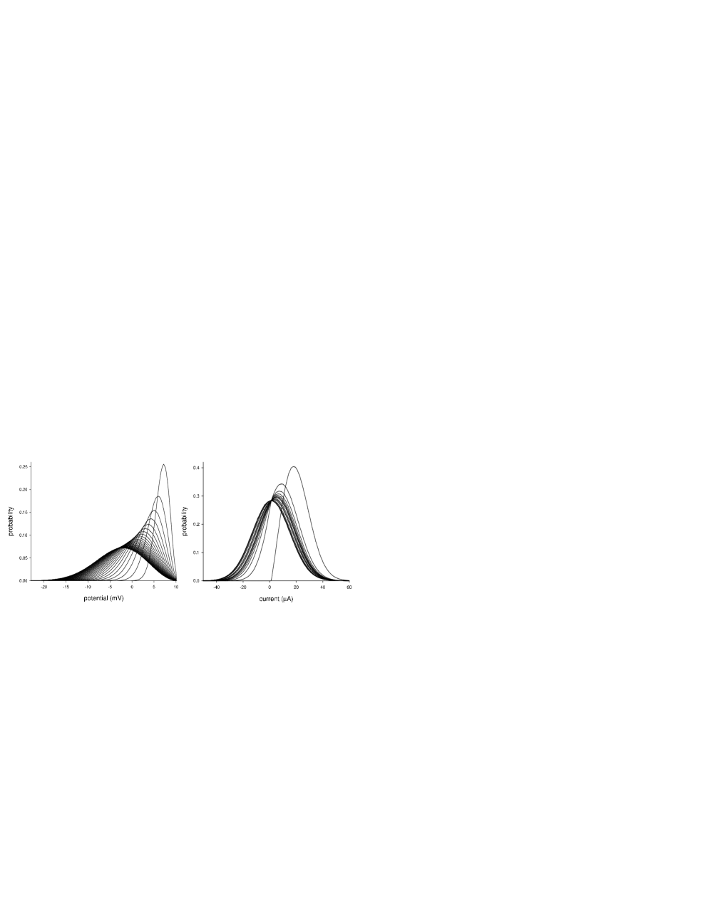
Figure 9: The time-dependent distributions of $V(t)$ (left) and $I(t)$ (right) leading up to an isolated spike at $t=0$. In both cases, the distributions with the highest means correspond to the final time slice (they are thus also the most constrained). For $V$, the times shown are $\{-15,-14.5,-14,\,\cdots\,,-1.5,-1,-0.5\}$ msec. For $I$, the times are $\{-5.05,-4.05,\,\cdots\,,-1.05\}$, $\{-0.8,-0.6,-0.4\}$, and $\{-0.35,-0.3,\,\cdots\,,-0.05\}$ msec. The distribution of $V$ is virtually indistinguishable from its silence steady-state by $-15$ msec; convergence to the silence steady-state is much faster for $I$, occurring by $-5$ msec.

4.4 Silence modes

Finally, let us return to the spectrum of silence-associated modes in Fig. 7. Several of these are shown overlaid in Fig. 10. It is immediately clear that they have the expected Fourier-like structure over the period of silence. Their behavior near the spike is less obvious, however: each mode appears to execute an FM chirp, culminating in a sharp feature at the spike time itself. Clearly, while it is true by construction that spike-associated covariance modes have no support in periods of extended silence, the converse is not true. This structure is due to the essential non-stationarity of silence near spikes: at some point, the silence must come to an abrupt end.

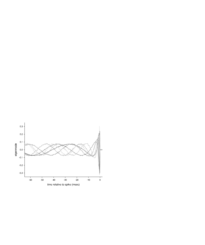
Figure 10: The leading six modes of $\Delta C_{\rm iso}$ associated with silence (i.e. with nonvanishing support over $t\in[-65,-45]$ msec). Although they are Fourier-like in the silence, they chirp leading up to the spike.

It is clear that in order to implement our procedure for separating silence from spikes, we could not have taken the approach of looking for modes with significant energy near the spike. All of the silence modes have interesting structure near the spike, and could easily be mistaken for additional spike-generating features. Like the spike-associated modes, these silence modes have negative eigenvalues, indicating reduced stimulus variance in certain dimensions. Yet they do not cause spiking, nor do they inhibit it; they are in no meaningful sense ‘suppressive’ modes. They simply show us the second-order statistics of silences, which emerge from the enforced absence of spikes. This underscores the necessity of considering a sufficiently extended silence before isolated spikes for the translationally invariant part of the silence modes to emerge, distinguishing them from spiking modes.

This structure also highlights the reason why we could not, as one might expect, simply subtract from $C_{\rm isolated\,spike}$ a prior obtained from extended silences instead of $C_{\rm prior}$ to obtain a simple, low-dimensional $\Delta C_{\rm iso}$. While such a subtraction results in a local matrix around the spike, it cannot take into account the non-stationary part of the silence, and leaves the spike-related and non-stationary silence-related aspects of the covariance near the spike mixed. This again results in a high-dimensional matrix with incorrect (mixed) modes.

5 Adaptation

It has previously been observed that the STAs of some neurons depend on the stimuli used to probe their response [16, 19]. White noise stimulus was originally introduced to circumvent this difficulty by sampling stimulus space in an unbiased way; however, one must still choose a noise variance. While one would hope that this does not affect the STA, it has been shown that, at least in some sense, even the integrate-and-fire neuron ‘adapts’ to the stimulus variance [20, 18], showing both a change in the overall STA and in its measured nonlinear decision function. The reason for this form of adaptation is simple: the statistics of spike intervals depend on the stimulus variance, as the time to reach threshold depends on the variance. By construction, however, neither the spike-triggering feature $f_{\infty}$ nor the decision function $g$ (here simply the threshold) of the integrate-and-fire neuron actually depends on the stimulus statistics. As we have discussed, the unqualified STA is a linear combination of the filters $f_{\Delta t}$ conditioned on the time to the last spike; the contribution of each filter to the overall STA thus depends on the probability $P(\Delta t)$ of the interspike interval $\Delta t$. As different stimulus ensembles produce different interspike interval distributions, these coefficients are functions of the stimulus ensemble. Therefore even in the absence of adaptation in the linear filters $f$, the overall STA will be stimulus-dependent. Because sampling the input/output relation normally involves convolving the stimulus with the STA, the measured nonlinearity will also appear to be stimulus-dependent, despite the fact that the neuron’s nonlinear decision function $g$ (based on convolution of the stimulus with the fixed filters $f$) is also fixed. Hence this form of ‘adaptation’ does not reflect any changing property or internal state of the neuron in response to the stimulus statistics. Rather, it arises from the nonlinearity inherent in spiking itself.

This emphasizes the significance of our methods: we have introduced a way to extract from data the intrinsic, unique spike-triggering feature, removing the effects of the stimulus-dependent interspike interval statistics. These statistics are produced by the model when driven by a particular stimulation regime; they are not part of the model itself. If a neuron does in fact exhibit ‘true’ adaptation in the sense that the functions $f$ and $g$ are variance-dependent, then the isolated spike analysis presented here will reveal this. Such variance dependence can come about as a result of explicit gain control mechanisms, e.g. [21], or because nonlinearities in the subthreshold neural response select non-constant stimulus features, an effect which can play an important role in more complex models such as the Hodgkin–Huxley neuron [13].

6 Discussion

While the interspike interval statistics are not an intrinsic model property, they do depend on an aspect of the complete characterization of the neuron that we have explicitly neglected here: the interspike interaction. There are two senses in which addressing only isolated spikes appears to be a limitation of our method. One is practical: in most situations, this will substantially reduce the number of spikes considered in the analysis. Further, much of the work on white noise analysis to date has focussed on the problem of stimulus reconstruction, and our method does not provide a recipe for decoding non-isolated spikes. With respect to the second point, there are good reasons for considering isolated spikes first. Evidence from several systems suggests that isolated spikes contain more information about the stimulus than the spikes that follow them [15, 22, 23]. This is clear from first principles, as non-isolated spikes are triggered only partly by the stimulus, and partly by the timing of the previous spike. Understanding the complex interactions between spikes and the stimulus to create spike patterns is obviously an important next step in understanding the neural code, but the logical starting point is to establish the causes of isolated spikes. If we attempt stimulus reconstruction using reverse correlations averaged over all spikes, then the reconstruction will be incorrect; similarly, predicting spike timing without knowledge of the recent spiking history is generally impossible. A step along the path of treating spike interactions explicitly has recently been made in the modelling of retinal ganglion cell spike trains [24].

The separation of spikes into isolated and non-isolated also allows a more efficient use of the data—ensemble averages will not be complicated by the inclusion of effects from interspike interaction. Thus although we are using less data, it is probably the case that we are using the data more effectively, by summing stronger covariance signals from a simpler, lower-dimensional space. While in a simulation the amount of data can be unbounded, and we have used up to millions of spikes to demonstrate our points here, we note that the significant effects all emerge very clearly after $\sim 10^{4}$ spikes. This can be seen from the evolution of the eigenvalues and silence energy fractions with increasing spike count (Figs. 2, 6 and 7). This number is in a range often accessible to the experimenter.

It should be noted that the need to consider the effect of silence arises even in the standard analysis of non-isolated spikes. Because all spiking neurons have a refractory period, there is always an implicit silence or isolation constraint, albeit sometimes of only a few milliseconds. The second spike-associated mode identified here (Fig. 8) is localized precisely in the disallowed interval, and in fact emerges almost identically in the unqualified covariance analysis. Its contribution to the highly peaked STA is very significant, since both the spike-conditional variance and mean along this stimulus dimension are substantially altered from the prior. Recall that this mode is related to a derivative condition expressing upward threshold crossing, but it is extended, as there is always a finite period of silence prior to a spike. An analogous mode should arise for all spiking neurons, though its shape will depend strongly on the shape of the spike-generating filter or filters. Reduced stimulus variance in the direction of this derivative-like feature should not be thought of as part of the cause of a spike; it is a necessary concomitant to spike generation conditioned on the first filter alone. This inevitable derivative-like condition is relevant to the inverse problem of stimulus reconstruction from a spike train, but not to the forward problem of causally predicting spike times from the stimulus. Notice that this implies that, in general, convolving the stimulus with the STA—either unqualified or for isolated spikes only—is not an ideal way to predict spike times.

In summary, we have shown that standard white noise analysis is unable to recover the known filter properties of the leaky integrate-and-fire neuron. We show that this is due to the influence of interactions between spikes, and we demonstrate that by removing this influence, requiring spikes to be ‘isolated’, we are able to recover the computation performed by the neuron. However, in so doing, we introduce a complication: we must address not only the isolated spikes, but the silences that precede them. Silences produce complex structure in the covariance analysis, which is nonetheless statistically independent and clearly distinguishable from structure tied to the spikes themselves. In a sense, the distinction between spike-related and silence-related features is artificial, for silence is simply the complement to spiking: silence is structured by the absence of features which would produce a spike. The distinction is useful, however, in allowing us to use the isolated spikes to identify the spike-generating feature or features unambiguously.

We have shown that failing to consider spikes in isolation leads to distortion in the filters obtained through standard white noise reverse correlation. Our conclusions are relevant not just for the simple case of the leaky integrate-and-fire neuron, but for any system in which the presence of a spike has an influence on the generation of subsequent spikes. The new isolated spike method presented should improve the accuracy of white noise analysis of neural spike trains with interspike interactions. In some cases, it may significantly change our picture of what stimulus features a neuron is sensitive to.

We would like to thank William Bialek for his advice, discussion, and encouragement to study this problem.

References

- [1] E. Adrian. The Basis of Sensation: The Action of the Sense Organs. Christophers, London, 1928.
- [2] P.Z. Marmarelis and K. Naka. White-noise analysis of a neuron chain: an application of the Wiener theory. Science, 175:1276–8, 1972.
- [3] E. de Boer and P. Kuyper. Triggered correlation. IEEE Trans. Biomed. Eng., 15:169–179, 1968.
- [4] Hugh Bryant and José P. Segundo. Spike initiation by transmembrane current: a white-noise analysis. J. Physiol., 260:279–314, 1978.
- [5] R. R. de Ruyter van Steveninck and W. Bialek. Real-time performance of a movement sensitive in the blowfly visual system: information transfer in short spike sequences. Proc. Roy. Soc. Lond. B, 234:379–414, 1988.
- [6] N. Brenner, S. Strong, R. Koberle, W. Bialek, and R. R. de Ruyter van Steveninck. Synergy in a neural code. Neural Comp., 12:1531–1552, 2000. See also http://xxx.lanl.gov/abs/physics/9902067.
- [7] W. Bialek and R. R. de Ruyter van Steveninck. Features and dimensions: motion estimation in fly vision. in preparation, 2002.
- [8] F. Rieke, D. Warland, W. Bialek, and R. R. de Ruyter van Steveninck. Spikes: exploring the neural code. The MIT Press, New York, 1997.
- [9] W. Kistler, W. Gerstner, and J. Leo van Hemmen. Reduction of the Hodgkin-Huxley equations to a single-variable threshold model. Neural Computation, 9:1015–1045, 1997.
- [10] M.C. Eguia, M.I. Rabinovich, and H.D. Abarbanel. Information transmission and recovery in neural communications channels. Phys. Rev. E, 62:7111–7122, 2000.
- [11] P. H. Tiesinga. Information transmission and recovery in neural communications channels revisited. Phys. Rev. E, 64, 2001.
- [12] M.J. Chacron, A. Longtin, and L. Maler. Negative interspike interval correlations increase the neuronal capacity for encoding time-dependent stimuli. J. Neurosci., 21:5328–5343, 2001.
- [13] B. Agüera y Arcas, A. L. Fairhall, and W. Bialek. Computation in a single neuron: Hodgkin and Huxley revisited. 2002. preprint available at http://arxiv.org/abs/physics/0212113.
- [14] B. Agüera y Arcas, W. Bialek, and A. L. Fairhall. What can a single neuron compute? In T.K. Leen, T.G. Dietterich, and V. Tresp, editors, Advances in Neural Information Processing Systems 13, pages 75–81. MIT Press, 2001.
- [15] M. J. Berry II and M. Meister. The neural code of the retina. Neuron, 22:435–450, 1999.
- [16] F. Theunissen, K. Sen, and A. Doupe. Spectral-temporal receptive fields of nonlinear auditory neurons obtained using natural sounds. J. Neurosci., 20:2315–2331, 2000.
- [17] K.J. Kim and F. Rieke. Temporal contrast adaptation in the input and output signals of salamander retinal ganglion cells. J. Neurosci., 21:287–299, 2001.
- [18] L. Paninski, B. Lau, and A. Reyes. Noise–driven adaptation: in vitro and mathematical analysis. Neurocomputing, to appear, 2003.
- [19] G.D. Lewen, W. Bialek, and R.R. de Ruyter van Steveninck. Neural coding of naturalistic motion stimuli. Network, 12:317–329, 2001.
- [20] M.E. Rudd and L.G. Brown. Noise adaptation in integrate-and fire neurons. Neural Computation, 9:1047–1069, 1997.
- [21] R. Shapley, C. Enroth-Cugell, A.B. Bonds, and A. Kirby. Gain control in the retina and retinal dynamics. Nature, 236:352–353, 1972.
- [22] R.R. de Ruyter van Steveninck and W. Bialek. Reliability and statistical efficiency of a blowfly movement-sensitive neuron. Phil. Trans. R. Soc. Lond. B, 348:321–40, 1995.
- [23] S. Panzeri, R.S. Petersen, S.R. Schultz, M. Lebedev, and M.E. Diamond. The role of spike timing in the coding of stimulus location in rat somatosensory cortex. Neuron, 29:769–77, 2001.
- [24] J. Keat, P. Reinagel, R. C. Reid, and M. Meister. Predicting every spike: a model for the responses of visual neurons. Neuron, 30(3):803–817, 2001.