VaR-Efficient Portfolios for a Class of Super- and Sub-Exponentially Decaying Assets Return Distributions

Abstract

Using a family of modified Weibull distributions, encompassing both sub-exponentials and super-exponentials, to parameterize the marginal distributions of asset returns and their multivariate generalizations with Gaussian copulas, we offer exact formulas for the tails of the distribution $P(S)$ of returns $S$ of a portfolio of arbitrary composition of these assets. We find that the tail of $P(S)$ is also asymptotically a modified Weibull distribution with a characteristic scale $\chi$ function of the asset weights with different functional forms depending on the super- or sub-exponential behavior of the marginals and on the strength of the dependence between the assets. We then treat in details the problem of risk minimization using the Value-at-Risk and Expected-Shortfall which are shown to be (asymptotically) equivalent in this framework.

Introduction

In recent years, the Value-at-Risk has become one of the most popular risk assessment tool [DP97, Jorion]. The infatuation for this particular risk measure probably comes from a variety of factors, the most prominent ones being its conceptual simplicity and relevance in addressing the ubiquitous large risks often inadequately accounted for by the standard volatility, and from its prominent role in the recommendations of the international banking authorities [BIS]. Moreover, down-side risk measures such as the Value-at-risk seem more in accordance with observed behavior of economic agents. For instance, according to prospect theory [KT79], the perception of downward market movements is not the same as upward movements. This may be reflected in the so-called leverage effect, first discussed by [Bl76], who observed that the volatility of a stock tends to increase when its price drops (see [Fouq, camplo, xu, BouMat] for reviews and recent works). Thus, it should be more natural to consider down-side risk measures like the VaR than the variance traditionally used in portfolio management [Markovitz] which does not differentiate between positive and negative change in future wealth.

However, the choice of the Value-at-Risk has recently been criticized [Szergo99, Danielsonetal01] due to its lack of coherence in the sense of Artzner, among other reasons. This deficiency leads to several theoretical and practical problems. Indeed, other than the class of elliptical distributions, the VaR is not sub-additive [Embrecht98], and may lead to inefficient risk diversification policies and to severe problems in the practical implementation of portfolio optimization algorithms (see [Chabaaneetal] for a discussion). Alternative have been proposed in terms of Conditional-VaR or Expected-Shortfall [Artzner, AT02, for instance], which enjoy the property of sub-additivity. This ensures that they yield coherent portfolio allocations which can be obtained by the simple linear optimization algorithm proposed by Uryasev.

From a practical standpoint, the estimation of the VaR of a portfolio is a strenuous task, requiring large computational time leading sometimes to disappointing results lacking accuracy and stability. As a consequence, many approximation methods have been proposed [TT01, EHJ02, for instance]. Empirical models constitute another widely used approach, since they provide a good trade-off between speed and accuracy.

From a general point of view, the parametric determination of the risks and returns associated with a given portfolio constituted of $N$ assets is completely embedded in the knowledge of their multivariate distribution of returns. Indeed, the dependence between random variables is completely described by their joint distribution. This remark entails the two major problems of portfolio theory: 1) the determination of the multivariate distribution function of asset returns; 2) the derivation from it of a useful measure of portfolio risks, in the goal of analyzing and optimizing portfolios. These objective can be easily reached if one can derive an analytical expression of the portfolio returns distribution from the multivariate distribution of asset returns.

In the standard Gaussian framework, the multivariate distribution takes the form of an exponential of minus a quadratic form $X^{\prime}\Omega^{-1}X$, where $X$ is the uni-column of asset returns and $\Omega$ is their covariance matrix. The beauty and simplicity of the Gaussian case is that the essentially impossible task of determining a large multidimensional function is collapsed onto the very much simpler one of calculating the $N(N+1)/2$ elements of the symmetric covariance matrix. And, by the statibility of the Gaussian distribution, the risk is then uniquely and completely embodied by the variance of the portfolio return, which is easily determined from the covariance matrix. This is the basis of Markovitz’s portfolio theory and of the CAPM [S64, L65, M66]. The same phenomenon occurs in the stable Paretian portfolio analysis derived by [Fama65] and generalized to separate positive and negative power law tails [Bouchaudetal]. The stability of the distribution of returns is essentiel to bypass the difficult problem of determining the decision rules (utility function) of the economic agents since all the risk measures are equivalent to a single parameter (the variance in the case of a Gaussian universe).

However, it is well-known that the empirical distributions of returns are neither Gaussian nor Lévy Stable [Lux, Gopikrishnan, GJ98] and the dependences between assets are only imperfectly accounted for by the covariance matrix [Litterman]. It is thus desirable to find alternative parameterizations of multivariate distributions of returns which provide reasonably good approximations of the asset returns distribution and which enjoy asymptotic stability properties in the tails so as to be relevant for the VaR.

To this aim, section 1 presents a specific parameterization of the marginal distributions in terms of so-called modified Weibull distributions introduced by Sornette1, which are essentially exponential of minus a power law. This family of distributions contains both sub-exponential and super-exponentials, including the Gaussian law as a special case. It is shown that this parameterization is relevant for modeling the distribution of asset returns in both an unconditional and a conditional framework. The dependence structure between the asset is described by a Gaussian copula which allows us to describe several degrees of dependence: from independence to comonotonicity. The relevance of the Gaussian copula has been put in light by several recent studies [SorAnderSim2, Sornette1, MS01, MS_mom].

In section 2, we use the multivariate construction based on (i) the modified Weibull marginal distributions and (ii) the Gaussian copula to derive the asymptotic analytical form of the tail of the distribution of returns of a portfolio composed of an arbitrary combination of these assets. In the case where individual asset returns have modified-Weibull distributions, we show that the tail of the distribution of portfolio returns $S$ is asymptotically of the same form but with a characteristic scale $\chi$ function of the asset weights taking different functional forms depending on the super- or sub-exponential behavior of the marginals and on the strength of the dependence between the assets. Thus, this particular class of modified-Weibull distributions enjoys (asymptotically) the same stability properties as the Gaussian or Lévy distributions. The dependence properties are shown to be embodied in the $N(N+1)/2$ elements of a non-linear covariance matrix and the individual risk of each assets are quantified by the sub- or super-exponential behavior of the marginals.

Section 3 then uses this non-Gaussian nonlinear dependence framework to estimate the Value-at-Risk (VaR) and the Expected-Shortfall. As in the Gaussian framework, the VaR and the Expected-Shortfall are (asymptotically) controlled only by the non-linear covariance matrix, leading to their equivalence. More generally, any risk measure based on the (sufficiently far) tail of the distribution of the portfolio returns are equivalent since they can be expressed as a function of the non-linear covariance matrix and the weights of the assets only.

Section 4 uses this set of results to offer an approach to portfolio optimization based on the asymptotic form of the tail of the distribution of portfolio returns. When possible, we give the analytical formulas of the explicit composition of the optimal portfolio or suggest the use of reliable algorithms when numerical calculation is needed.

Section 5 concludes.

Before proceeding with the presentation of our results, we set the notations to derive the basic problem addressed in this paper, namely to study the distribution of the sum of weighted random variables with given marginal distributions and dependence. Consider a portfolio with $n_{i}$ shares of asset $i$ of price $p_{i}(0)$ at time $t=0$ whose initial wealth is

$$W(0)=\sum_{i=1}^{N}n_{i}p_{i}(0)~{}.$$ (1)

A time $\tau$ later, the wealth has become $W(\tau)=\sum_{i=1}^{N}n_{i}p_{i}(\tau)$ and the wealth variation is

$$\delta_{\tau}W\equiv W(\tau)-W(0)=\sum_{i=1}^{N}n_{i}p_{i}(0)\frac{p_{i}(\tau)-p_{i}(0)}{p_{i}(0)}=W(0)~{}\sum_{i=1}^{N}w_{i}x_{i}(t,\tau),$$ (2)

where

$$w_{i}=\frac{n_{i}p_{i}(0)}{\sum_{j=1}^{N}n_{j}p_{j}(0)}~{}$$ (3)

is the fraction in capital invested in the $i$th asset at time $0$ and the return $x_{i}(t,\tau)$ between time $t-\tau$ and $t$ of asset $i$ is defined as:

$$x_{i}(t,\tau)=\frac{p_{i}(t)-p_{i}(t-\tau)}{p_{i}(t-\tau)}~{}.$$ (4)

Using the definition (4), this justifies us to write the return $S_{\tau}$ of the portfolio over a time interval $\tau$ as the weighted sum of the returns $r_{i}(\tau)$ of the assets $i=1,...,N$ over the time interval $\tau$

$$S{\tau}=\frac{\delta_{\tau}W}{W(0)}=\sum_{i=1}^{N}w_{i}~{}x_{i}(\tau)~{}.$$ (5)

In the sequel, we shall thus consider the asset returns $X_{i}$ as the fundamental variables and study their aggregation properties, namely how the distribution of portfolio return equal to their weighted sum derives for their multivariable distribution. We shall consider a single time scale $\tau$ which can be chosen arbitrarily, say equal to one day. We shall thus drop the dependence on $\tau$, understanding implicitly that all our results hold for returns estimated over time step $\tau$.

1 Definitions and important concepts

1.1 The modified Weibull distributions

We will consider a class of distributions with fat tails but decaying faster than any power law. Such possible behavior for assets returns distributions have been suggested to be relevant by several empirical works [MS95, GJ98, MPS02] and has also been asserted to provide a convenient and flexible parameterization of many phenomena found in nature and in the social sciences [Laherrere]. In all the following, we will use the parameterization introduced by Sornette1 and define the modified-Weibull distributions:

Definition 1 (Modified Weibull Distribution)

A random variable $X$ will be said to follow a modified Weibull distribution with exponent $c$ and scale parameter $\chi$, denoted in the sequel $X\sim{\cal W}(c,\chi)$, if and only if the random variable

$$Y=\mbox{sgn}(X)~{}\sqrt{2}\left(\frac{|X|}{\chi}\right)^{\frac{c}{2}}$$ (6)

follows a Normal distribution.$\square$

These so-called modified-Weibull distributions can be seen to be general forms of the extreme tails of product of random variables [FS97], and using the theorem of change of variable, we can assert that the density of such distributions is

$$p(x)=\frac{1}{2\sqrt{\pi}}\frac{c}{\chi^{\frac{c}{2}}}|x|^{\frac{c}{2}-1}e^{-\left(\frac{|x|}{\chi}\right)^{c}}\;,$$ (7)

where $c$ and $\chi$ are the two key parameters.

These expressions are close to the Weibull distribution, with the addition of a power law prefactor to the exponential such that the Gaussian law is retrieved for $c=2$. Following Sornette1, SorAnderSim2 and AndersenRisk, we call (7) the modified Weibull distribution. For $c<1$, the pdf is a stretched exponential, which belongs to the class of sub-exponential. The exponent $c$ determines the shape of the distribution, fatter than an exponential if $c<1$. The parameter $\chi$ controls the scale or characteristic width of the distribution. It plays a role analogous to the standard deviation of the Gaussian law.

The interest of these family of distributions for financial purposes have also been recently underlined by BG00 and BGL. Indeed these authors have shown that given a series of return $\{r_{t}\}_{t}$ following a GARCH(1,1) process, the large deviations of the returns $r_{t+k}$ and of the aggregated returns $r_{t}+\cdots+r_{t+k}$ conditional on the return at time $t$ are distributed according to a modified-Weibull distribution, where the exponent $c$ is related to the number of step forward $k$ by the formula $c=2/k$ .

A more general parameterization taking into account a possible asymmetry between negative and positive values (thus leading to possible non-zero mean) is

$$p(x) = \frac{1}{2\sqrt{\pi}}\frac{c_{+}}{\chi_{+}^{\frac{c_{+}}{2}}}|x|^{\frac{c_{+}}{2}-1}e^{-\left(\frac{|x|}{\chi_{+}}\right)^{c_{+}}}~{}~{}~{}~{}\mbox{if}~{}x\geq 0$$ (8)

$$p(x) = \frac{1}{2\sqrt{\pi}}\frac{c_{-}}{\chi_{-}^{\frac{c_{-}}{2}}}|x|^{\frac{c_{-}}{2}-1}e^{-\left(\frac{|x|}{\chi_{-}}\right)^{c_{-}}}~{}~{}~{}~{}\mbox{if}~{}x<0~{}.$$ (9)

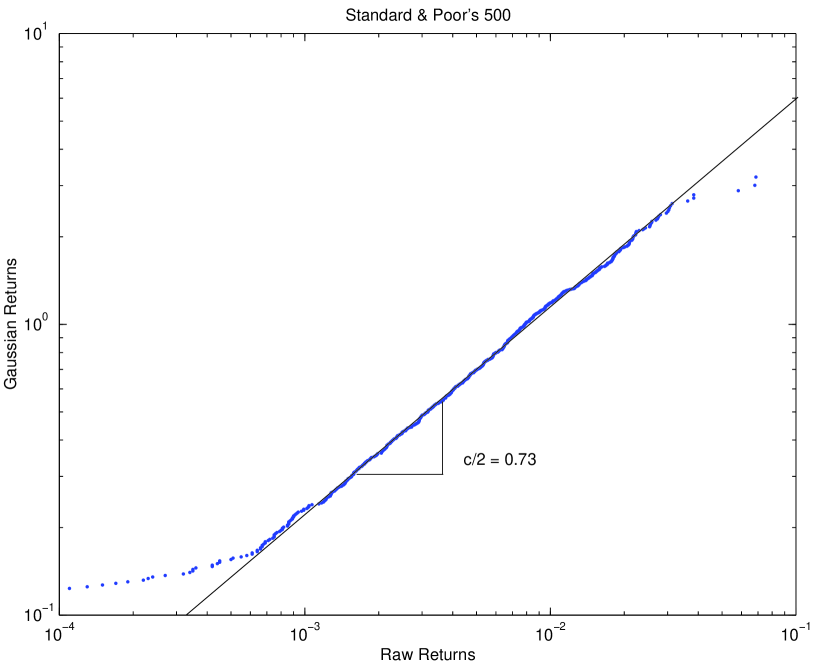
Figure 1: Graph of the Gaussianized Standard & Poor’s 500 index returns versus its raw returns, during the time interval from January 03, 1995 to December 29, 2000 for the negative tail of the distribution.

In what follows, we will assume that the marginal probability distributions of returns follow modified Weibull distributions. Figure 1 shows the (negative) “Gaussianized” returns $Y$ defined in (6) of the Standard and Poor’s 500 index versus the raw returns $X$ over the time interval from January 03, 1995 to December 29, 2000. With such a representation, the modified-Weibull distributions are qualified by a power law of exponent $c/2$, by definition 1. The double logarithmic scales of figure 1 clearly shows a straight line over an extended range of data, qualifying a power law relationship. An accurate determination of the parameters $(\chi,c)$ can be performed by maximum likelihood estimation [S2000, pp 160-162]. However, note that, in the tail, the six most extreme points significantly deviate from the modified-Weibull description. Such an anomalous behavior of the most extreme returns can be probably be associated with the notion of “outliers” introduced by JS98 JS98,JS02 and associated with behavioral and crowd phenomena during turbulent market phases.

The modified Weibull distributions defined here are of interest for financial purposes and specifically for portfolio and risk management, since they offer a flexible parametric representation of asset returns distribution either in a conditional or an unconditional framework, depending on the standpoint prefered by manager. The rest of the paper uses this family of distributions.

1.2 Tail equivalence for distribution functions

An interesting feature of the modified Weibull distributions, as we will see in the next section, is to enjoy the property of asymptotic stability. Asymptotic stability means that, in the regime of large deviations, a sum of independent and identically distributed modified Weibull variables follows the same modified Weibull distribution, up to a rescaling.

Definition 2 (Tail equivalence)

Let $X$ and $Y$ be two random variables with distribution function $F$ and $G$ respectively.

$X$ and $Y$ are said to be equivalent in the upper tail if and only if there exists $\lambda_{+}\in(0,\infty)$ such that

$$\lim_{x\rightarrow+\infty}\frac{1-F(x)}{1-G(x)}=\lambda_{+}.$$ (10)

Similarly, $X$ and $Y$ are said equivalent in the lower tail if and only if there exists $\lambda_{-}\in(0,\infty)$ such that

$$\lim_{x\rightarrow-\infty}\frac{F(x)}{G(x)}=\lambda_{-}.$$ (11)

$\square$

Applying l’Hospital’s rule, this gives immediately the following corollary:

Corollary 1

Let $X$ and $Y$ be two random variables with densities functions $f$ and $g$ respectively. $X$ and $Y$ are equivalent in the upper (lower) tail if and only if

$$\lim_{x\rightarrow\pm\infty}\frac{f(x)}{g(x)}=\lambda_{\pm},~{}~{}~{}\lambda_{\pm}\in(0,\infty).$$ (12)

$\square$

1.3 The Gaussian copula

We recall only the basic properties about copulas and refer the interested reader to [Nelsen], for instance, for more information. Let us first give the definition of a copula of $n$ random variables.

Definition 3 (Copula)

A function $C$ : $[0,1]^{n}\longrightarrow[0,1]$ is a $n$-copula if it enjoys the following properties :

• $\forall u\in[0,1]$, $C(1,\cdots,1,u,1\cdots,1)=u$ ,

• $\forall u_{i}\in[0,1]$, $C(u_{1},\cdots,u_{n})=0$ if at least one of the $u_{i}$ equals zero ,

• $C$ is grounded and $n$-increasing, i.e., the $C$-volume of every boxes whose vertices lie in $[0,1]^{n}$ is positive. $\square$

The fact that such copulas can be very useful for representing multivariate distributions with arbitrary marginals is seen from the following result.

Theorem 1 (Sklar’s Theorem)

Given an $n$-dimensional distribution function $F$ with continuous marginal distributions $F_{1},\cdots,F_{n}$, there exists a unique $n$-copula $C$ : $[0,1]^{n}\longrightarrow[0,1]$ such that :

$$F(x_{1},\cdots,x_{n})=C(F_{1}(x_{1}),\cdots,F_{n}(x_{n}))~{}.$$ (13)

$\square$

This theorem provides both a parameterization of multivariate distributions and a construction scheme for copulas. Indeed, given a multivariate distribution $F$ with margins $F_{1},\cdots,F_{n}$, the function

$$C(u_{1},\cdots,u_{n})=F\left(F_{1}^{-1}(u_{1}),\cdots,F_{n}^{-1}(u_{n})\right)$$ (14)

is automatically a $n$-copula. Applying this theorem to the multivariate Gaussian distribution, we can derive the so-called Gaussian copula.

Definition 4 (Gaussian copula)

Let $\Phi$ denote the standard Normal distribution and $\Phi_{V,n}$ the $n$-dimensional Gaussian distribution with correlation matrix ${\bf V}$. Then, the Gaussian $n$-copula with correlation matrix ${\bf V}$ is

$$C_{V}(u_{1},\cdots,u_{n})=\Phi_{V,n}\left(\Phi^{-1}(u_{1}),\cdots,\Phi^{-1}(u_{n})\right)~{},$$ (15)

whose density

$$c_{V}(u_{1},\cdots,u_{n})=\frac{\partial C_{V}(u_{1},\cdots,u_{n})}{\partial u_{1}\cdots\partial u_{n}}$$ (16)

reads

$$c_{V}(u_{1},\cdots,u_{n})=\frac{1}{\sqrt{\det{\bf V}}}\exp\left(-\frac{1}{2}y_{(u)}^{t}({\bf V}^{-1}-\mbox{Id})y_{(u)}\right)$$ (17)

with $y_{k}(u)=\Phi^{-1}(u_{k})$. Note that theorem 1 and equation (14) ensure that $C_{V}(u_{1},\cdots,u_{n})$ in equation (15) is a copula. $\square$

It can be shown that the Gaussian copula naturally arises when one tries to determine the dependence between random variables using the principle of entropy maximization [Rao, Sornette1, for instance]. Its pertinence and limitations for modeling the dependence between assets returns has been tested by MS01, who show that in most cases, this description of the dependence can be considered satisfying, specially for stocks, provided that one does not consider too extreme realizations [MS_risk, MS_ext, zeevi].

2 Portfolio wealth distribution for several dependence structures

2.1 Portfolio wealth distribution for independent assets

Let us first consider the case of a portfolio made of independent assets. This limiting (and unrealistic) case is a mathematical idealization which provides a first natural benchmark of the class of portolio return distributions to be expected. Moreover, it is generally the only case for which the calculations are analytically tractable. For such independepent assets distributed with the modified Weibull distributions, the following results prove the asymptotic stability of this set of distributions:

Theorem 2 (Tail equivalence for i.i.d modified Weibull random variables)

Let $X_{1},X_{2},\cdots,X_{N}$ be $N$ independent and identically ${\cal W}(c,\chi)$-distributed random variables. Then, the variable

$$S_{N}=X_{1}+X_{2}+\cdots+X_{N}$$ (18)

is equivalent in the lower and upper tail to $Z\sim{\cal W}(c,\hat{\chi})$, with

$$\hat{\chi} = N^{\frac{c-1}{c}}\chi,~{}~{}~{}c>1,$$ (19)

$$\hat{\chi} = \chi,~{}~{}~{}~{}~{}~{}~{}~{}~{}~{}~{}~{}~{}c\leq 1.$$ (20)

$\square$

This theorem is a direct consequence of the theorem stated below and is based on the result given by FS97 for $c>1$ and on general properties of sub-exponential distributions when $c\leq 1$.

Theorem 3 (Tail equivalence for weighted sums of independent variables)

Let $X_{1},X_{2},\cdots,X_{N}$ be $N$ independent and identically ${\cal W}(c,\chi)$-distributed random variables. Let $w_{1}$, $w_{2},\cdots,w_{N}$ be $N$ non-random real coefficients. Then, the variable

$$S_{N}=w_{1}X_{1}+w_{2}X_{2}+\cdots+w_{N}X_{N}$$ (21)

is equivalent in the upper and the lower tail to $Z\sim{\cal W}(c,\hat{\chi})$ with

$$\hat{\chi} = \left(\sum_{i=1}^{N}|w_{i}|^{\frac{c}{c-1}}\right)^{\frac{c-1}{c}}\cdot\chi,~{}~{}~{}~{}~{}~{}~{}~{}~{}~{}c>1,$$ (22)

$$\hat{\chi} = \max_{i}\{|w_{1}|,|w_{2}|,\cdots,|w_{N}|\},~{}~{}~{}c\leq 1.$$ (23)

$\square$

The proof of this theorem is given in appendix A.

Corollary 2

Let $X_{1},X_{2},\cdots,X_{N}$ be $N$ independent random variables such that $X_{i}\sim{\cal W}(c,\chi_{i})$. Let $w_{1}$, $w_{2},\cdots,w_{N}$ be $N$ non-random real coefficients. Then, the variable

$$S_{N}=w_{1}X_{1}+w_{2}X_{2}+\cdots+w_{N}X_{N}$$ (24)

is equivalent in the upper and the lower tail to $Z\sim{\cal W}(c,\hat{\chi})$ with

$$\hat{\chi} = \left(\sum_{i=1}^{N}|w_{i}\chi_{i}|^{\frac{c}{c-1}}\right)^{\frac{c-1}{c}}~{},~{}~{}~{}c>1,$$ (25)

$$\hat{\chi} = \max_{i}\{|w_{1}\chi_{1}|,|w_{2}\chi_{2}|,\cdots,|w_{N}\chi_{N}|\},~{}~{}~{}c\leq 1.$$ (26)

$\square$

The proof of the corollary is a straightforward application of theorem 3. Indeed, let $Y_{1},Y_{2},\cdots,Y_{N}$ be $N$ independent and identically ${\cal W}(c,1)$-distributed random variables. Then,

$$(X_{1},X_{2},\cdots,X_{N})\stackrel{{\scriptstyle d}}{{=}}(\chi_{1}Y_{1},\chi_{2}Y_{2},\cdots,\chi_{N}Y_{N}),$$ (27)

which yields

$$S_{N}\stackrel{{\scriptstyle d}}{{=}}w_{1}\chi_{1}\cdot Y_{1}+w_{2}\chi_{2}\cdot Y_{2}+\cdots+w_{N}\chi_{N}\cdot Y_{N}~{}.$$ (28)

Thus, applying theorem 3 to the i.i.d variables $Y_{i}$’s with weights $w_{i}\chi_{i}$ leads to corollary 2.

2.2 Portfolio wealth distribution for comonotonic assets

The case of comonotonic assets is of interest as the limiting case of the strongest possible dependence between random variables. By definition,

Definition 5 (Comonotonicity)

the variables $X_{1},X_{2},\cdots,X_{N}$ are comonotonic if and only if there exits a random variable $U$ and non-decreasing functions $f_{1},f_{2},\cdots,f_{N}$ such that

$$(X_{1},X_{2},\cdots,X_{N})\stackrel{{\scriptstyle d}}{{=}}(f_{1}(U),f_{2}(U),\cdots,f_{N}(U)).$$ (29)

$\square$

In terms of copulas, the comonotonicity can be expressed by the following form of the copula

$$C(u_{1},u_{2},\cdots,u_{N})=\min(u_{1},u_{2},\cdots,u_{N})~{}.$$ (30)

This expression is known as the Fréchet-Hoeffding upper bound for copulas [Nelsen, for instance]. It would be appealing to think that estimating the Value-at-Risk under the comonotonicity assumption could provide an upper bound for the Value-at-Risk. However, it turns out to be wrong, due –as we shall see in the sequel– to the lack of coherence (in the sense of Artzner) of the Value-at-Risk, in the general case. Notwithstanding, an upper and lower bound can always be derived for the Value-at-Risk [EHJ02]. But in the present situation, where we are only interested in the class of modified Weibull distributions with a Gaussian copula, the VaR derived under the comonoticity assumption will actually represent the upper bound (at least for the VaR calculated at sufficiently hight confidence levels).

Theorem 4 (Tail equivalence for a sum of comonotonic random variables)

Let $X_{1},X_{2},\cdots,X_{N}$ be $N$ comonotonic random variables such that $X_{i}\sim{\cal W}(c,\chi_{i})$. Let $w_{1},w_{2},\cdots,w_{N}$ be $N$ non-random real coefficients. Then, the variable

$$S_{N}=w_{1}X_{1}+w_{2}X_{2}+\cdots+w_{N}X_{N}$$ (31)

is equivalent in the upper and the lower tail to $Z\sim{\cal W}(c,\hat{\chi})$ with

$$\hat{\chi}=\sum_{i}w_{i}\chi_{i}~{}.$$ (32)

$\square$

The proof is obvious since, under the assumption of comonotonicity, the portfolio wealth $S$ is given by

$$S=\sum_{i}w_{i}\cdot X_{i}\stackrel{{\scriptstyle d}}{{=}}\sum_{i=1}^{N}w_{i}\cdot f_{i}(U),$$ (33)

and for modified Weibull distributions, we have

$$f_{i}(\cdot)=\mbox{sgn}(\cdot)~{}\chi_{i}\left(\frac{|\cdot|}{\sqrt{2}}\right)^{2/c_{i}},$$ (34)

in the symmetric case while $U$ is a Gaussian random variable. If, in addition, we assume that all assets have the same exponent $c_{i}=c$, it is clear that $S\sim{\cal W}(c,\hat{\chi})$ with

$$\hat{\chi}=\sum_{i}w_{i}\chi_{i}.$$ (35)

It is important to note that this relation is exact and not asymptotic as in the case of independent variables.

When the exponents $c_{i}$’s are different from an asset to another, a similar result holds, since we can still write the inverse cumulative function of $S$ as

$$F_{S}^{-1}(p)=\sum_{i=1}^{N}w_{i}F_{X_{i}}^{-1}(p),~{}~{}~{}~{}~{}p\in(0,1),$$ (36)

which is the property of additive comonotonicity of the Value-at-Risk. Let us then sort the $X_{i}$’s such that $c_{1}=c_{2}=\cdots=c_{p}<c_{p+1}\leq\cdots\leq c_{N}$. We immediately obtain that $S$ is equivalent in the tail to $Z\sim{\cal W}(c_{1},\hat{\chi})$, where

$$\hat{\chi}=\sum_{i=1}^{p}w_{i}\chi_{i}.$$ (37)

In such a case, only the assets with the fatest tails contributes to the behavior of the sum in the large deviation regime.

2.3 Portfolio wealth under the Gaussian copula hypothesis

2.3.1 Derivation of the multivariate distribution with a Gaussian copula and modified Weibull margins

An advantage of the class of modified Weibull distributions (7) is that the transformation into a Gaussian, and thus the calculation of the vector ${\bf y}$ introduced in definition 1, is particularly simple. It takes the form

$$y_{k}=\mbox{sgn}(x_{k})~{}\sqrt{2}~{}\left(\frac{|x_{k}|}{\chi_{k}}\right)^{\frac{c_{k}}{2}},$$ (38)

where $y_{k}$ is normally distributed . These variables $Y_{i}$ then allow us to obtain the covariance matrix ${\bf V}$ of the Gaussian copula :

$$V_{ij}=2\cdot{\rm E}\left[\mbox{sgn}(x_{i}x_{j})\left(\frac{|x_{i}|}{\chi_{i}}\right)^{\frac{c_{i}}{2}}\left(\frac{|x_{j}|}{\chi_{j}}\right)^{\frac{c_{j}}{2}}\right]\;,$$ (39)

which always exists and can be efficiently estimated. The multivariate density $P({\bf x})$ is thus given by:

$$P(x_{1},\cdots,x_{N}) = c_{V}(x_{1},x_{2},\cdots,x_{N})~{}\prod_{i=1}^{N}p_{i}(x_{i})$$ (40)

$$= \frac{1}{2^{N}\pi^{N/2}\sqrt{V}}\prod_{i=1}^{N}\frac{c_{i}|x_{i}|^{c/2-1}}{\chi_{i}^{c/2}}\exp\left[-\sum_{i,j}V_{ij}^{-1}\left(\frac{|x_{i}|}{\chi_{i}}\right)^{c/2}\left(\frac{|x_{j}|}{\chi_{j}}\right)^{c/2}\right]~{}.$$ (41)

Obviously, similar transforms hold, mutatis mutandis, for the asymmetric case (8,9).

2.3.2 Asymptotic distribution of a sum of modified Weibull variables with the same exponent $c>1$

We now consider a portfolio made of dependent assets with pdf given by equation (41) or its asymmetric generalization. For such distributions of asset returns, we obtain the following result

Theorem 5 (Tail equivalence for a sum of dependent random variables)

Let $X_{1},X_{2},\cdots,X_{N}$ be $N$ random variables with a dependence structure described by the Gaussian copula with correlation matrix ${\bf V}$ and such that each $X_{i}\sim{\cal W}(c,\chi_{i})$. Let $w_{1},w_{2},\cdots,w_{N}$ be $N$ (positive) non-random real coefficients. Then, the variable

$$S_{N}=w_{1}X_{1}+w_{2}X_{2}+\cdots+w_{N}X_{N}$$ (42)

is equivalent in the upper and the lower tail to $Z\sim{\cal W}(c,\hat{\chi})$ with

$$\hat{\chi}=\left(\sum_{i}w_{i}\chi_{i}\sigma_{i}\right)^{\frac{c-1}{c}},$$ (43)

where the $\sigma_{i}$’s are the unique (positive) solution of

$$\sum_{i}V_{ik}^{-1}{\sigma_{i}}^{c/2}=w_{k}\chi_{k}~{}\sigma_{k}^{1-c/2}~{},~{}~{}~{}~{}~{}~{}~{}~{}~{}~{}~{}~{}\forall k~{}.$$ (44)

$\square$

The proof of this theorem follows the same lines as the proof of theorem 3. We thus only provide a heuristic derivation of this result in appendix B. Equation (44) is equivalent to

$$\sum_{k}V_{ik}~{}w_{k}\chi_{k}~{}{\sigma_{k}}^{1-c/2}={\sigma_{i}}^{c/2}~{},~{}~{}~{}~{}~{}~{}~{}~{}~{}~{}~{}~{}\forall i~{}.$$ (45)

which seems more attractive since it does not require the inversion of the correlation matrix. In the special case where ${\bf V}$ is the identity matrix, the variables $X_{i}$’s are independent so that equation (43) must yield the same result as equation (22). This results from the expression of $\sigma_{k}=(w_{k}\chi_{k})^{\frac{1}{c-1}}$ valid in the independent case. Moreover, in the limit where all entries of V equal one, we retrieve the case of comonotonic assets. Obviously, ${\bf V}^{-1}$ does not exist for comonotonic assets and the derivation given in appendix B does not hold, but equation (45) remains well-defined and still has a unique solution $\sigma_{k}=(\sum w_{k}\chi_{k})^{\frac{1}{c-1}}$ which yields the scale factor given in theorem 4.

2.4 Summary

In the previous sections, we have shown that the wealth distribution $F_{S}(x)$ of a portfolio made of assets with modified Weibull distributions with the same exponent $c$ remains equivalent in the tail to a modified Weibull distribution ${\cal W}(c,\hat{\chi})$. Specifically,

$$F_{S}(x)\sim\lambda_{-}~{}F_{Z}(x)~{},$$ (46)

when $x\rightarrow-\infty$, and where $Z\sim{\cal W}(c,\hat{\chi})$. Expression (46) defines the proportionality factor or weight $\lambda_{-}$ of the negative tail of the portfolio wealth distribution $F_{S}(x)$. Table 1 summarizes the value of the scale parameter $\hat{\chi}$ for the different types of dependence we have studied. In addition, we give the value of the coefficient $\lambda_{-}$, which may also depend on the weights of the assets in the portfolio in the case of dependent assets.

	$\hat{\chi}$	$\lambda_{-}$
	$\left(\sum_{i=1}^{N}|w_{i}\chi_{i}|^{\frac{c}{c-1}}\right)^{\frac{c-1}{c}}$, $c>1$	$\left[\frac{c}{2(c-1)}\right]^{\frac{N-1}{2}}$
Independent Assets
	$\max\{|w_{1}\chi_{1}|,\cdots,|w_{N}\chi_{N}|\}$, $c\leq 1$	Card $\{|w_{i}\chi_{i}|=\max_{j}\{\ |w_{j}\chi_{j}|\}\}$
Comonotonic Assets	$\sum_{i=1}^{N}w_{i}\chi_{i}$	$1$
Gaussian copula	$\left(\sum_{i}w_{i}\chi_{i}\sigma_{i}\right)^{\frac{c-1}{c}}$ , $c>1$	see appendix B

Table 1: Summary of the various scale factors obtained for different distribution of asset returns.

3 Value-at-Risk

3.1 Calculation of the VaR

We consider a portfolio made of $N$ assets with all the same exponent $c$ and scale parameters $\chi_{i}$, $i\in\{1,2,\cdots,N\}$. The weight of the i^th asset in the portfolio is denoted by $w_{i}$. By definition, the Value-at-Risk at the loss probability $\alpha$, denoted by $\mbox{VaR}_{\alpha}$, is given , for a continuous distribution of profit and loss, by

$$\Pr\{W(\tau)-W(0)<-\mbox{VaR}_{\alpha}\}=\alpha,$$ (47)

which can be rewritten as

$$\Pr\left\{S<-\frac{\mbox{VaR}_{\alpha}}{W(0)}\right\}=\alpha.$$ (48)

In this expression, we have assumed that all the wealth is invested in risky assets and that the risk-free interest rate equals zero, but it is easy to reintroduce it, if necessary. It just leads to discount ${\rm VaR}_{\alpha}$ by the discount factor ${1/(1+\mu_{0})}$, where $\mu_{0}$ denotes the risk-free interest rate.

Now, using the fact that $F_{S}(x)\sim\lambda_{-}~{}F_{Z}(x)$, when $x\rightarrow-\infty$, and where $Z\sim{\cal W}(c,\hat{\chi})$, we have

$$\frac{1}{\lambda_{-}}~{}\Pr\left\{S<-\frac{\mbox{VaR}_{\alpha}}{W(0)}\right\}\simeq 1-\Phi\left(\sqrt{2}\left(\frac{\mbox{VaR}_{\alpha}}{W(0)~{}\hat{\chi}}\right)^{c/2}\right),$$ (49)

as $\mbox{VaR}_{\alpha}$ goes to infinity, which allows us to obtain a closed expression for the asymptotic Value-at-Risk with a loss probability $\alpha$:

$$\mbox{VaR}_{\alpha} \simeq W(0)~{}\frac{\hat{\chi}}{2^{1/c}}\left[\Phi^{-1}\left(1-\frac{\alpha}{\lambda_{-}}\right)\right]^{2/c},$$ (50)

$$\simeq \xi(\alpha)^{2/c}~{}W(0)\cdot\hat{\chi},$$ (51)

where the function $\Phi(\cdot)$ denotes the cumulative Normal distribution function and

$$\xi(\alpha)\equiv\frac{1}{2}\Phi^{-1}\left(1-\frac{\alpha}{\lambda_{-}}\right)~{}.$$ (52)

In the case where a fraction $w_{0}$ of the total wealth is invested in the risk-free asset with interest rate $\mu_{0}$, the previous equation simply becomes

$$\mbox{VaR}_{\alpha}\simeq\xi(\alpha)^{2/c}~{}(1-w_{0})\cdot W(0)\cdot\hat{\chi}-w_{0}W(0)\mu_{0}.$$ (53)

Due to the convexity of the scale parameter $\hat{\chi}$, the VaR is itself convex and therefore sub-additive. Thus, for this set of distributions, the VaR becomes coherent when the considered quantiles are sufficiently small.

The Expected-Shortfall $ES_{\alpha}$, which gives the average loss beyond the VaR at probability level $\alpha$, is also very easily computable:

$$ES_{\alpha} = \frac{1}{\alpha}\int_{0}^{\alpha}{\rm VaR}_{u}~{}du$$ (54)

$$= \zeta(\alpha)(1-w_{0})\cdot W(0)\cdot\hat{\chi}-w_{0}W(0)\mu_{0},$$ (55)

where $\zeta(\alpha)=\frac{1}{\alpha}\int_{0}^{\alpha}\xi(u)^{2/c}~{}du~{}$. Thus, the Value-at-Risk, the Expected-Shortfall and in fact any downside risk measure involving only the far tail of the distribution of returns are entirely controlled by the scale parameter $\hat{\chi}$. We see that our set of multivariate modified Weibull distributions enjoy, in the tail, exactly the same properties as the Gaussian distributions, for which, all the risk measures are controlled by the standard deviation.

3.2 Typical recurrence time of large losses

Let us translate these formulas in intuitive form. For this, we define a Value-at-Risk $\mbox{VaR}^{*}$ which is such that its typical frequency is $1/T_{0}$. $T_{0}$ is by definition the typical recurrence time of a loss larger than $\mbox{VaR}^{*}$. In our present example, we take $T_{0}$ equals $1$ year for example, i.e., $\mbox{VaR}^{*}$ is the typical annual shock or crash. Expression (49) then allows us to predict the recurrence time $T$ of a loss of amplitude VaR equal to $\beta$ times this reference value $\mbox{VaR}^{*}$:

$$\ln\left(\frac{T}{T_{0}}\right)\simeq(\beta^{c}-1)\left(\frac{\mbox{VaR}^{*}}{W(0)~{}\hat{\chi}}\right)^{c}+{\cal O}(\ln\beta)~{}.$$ (56)

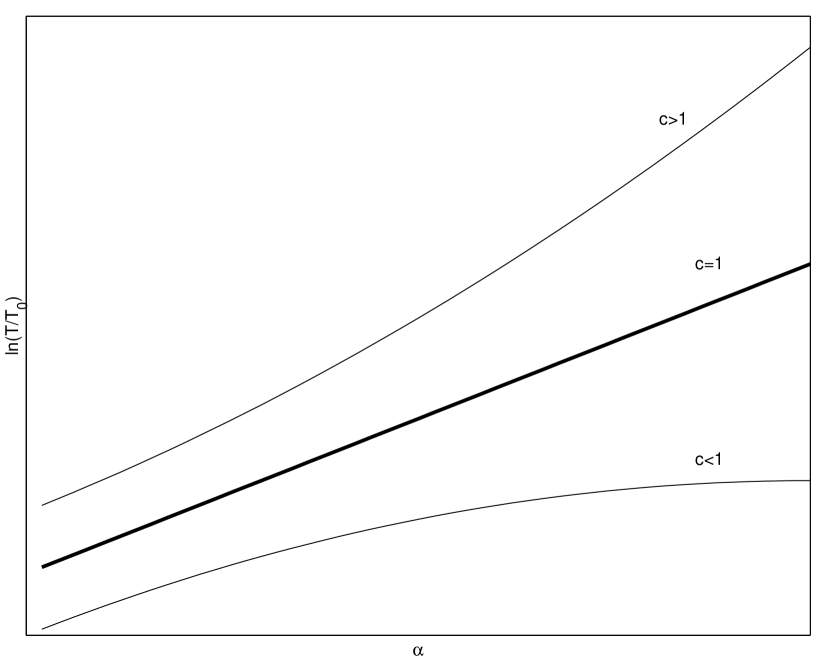
Figure 2: Logarithm $\ln\left(\frac{T}{T_{0}}\right)$ of the ratio of the recurrence time $T$ to a reference time $T_{0}$ for the recurrence of a given loss $VaR$ as a function of $\beta$ defined by $\beta=\frac{\rm VaR}{{\rm VaR}^{*}}$. ${\rm VaR}^{*}$ (resp. ${\rm VaR}$) is the Value-at-Risk over a time interval $T_{0}$ (resp. $T$).

Figure 2 shows $\ln\frac{T}{T_{0}}$ versus $\beta$. Observe that $T$ increases all the more slowly with $\beta$, the smaller is the exponent $c$. This quantifies our expectation that large losses occur more frequently for the “wilder” sub-exponential distributions than for super-exponential ones.

4 Optimal portfolios

In this section, we present our results on the problem of the efficient portfolio allocation for asset distributed according to modified Weibull distributions with the different dependence structures studied in the previous sections. We focus on the case when all asset modified Weibull distributions have the same exponent $c$, as it provides the richest and more varied situation. When this is not the case and the assets have different exponents $c_{i}$, $i=1,...,N$, the asymptotic tail of the portfolio return distribution is dominated by the asset with the heaviest tail. The largest risks of the portfolio are thus controlled by the single most risky asset characterized by the smallest exponent $c$. Such extreme risk cannot be diversified away. In such a case, for a risk-averse investor, the best strategy focused on minimizing the extreme risks consists in holding only the asset with the thinnest tail, i.e., with the largest exponent $c$.

4.1 Portfolios with minimum risk

Let us consider first the problem of finding the composition of the portfolio with minimum risks, where the risks are measured by the Value-at-Risk. We consider that short sales are not allowed, that the risk free interest rate equals zero and that all the wealth is invested in stocks. This last condition is indeed the only interesting one since allowing to invest in a risk-free asset would automatically give the trivial solution in which the minimum risk portfolio is completely invested in the risk-free asset.

The problem to solve reads:

$$\mbox{VaR}_{\alpha}^{*}=\min\mbox{VaR}_{\alpha}=\xi(\alpha)^{2/c}~{}W(0)\cdot\min\hat{\chi}$$ (57)

$$\sum_{i=1}^{N}w_{i}=1$$ (58)

$$w_{i}\geq 0~{}~{}~{}~{}\forall i.$$ (59)

In some cases (see table 1), the prefactor $\xi(\alpha)$ defined in (52) also depends on the weight $w_{i}$’s through $\lambda_{-}$ defined in (46). But, its contribution remains subdominant for the large losses. This allows to restrict the minimization to $\hat{\chi}$ instead of $\xi(\alpha)^{2/c}\cdot\hat{\chi}$.

4.1.1 Case of independent assets

“Super-exponential” portfolio ($c>1$)

Consider assets distributed according to modified Weibull distributions with the same exponent $c>1$. The Value-at-Risk is given by

$$\mbox{VaR}_{\alpha}=\xi(\alpha)^{2/c}~{}W(0)\cdot\left(\sum_{i=1}^{N}|w_{i}\chi_{i}|^{\frac{c}{c-1}}\right)^{\frac{c-1}{2}}~{},$$ (60)

Introducing the Lagrange multiplier $\lambda$, the first order condition yields

$$\frac{\partial\hat{\chi}}{\partial w_{i}}=\frac{\lambda}{\xi(\alpha)~{}W(0)}~{}~{}~{}~{}\forall i,$$ (61)

and the composition of the minimal risk portfolio is

$${w_{i}}^{*}=\frac{\chi_{i}^{-c}}{\sum_{j}\chi_{j}^{-c}}$$ (62)

which satistifies the positivity of the Hessian matrix $H_{jk}=\left.\frac{\partial^{2}\hat{\chi}}{\partial w_{j}\partial w_{k}}\right|_{\{w_{i}^{*}\}}$ (second order condition).

The minimal risk portfolio is such that

$$\mbox{VaR}_{\alpha}^{*}=\frac{\xi(\alpha)^{2/c}~{}W(0)}{\left(\sum_{i}\chi_{j}^{-c}\right)^{\frac{1}{c}}}~{},~{}~{}~{}~{}~{}\mu^{*}=\frac{\sum_{i}\chi_{i}^{-c}\mu_{i}}{\sum_{j}\chi_{j}^{-c}}~{},$$ (63)

where $\mu_{i}$ is the return of asset $i$ and $\mu^{*}$ is the return of the minimum risk portfolio.

sub-exponential portfolio ($c\leq 1$)

Consider assets distributed according to modified Weibull distributions with the same exponent $c<1$. The Value-at-Risk is now given by

$$\mbox{VaR}_{\alpha}=\xi(\alpha)^{c/2}~{}W(0)\cdot\max\{|w_{1}\chi_{1}|,\cdots,|w_{N}\chi_{N}|\}.$$ (64)

Since the weights $w_{i}$ are positive, the modulus appearing in the argument of the max() function can be removed. It is easy to see that the minimum of $\mbox{VaR}_{\alpha}$ is obtained when all the $w_{i}\chi_{i}$’s are equal, provided that the constraint $\sum w_{i}=1$ can be satisfied. Indeed, let us start with the situation where

$$w_{1}\chi_{1}=w_{2}\chi_{2}=\cdots=w_{N}\chi_{N}~{}.$$ (65)

Let us decrease the weight $w_{1}$. Then, $w_{1}\chi_{1}$ decreases with respect to the initial maximum situation (65) but, in order to satisfy the constraint $\sum_{i}w_{i}=1$, at least one of the other weights $w_{j}$, $j\geq 2$ has to increase, so that $w_{j}\chi_{j}$ increases, leading to a maximum for the set of the $w_{i}\chi_{i}$’s greater than in the initial situation where (65) holds. Therefore,

$$w_{i}^{*}=\frac{A}{\chi_{i}}~{},~{}~{}~{}~{}\forall i,$$ (66)

and the constraint $\sum_{i}w_{i}=1$ yields

$$A=\frac{1}{\sum_{i}\chi_{i}^{-1}},$$ (67)

and finally

$$w_{i}^{*}=\frac{\chi_{i}^{-1}}{\sum_{j}\chi_{j}^{-1}}~{},~{}~{}~{}~{}~{}\mbox{VaR}_{\alpha}^{*}=\frac{\xi(\alpha)^{c/2}~{}W(0)}{\sum_{i}\chi_{i}^{-1}},~{}~{}~{}~{}~{}~{}~{}~{}\mu^{*}=\frac{\sum_{i}\chi_{i}^{-1}\mu_{i}}{\sum_{j}\chi_{j}^{-1}}~{}.$$ (68)

The composition of the optimal portfolio is continuous in $c$ at the value $c=1$. This is the consequence of the continuity as a function of $c$ at $c=1$ of the scale factor $\hat{\chi}$ for a sum of independent variables. In this regime $c\leq 1$, the Value-at-Risk increases as $c$ decreases only through its dependence on the prefactor $\xi(\alpha)^{2/c}$ since the scale factor $\hat{\chi}$ remains constant.

4.1.2 Case of comonotonic assets

For comonotonic assets, the Value-at-Risk is

$$\mbox{VaR}_{\alpha}=\xi(\alpha)^{c/2}~{}W(0)\cdot\sum_{i}w_{i}\chi_{i}$$ (69)

which leads to a very simple linear optimization problem. Indeed, denoting $\chi_{1}=\min\{\chi_{1},$ $\chi_{2},\cdots,\chi_{N}\}$, we have

$$\sum_{i}w_{i}\chi_{i}\geq\chi_{1}~{}\sum_{i}w_{i}=\chi_{1},$$ (70)

which proves that the composition of the optimal portfolio is $w_{1}^{*}=1,w_{i}^{*}=0~{}~{}i\geq 2$ leading to

$$\mbox{VaR}_{\alpha}^{*}=\xi(\alpha)^{c/2}~{}W(0)\chi_{1},~{}~{}~{}~{}\mu^{*}=\mu_{1}.$$ (71)

This result is not surprising since all assets move together. Thus, the portfolio with minimum Value-at-Risk is obtained when only the less risky asset, i.e., with the smallest scale factor $\chi_{i}$, is held. In the case where there is a degeneracy in the smallest $\chi$ of order $p$ ($\chi_{1}=\chi_{2}=...=\chi_{p}=\min\{\chi_{1},\chi_{2},\cdots,\chi_{N}\}$), the optimal choice lead to invest all the wealth in the asset with the larger expected return $\mu_{j}$, $j\in\{1,\cdots,p\}$. However, in an efficient market with rational agents, such an opportunity should not exist since the same risk embodied by $\chi_{1}=\chi_{2}=...=\chi_{p}$ should be remunerated by the same return $\mu_{1}=\mu_{2}=...=\mu_{p}$.

4.1.3 Case of assets with a Gaussian copula

In this situation, we cannot solve the problem analytically. We can only assert that the miminization problem has a unique solution, since the function $\mbox{VaR}_{\alpha}(\{w_{i}\})$ is convex. In order to obtain the composition of the optimal portfolio, we need to perform the following numerical analysis.

It is first needed to solve the set of equations $\sum_{i}V_{ij}^{-1}\sigma_{i}^{c/2}=w_{j}\chi_{j}\sigma_{j}^{1-c/2}$ or the equivalent set of equations given by (45), which can be performed by Newton’s algorithm. Then one have the minimize the quantity $\sum w_{i}\chi_{i}\sigma_{i}(\{w_{i}\})$. To this aim, one can use the gradient algorithm, which requires the calculation of the derivatives of the $\sigma_{i}$’s with respect to the $w_{k}$’s. These quantities are easily obtained by solving the linear set of equations

$$\frac{c}{2}\cdot\sum_{i}V_{ij}^{-1}\sigma_{i}^{\frac{c}{2}-1}\sigma_{j}^{\frac{c}{2}-1}\frac{\partial\sigma_{i}}{\partial w_{k}}+\left(\frac{c}{2}-1\right)w_{j}\chi_{j}\frac{1}{\sigma_{j}}\frac{\partial\sigma_{j}}{\partial w_{k}}=\chi_{j}\cdot\delta_{jk}.$$ (72)

Then, the analytical solution for independent assets or comonotonic assets can be used to initialize the minimization algorithm with respect to the weights of the assets in the portfolio.

4.2 VaR-efficient portfolios

We are now interested in portfolios with minimum Value-at-risk, but with a given expected return $\mu=\sum_{i}w_{i}\mu_{i}$. We will first consider the case where, as previously, all the wealth is invested in risky assets and we then will discuss the consequences of the introduction of a risk-free asset in the portfolio.

4.2.1 Portfolios without risky asset

When the investors have to select risky assets only, they have to solve the following minimization problem:

$$\mbox{VaR}_{\alpha}^{*}=\min\mbox{VaR}_{\alpha}=\xi(\alpha)~{}W(0)\cdot\min\hat{\chi}$$ (73)

$$\sum_{i=1}^{N}w_{i}\mu_{i}=\mu$$ (74)

$$\sum_{i=1}^{N}w_{i}=1$$ (75)

$$w_{i}\geq 0~{}~{}~{}~{}\forall i.$$ (76)

In contrast with the research of the minimum risk portfolios where analytical results have been derived, we need here to use numerical methods in every situation. In the case of super-exponential portfolios, with or without dependence between assets, the gradient method provides a fast and easy to implement algorithm, while for sub-exponential portfolios or portfolios made of comonotonic assets, one has to use the simplex method since the minimization problem is then linear.

Thus, although not as convenient to handle as analytical results, these optimization problems remain easy to manage and fast to compute even for large portfolios.

4.2.2 Portfolios with risky asset

When a risk-free asset is introduced in the portfolio, the expression of the Value-at-Risk is given by equation (53), the minimization problem becomes

$$\mbox{VaR}_{\alpha}^{*}=\min\xi(\alpha)^{2/c}~{}(1-w_{0})\cdot W(0)\cdot\hat{\chi}-w_{0}W(0)\mu_{0}$$ (77)

$$\sum_{i=1}^{N}w_{i}\mu_{i}=\mu$$ (78)

$$\sum_{i=1}^{N}w_{i}=1$$ (79)

$$w_{i}\geq 0~{}~{}~{}~{}\forall i.$$ (80)

When the risk-free interest rate $\mu_{0}$ is non zero, we have to use the same numerical methods as above to solve the problem. However, if we assume that $\mu_{0}=0$, the problem becomes amenable analytically. Its Lagrangian reads

$${\cal L} = \xi(\alpha)^{2/c}~{}(1-w_{0})\cdot W(0)\cdot\hat{\chi}-\lambda_{1}\left(\sum_{i\neq 0}w_{i}\mu_{i}-\mu\right)-\lambda_{2}\left(\sum_{i=0}^{N}w_{i}-1\right),$$ (81)

$$= \xi(\alpha)^{2/c}~{}\left(\sum_{j\neq 0}w_{i}\right)\cdot W(0)\cdot\hat{\chi}-\lambda_{1}\left(\sum_{i\neq 0}w_{i}\mu_{i}-\mu\right),$$ (82)

which allows us to show that the weights of the optimal portfolio are

$$w_{i}^{*}=(1-w_{0})\cdot\frac{\hat{w}_{i}}{\sum_{j=1}^{N}\hat{w}_{j}}~{}~{}~{}~{}~{}~{}{\rm and}~{}~{}~{}~{}~{}~{}~{}\mbox{VaR}_{\alpha}^{*}=\frac{\xi(\alpha)^{2/c}~{}(1-w_{0})\cdot W(0)}{2}\cdot\mu,$$ (83)

where the $\hat{w}_{i}$’s are solution of the set of equations

$$\hat{\chi}+\left(\sum_{i=1}^{N}\hat{w}_{i}\right)\frac{\partial\hat{\chi}}{\partial\hat{w}_{i}}=\mu_{i}~{}.$$ (84)

Expression (83) shows that the efficient frontier is simply a straight line and that any efficient portfolio is the sum of two portfolios: a “riskless portfolio” in which a fraction $w_{0}$ of the initial wealth is invested and a portfolio with the remaining $(1-w_{0})$ of the initial wealth invested in risky assets. This provides another example of the two funds separation theorem. A CAPM then holds, since equation (84) together with the market equilibrium assumption yields the proportionality between any stock return and the market return. However, these three properties are rigorously established only for a zero risk-free interest rate and may not remain necessarily true as soon as the risk-free interest rate becomes non zero.

Finally, for practical purpose, the set of weights $w_{i}^{*}$’s obtained under the assumption of zero risk-free interest rate $\mu_{0}$, can be used to initialize the optimization algorithms when $\mu_{0}$ does not vanish.

5 Conclusion

The aim of this work has been to show that the key properties of Gaussian asset distributions of stability under convolution, of the equivalence between all down-side riks measures, of coherence and of simple use also hold for a general family of distributions embodying both sub-exponential and super-exponential behaviors, when restricted to their tail. We then used these results to compute the Value-at-Risk (VaR) and to obtain efficient porfolios in the risk-return sense, where the risk is characterized by the Value-at-Risk. Specifically, we have studied a family of modified Weibull distributions to parameterize the marginal distributions of asset returns, extended to their multivariate distribution with Gaussian copulas. The relevance to finance of the family of modified Weibull distributions has been proved in both a context of conditional and unconditional portfolio management. We have derived exact formulas for the tails of the distribution $P(S)$ of returns $S$ of a portfolio of arbitrary composition of these assets. We find that the tail of $P(S)$ is also asymptotically a modified Weibull distribution with a characteristic scale $\chi$ function of the asset weights with different functional forms depending on the super- or sub-exponential behavior of the marginals and on the strength of the dependence between the assets. The derivation of the portfolio distribution has shown the asymptotic stability of this family of distribution with the important economic consequence that any down-side risk measure based upon the tail of the asset returns distribution are equivalent, in so far as they all depends on the scale factor $\chi$ and keep the same functional form whatever the number of assets in the portfolio may be. Our analytical study of the properties of the VaR has shown the VaR to be coherent. This justifies the use of the VaR as a coherent risk measure for the class of modified Weibull distributions and ensures that portfolio optimization problems are always well-conditioned even when not fully analytically solvable. The Value-at-Risk and the Expected-Shortfall have also been shown to be (asymptotically) equivalent in this framework. In fine, using the large class of modified Weibull distributions, we have provided a simple and fast method for calculating large down-side risks, exemplified by the Value-at-Risk, for assets with distributions of returns which fit quite reasonably the empirical distributions.

Appendix A Proof of theorem 3 : Tail equivalence for weighted sums of modified Weibull variables

A.1 Super-exponential case: $c>1$

Let $X_{1},X_{2},\cdots,X_{N}$ be $N$ i.i.d random variables with density $p(\cdot)$. Let us denote by $f(\cdot)$ and $g(\cdot)$ two positive functions such that $p(\cdot)=g(\cdot)\cdot e^{-f(\cdot)}$. Let $w_{1},w_{2},\cdots,w_{N}$ be $N$ real non-random coefficients, and $S=\sum_{i=1}^{N}w_{i}x_{i}$.

Let ${\cal X}=\{{\bf x}\in{\mathbb{R}}^{N},\sum_{i=1}^{N}w_{i}x_{i}=S\}$. The density of the variable $S$ is given by

$$P_{S}(S)=\int_{\cal X}d{\bf x}~{}e^{-\sum_{i=1}^{N}\left[f(x_{i})-\ln g(x_{i})\right]}~{},$$ (85)

We will assume the following conditions on the function $f$

1. $f(\cdot)$ is three times continuously differentiable and four times differentiable,

2. $f^{(2)}(x)>0$, for $|x|$ large enough,

3. $\lim_{x\rightarrow\pm\infty}\frac{f^{(3)}(x)}{(f^{(2)}(x))^{2}}=0$,

4. $f^{(3)}$ is asymptotically monotonous,

5. there is a constant $\beta>1$ such that $\frac{f^{(3)}(\beta\cdot x)}{f^{(3)}(x)}$ remains bounded as $x$ goes to infinity,

6. $g(\cdot)$ is ultimately a monotonous function, regularly varying at infinity with indice $\nu$.

Let us start with the demonstration of several propositions.

Proposition 1

under hypothesis 3, we have

$$\lim_{x\rightarrow\pm\infty}|x|\cdot f^{\prime\prime}(x)=0.$$ (86)

$\square$

Proof

Hypothesis 3 can be rewritten as $\displaystyle\lim_{x\rightarrow\pm\infty}\frac{d}{dx}\frac{1}{f^{(2)}(x)}=0$, so that

$$\forall\epsilon>0,\exists A_{\epsilon}/x>A_{\epsilon}\Longrightarrow\left|\frac{d}{dx}\frac{1}{f^{(2)}(x)}\right|\leq\epsilon.$$ (87)

Now, since $f^{\prime\prime}$ is differentiable, $1/f^{\prime\prime}$ is also differentiable, and by the mean value theorem, we have

$$\left|\frac{1}{f^{\prime\prime}(x)}-\frac{1}{f^{\prime\prime}(y)}\right|=|x-y|\cdot\left|\frac{d}{d\xi}\frac{1}{f^{\prime\prime}(\xi)}\right|$$ (88)

for some $\xi\in(x,y)$.

Choosing $x>y>A_{\epsilon}$, and applying equation (87) together with (88) yields

$$\left|\frac{1}{f^{\prime\prime}(x)}-\frac{1}{f^{\prime\prime}(y)}\right|\leq\epsilon\cdot|x-y|.$$ (89)

Now, dividing by $x$ and letting $x$ go to infinity gives

$$\lim_{x\rightarrow\infty}\left|\frac{1}{x\cdot f^{\prime\prime}(x)}\right|\leq\epsilon,$$ (90)

which concludes the proof. $\square$

Proposition 2

Under assumption 3, we have

$$\lim_{x\rightarrow\pm\infty}f^{\prime}(x)=+\infty.$$ (91)

$\square$

Proof

According to assumption 3 and proposition 1, $\displaystyle\lim_{x\rightarrow\pm\infty}x\cdot f^{\prime\prime}(x)=\infty$, which means

$$\forall\alpha>0,\exists A_{\alpha}/x>A_{\epsilon}\Longrightarrow x\cdot f^{\prime\prime}(x)\geq\alpha.$$ (92)

This thus gives

$$\forall x\geq a_{\alpha},~{}~{}~{}~{}~{}~{}x\cdot f^{\prime\prime}(x)\geq\alpha \Longleftrightarrow f^{\prime\prime}(x)\geq\frac{\alpha}{x}$$ (93)

$$\Longrightarrow \int_{A_{\alpha}}^{x}f^{\prime\prime}(t)~{}dt\geq\alpha\cdot\int_{A_{\alpha}}^{x}\frac{dt}{t}$$ (94)

$$\Longrightarrow f^{\prime}(x)\geq\alpha\cdot\ln x-\alpha\cdot\ln A_{\alpha}+f^{\prime}(A_{\alpha}).$$ (95)

The right-hand-side of this last equation goes to infinity as $x$ goes to infinity, which concludes the proof. $\square$

Proposition 3

Under assumptions 3 and 6, the function $g(\cdot)$ satisfies

$$\forall|h|\leq\frac{C}{f^{\prime\prime}(x)},~{}~{}~{}~{}~{}~{}\lim_{x\rightarrow\pm\infty}\frac{g(x+h)}{g(x)}=1,$$ (96)

uniformly in $h$, for any positive constant $C$. $\square$

Proof For $g$ non-decreasing, we have

$$\forall|h|\leq\frac{C}{f^{\prime\prime}(x)},~{}~{}~{}~{}~{}\frac{g\left(x\left(1-\frac{C}{x\cdot f^{\prime\prime}(x)}\right)\right)}{g(x)}\leq\frac{g(x+h)}{g(x)}\leq\frac{g\left(x\left(1+\frac{C}{x\cdot f^{\prime\prime}(x)}\right)\right)}{g(x)}~{}.$$ (97)

If $g$ is non-increasing, the same inequalities hold with the left and right terms exchanged. Therefore, the final conclusion is easily shown to be independent of the monotocity property of $g$. From assumption 3 and proposition 1, we have

$$\forall\alpha>0,\exists A_{\alpha}/x>A_{\epsilon}\Longrightarrow x\cdot f^{\prime\prime}(x)\geq\alpha.$$ (98)

Thus, for all $x$ larger than $A_{\alpha}$ and all $|h|\leq C/f^{\prime\prime}(x)$

$$\frac{g\left(x\left(1-\frac{C}{\alpha}\right)\right)}{g(x)}\leq\frac{g(x+h)}{g(x)}\leq\frac{g\left(x\left(1+\frac{C}{\alpha}\right)\right)}{g(x)}$$ (99)

Now, letting $x$ go to infinity,

$$\left(1-\frac{C}{\alpha}\right)^{\nu}\leq\lim_{x\rightarrow\infty}\frac{g(x+h)}{g(x)}\leq\left(1+\frac{C}{\alpha}\right)^{\nu},$$ (100)

for all $\alpha$ as large as we want, which concludes the proof. $\square$

Proposition 4

Under assumptions 1, 3 and 4 we have, for any positive constant C:

$$\forall|h|\leq\frac{C}{f^{\prime\prime}(x)},~{}~{}~{}~{}~{}~{}\lim_{x\rightarrow\pm\infty}\frac{\sup_{\xi\in[x,x+h]}\left|f^{(3)}(\xi)\right|}{f^{\prime\prime}(x)^{2}}=0.$$ (101)

$\square$

Proof

Let us first remark that

$$\frac{\sup_{\xi\in[x,x+h]}\left|f^{(3)}(\xi)\right|}{f^{\prime\prime}(x)^{2}}=\frac{\sup_{\xi\in[x,x+h]}\left|f^{(3)}(\xi)\right|}{\left|f^{(3)}(x)\right|}\cdot\frac{\left|f^{(3)}(x)\right|}{f^{\prime\prime}(x)^{2}}.$$ (102)

The rightmost factor in the right-hand-side of the equation above goes to zero as $x$ goes to infinity by assumption 3. Therefore, we just have to show that the leftmost factor in the right-hand-side remains bounded as $x$ goes to infinity to prove Proposition 4.

Applying assumption 4 according to which $f^{(3)}$ is asymptotically monotonous, we have

$$\frac{\sup_{\xi\in[x,x+h]}\left|f^{(3)}(\xi)\right|}{\left|f^{(3)}(x)\right|} \leq \frac{\left|f^{(3)}\left(x+\frac{C}{f^{\prime\prime}(x)}\right)\right|}{\left|f^{(3)}(x)\right|}$$ (103)

$$= \frac{\left|f^{(3)}\left(x\left(1+\frac{C}{x\cdot f^{\prime\prime}(x)}\right)\right)\right|}{\left|f^{(3)}(x)\right|},$$ (104)

$$\leq \frac{\left|f^{(3)}\left(x\left(1+\frac{C}{\alpha}\right)\right)\right|}{\left|f^{(3)}(x)\right|},$$ (105)

for every $x$ larger than some positive constant $A_{\alpha}$ by assumption 3 and proposition 1. Now, for $\alpha$ large enough, $1+\frac{C}{\alpha}$ is less than $\beta$ (assumption 5) which shows that $\frac{\sup_{\xi\in[x,x+h]}\left|f^{(3)}(\xi)\right|}{\left|f^{(3)}(x)\right|}$ remains bounded for large $x$, which conclude the proof. $\square$

We can now show that under the assumptions stated above, the leading order expansion of $P_{S}(S)$ for large $S$ and finite $N>1$ is obtained by a generalization of Laplace’s method which here amounts to remark that the set of $x_{i}^{*}$’s that maximize the integrand in (85) are solution of

$$f_{i}^{\prime}(x_{i}^{*})=\sigma(S)w_{i}~{},$$ (106)

where $\sigma(S)$ is nothing but a Lagrange multiplier introduced to minimize the expression $\sum_{i=1}^{N}f_{i}(x_{i})$ under the constraint $\sum_{i=1}^{N}w_{i}x_{i}=S$. This constraint shows that at least one $x_{i}$, for instance $x_{1}$, goes to infinity as $S\to\infty$. Since $f^{\prime}(x_{1})$ is an increasing function by assumption 2 which goes to infinity as $x_{1}\to+\infty$ (proposition 2), expression (106) shows that $\sigma(S)$ goes to infinity with $S$, as long as the weight of the asset $1$ is not zero. Putting the divergence of $\sigma(S)$ with $S$ in expression (106) for $i=2,...,N$ ensures that each $x_{i}^{*}$ increases when $S$ increases and goes to infinity when $S$ goes to infinity.

Expanding $f_{i}(x_{i})$ around $x_{i}^{*}$ yields

$$f(x_{i})=f(x_{i}^{*})+f^{\prime}(x_{i}^{*})\cdot h_{i}+\int_{x_{i}^{*}}^{x_{i}^{*}+h_{i}}dt\int_{x_{i}^{*}}^{t}du~{}f^{\prime\prime}(u)$$ (107)

where the set of $h_{i}=x_{i}-x_{i}^{*}$ obey the condition

$$\sum_{i=1}^{N}w_{i}h_{i}=0~{}.$$ (108)

Summing (106) in the presence of relation (108), we obtain

$$\sum_{i=1}^{N}f(x_{i})=\sum_{i=1}^{N}f(x_{i}^{*})+\sum_{i=1}^{N}\int_{x_{i}^{*}}^{x_{i}^{*}+h_{i}}dt\int_{x_{i}^{*}}^{t}du~{}f^{\prime\prime}(u)~{}.$$ (109)

Thus $\exp(-\sum f(x_{i}))$ can be rewritten as follows :

$$\exp\left[-\sum_{i=1}^{N}f(x_{i})\right]=\exp\left[\sum_{i=1}^{N}f(x_{i}^{*})+\sum_{i=1}^{N}\int_{x_{i}^{*}}^{x_{i}^{*}+h_{i}}dt\int_{x_{i}^{*}}^{t}du~{}f^{\prime\prime}(u)\right]~{}.$$ (110)

Let us now define the compact set ${\cal A}_{C}=\{{\bf h}\in{\mathbb{R}}^{N},\sum_{i=1}^{N}f^{\prime\prime}(x_{i}^{*})^{2}\cdot h_{i}^{2}\leq C^{2}\}$ for any given positive constant $C$ and the set ${\cal H}=\{{\bf h}\in{\mathbb{R}}^{N},\sum_{i=1}^{N}w_{i}h_{i}=0\}$. We can thus write

$$P_{S}(S) = \int_{\cal H}d{\bf h}~{}e^{-\sum_{i=1}^{N}\left[f(x_{i})-\ln g(x_{i})\right]}~{},$$ (111)

$$= \int_{{\cal A}_{C}\cap{\cal H}}d{\bf h}~{}e^{-\sum_{i=1}^{N}\left[f(x_{i})-\ln g(x_{i})\right]}+\int_{\overline{{\cal A}_{C}}\cap{\cal H}}d{\bf h}~{}e^{-\sum_{i=1}^{N}\left[f(x_{i})-\ln g(x_{i})\right]}~{},$$ (112)

We are now going to analyze in turn these two terms in the right-hand-side of (112).

First term of the right-hand-side of (112).
Let us start with the first term. We are going to show that

$$\lim_{S\rightarrow\infty}\frac{\int_{{\cal A}_{C}\cap{\cal H}}d{\bf h}~{}e^{-\sum_{i=1}^{N}\int_{x_{i}^{*}}^{x_{i}^{*}+h_{i}}dt\int_{x_{i}^{*}}^{t}du~{}f^{\prime\prime}(u)-\ln g(x_{i})}}{\frac{(2\pi)^{\frac{N-1}{2}}~{}\prod_{i}g(x_{i}^{*})}{\sqrt{\sum_{i=1}^{N}\frac{w_{i}^{2}\prod_{j=1}^{N}f_{j}^{\prime\prime}(x_{j}^{*})}{f_{i}^{\prime\prime}(x_{i}^{*})}}}}=1,~{}~{}~{}~{}~{}\mbox{for some positive}~{}~{}C.$$ (113)

In order to prove this assertion, we will first consider the leftmost factor of the right-hand-side of (112):

$$\prod g(x_{i})~{}e^{-\sum f(x_{i})} = \prod g(x_{i}^{*}+h_{i})~{}e^{-\sum\int_{x_{i}^{*}}^{x_{i}^{*}+h_{i}}dt\int_{x_{i}^{*}}^{t}du~{}f^{\prime\prime}(u)},$$ (114)

$$= \prod g(x_{i}^{*}+h_{i})~{}e^{-\frac{1}{2}\sum f^{\prime\prime}(x_{i}^{*})h_{i}^{2}}~{}e^{-\sum\int_{x_{i}^{*}}^{x_{i}^{*}+h_{i}}dt\int_{x_{i}^{*}}^{t}du~{}[f^{\prime\prime}(u)-f^{\prime\prime}(x_{i}^{*})]}.$$ (115)

Since for all $\xi\in{\mathbb{R}}$, $e^{-|\xi|}\leq e^{-\xi}\leq e^{|\xi|}$, we have

$$e^{-\left|\sum\int_{x_{i}^{*}}^{x_{i}^{*}+h_{i}}dt\int_{x_{i}^{*}}^{t}du~{}[f^{\prime\prime}(u)-f^{\prime\prime}(x_{i}^{*})]\right|}\leq e^{-\sum\int_{x_{i}^{*}}^{x_{i}^{*}+h_{i}}dt\int_{x_{i}^{*}}^{t}du~{}[f^{\prime\prime}(u)-f^{\prime\prime}(x_{i}^{*})]}\leq e^{\left|\sum\int_{x_{i}^{*}}^{x_{i}^{*}+h_{i}}dt\int_{x_{i}^{*}}^{t}du~{}[f^{\prime\prime}(u)-f^{\prime\prime}(x_{i}^{*})]\right|},$$ (116)

and

$$e^{-\sum\int_{x_{i}^{*}}^{x_{i}^{*}+h_{i}}dt\int_{x_{i}^{*}}^{t}du~{}\left|f^{\prime\prime}(u)-f^{\prime\prime}(x_{i}^{*})\right|}\leq e^{-\sum\int_{x_{i}^{*}}^{x_{i}^{*}+h_{i}}dt\int_{x_{i}^{*}}^{t}du~{}[f^{\prime\prime}(u)-f^{\prime\prime}(x_{i}^{*})]}\leq e^{\sum\int_{x_{i}^{*}}^{x_{i}^{*}+h_{i}}dt\int_{x_{i}^{*}}^{t}du~{}\left|f^{\prime\prime}(u)-f^{\prime\prime}(x_{i}^{*})\right|},$$ (117)

since whatever the sign of $h_{i}$, the quantity $\int_{x_{i}^{*}}^{x_{i}^{*}+h_{i}}dt\int_{x_{i}^{*}}^{t}du~{}\left|f^{\prime\prime}(u)-f^{\prime\prime}(x_{i}^{*})\right|$ remains always positive.

But, $|u-x_{i}^{*}|\leq|h_{i}|\leq\frac{C}{f^{\prime\prime}(x_{i}^{*})}$, which leads, by the mean value theorem and assumption 1, to

$$|f^{\prime\prime}(u)-f^{\prime\prime}(x_{i}^{*})| \leq \sup_{\xi\in(x_{i}^{*},x_{i}^{*}+h_{i})}|f^{(3)}(\xi)|\cdot|u-x_{i}^{*}|,$$ (118)

$$\leq \sup_{\xi\in(x_{i}^{*},x_{i}^{*}+h_{i})}|f^{(3)}(\xi)|~{}\frac{C}{f^{\prime\prime}(x_{i}^{*})},$$ (119)

$$\leq \sup_{\xi\in{\cal G}_{i}}|f^{(3)}(\xi)|~{}\frac{C}{f^{\prime\prime}(x_{i}^{*})},~{}~{}{\rm where}~{}{\cal G}_{i}=\left[x_{i}^{*}-\frac{C}{f^{\prime\prime}(x_{i}^{*})},x_{i}^{*}+\frac{C}{f^{\prime\prime}(x_{i}^{*})}\right],$$ (120)

which yields

$$0\leq\sum_{i}\int_{x_{i}^{*}}^{x_{i}^{*}+h_{i}}dt\int_{x_{i}^{*}}^{t}du~{}\left|f^{\prime\prime}(u)-f^{\prime\prime}(x_{i}^{*})\right|\leq\frac{1}{2}\sum_{i}\sup_{\xi\in{\cal G}_{i}}|f^{(3)}(\xi)|~{}\frac{C}{f^{\prime\prime}(x_{i}^{*})}h_{i}^{2}~{}.$$ (121)

Thus

$$e^{-\frac{1}{2}\sum_{i}\sup|f^{(3)}(\xi)|~{}\frac{C}{f^{\prime\prime}(x_{i}^{*})}h_{i}^{2}}\leq e^{-\sum\int_{x_{i}^{*}}^{x_{i}^{*}+h_{i}}dt\int_{x_{i}^{*}}^{t}du~{}[f^{\prime\prime}(u)-f^{\prime\prime}(x_{i}^{*})]}\leq e^{\frac{1}{2}\sum_{i}\sup|f^{(3)}(\xi)|~{}\frac{C}{f^{\prime\prime}(x_{i}^{*})}h_{i}^{2}},$$ (122)

where $\sup_{\xi\in{\cal G}_{i}}|f^{(3)}(\xi)|$, have been denoted by $\sup|f^{(3)}(\xi)|$ in the previous expression, in order not to cumber the notations.

By proposition 4, we know that for all ${\bf h}\in{\cal A}_{C}$ and all $\epsilon_{i}>0$

$$\left|\frac{\sup|f^{(3)}(\xi)}{f^{\prime\prime}(x_{i}^{*})}\right|\leq\epsilon_{i},~{}~{}~{}~{}{\rm for}~{}x_{i}^{*}~{}{\rm large~{}enough,}$$ (123)

so that

$$\forall\epsilon^{\prime}>0~{}{\rm and}~{}\forall{\bf h}\in{\cal A}_{C},~{}~{}~{}~{}e^{-\frac{C\cdot\epsilon^{\prime}}{2}\sum_{i}h_{i}^{2}}\leq e^{-\sum\int_{x_{i}^{*}}^{x_{i}^{*}+h_{i}}dt\int_{x_{i}^{*}}^{t}du~{}[f^{\prime\prime}(u)-f^{\prime\prime}(x_{i}^{*})]}\leq e^{\frac{C\cdot\epsilon^{\prime}}{2}\sum_{i}h_{i}^{2}},$$ (124)

for $|{\bf x}|$ large enough.

Moreover, from proposition 3, we have for all $\epsilon_{i}>0$ and $x_{i}^{*}$ large enough:

$$\forall{\bf h}\in{\cal A}_{C},~{}~{}~{}(1-\epsilon_{i})^{\nu}\leq\frac{g(x_{i}^{*}+hi)}{g(x_{i}^{*})}\leq(1+\epsilon_{i})^{\nu},$$ (125)

so, for all $\epsilon^{\prime\prime}>0$

$$\forall{\bf h}\in{\cal A}_{C},~{}~{}~{}(1-\epsilon^{\prime\prime})^{N\nu}\leq\prod_{i}\frac{g(x_{i}^{*}+hi)}{g(x_{i}^{*})}\leq(1+\epsilon^{\prime\prime})^{N\nu}.$$ (126)

Then for all $\epsilon>0$ and $|{\bf x}|$ large enough, this yields :

$$(1-\epsilon)^{N\nu}~{}e^{-\frac{1}{2}\sum_{i}(f^{\prime\prime}(x_{i}^{*})+C\cdot\epsilon)\cdot h_{i}^{2}}\leq\prod_{i}\frac{g(x_{i})}{g(x_{i}^{*})}e^{-\sum f(x_{i})}\leq(1+\epsilon)^{N\nu}~{}e^{-\frac{1}{2}\sum_{i}(f^{\prime\prime}(x_{i}^{*})-C\cdot\epsilon)\cdot h_{i}^{2}},$$ (127)

for all ${\bf h}\in{\cal A}_{C}$. Thus, integrating over all the ${\bf h}\in{\cal A}_{C}\cap{\cal H}$ and by continuity of the mapping

$$G({\bf Y})=\int_{{\cal A}_{C}\cap{\cal H}}d{\bf h}~{}g({\bf h},{\bf Y})$$ (128)

where $g({\bf h},{\bf Y})=e^{-\frac{1}{2}\sum Y_{i}\cdot h_{i}^{2}}$, we can conclude that,

$$\frac{\int_{{\cal A}_{C}\cap{\cal H}}\prod g(x_{i})~{}e^{-\sum f(x_{i})}}{\prod g(x_{i}^{*})~{}\int_{{\cal A}_{C}\cap{\cal H}}d{\bf h}~{}e^{-\frac{1}{2}\sum f^{\prime\prime}(x_{i}^{*})h_{i}^{2}}}\xrightarrow[]{S\rightarrow\infty}1.$$ (129)

Now, we remark that

$$\int_{\cal H}d{\bf h}~{}e^{-\frac{1}{2}\sum f^{\prime\prime}(x_{i}^{*})h_{i}^{2}}=\int_{{\cal A}_{C}\cap{\cal H}}d{\bf h}~{}e^{-\frac{1}{2}\sum f^{\prime\prime}(x_{i}^{*})h_{i}^{2}}+\int_{\overline{{\cal A}_{C}}\cap{\cal H}}d{\bf h}~{}e^{-\frac{1}{2}\sum f^{\prime\prime}(x_{i}^{*})h_{i}^{2}},$$ (130)

with

$$\int_{{\cal H}}d{\bf h}~{}e^{-\frac{1}{2}\sum f^{\prime\prime}(x_{i}^{*})h_{i}^{2}}=\frac{(2\pi)^{\frac{N-1}{2}}}{\sqrt{\sum_{i=1}^{N}\frac{w_{i}^{2}\prod_{j=1}^{N}f_{j}^{\prime\prime}(x_{j}^{*})}{f_{i}^{\prime\prime}(x_{i}^{*})}}},$$ (131)

and

$$\int_{\overline{{\cal A}_{C}}\cap{\cal H}}d{\bf h}~{}e^{-\frac{1}{2}\sum f^{\prime\prime}(x_{i}^{*})h_{i}^{2}}\sim{\cal O}\left(e^{-\frac{\alpha}{f^{\prime\prime}(x^{*})}}\right),~{}~{}~{}~{}~{}\alpha>0,$$ (132)

where $x^{*}=\max\{x_{i}^{*}\}$ (note that $1/f^{\prime\prime}(x)\to\infty$ with $x$ by Proposition 1). Indeed, we clearly have

$$\int_{\overline{{\cal A}_{C}}\cap{\cal H}}d{\bf h}~{}e^{-\frac{1}{2}\sum f^{\prime\prime}(x_{i}^{*})h_{i}^{2}} \leq \int_{\overline{{\cal A}_{C}}}d{\bf h}~{}e^{-\frac{1}{2}\sum f^{\prime\prime}(x_{i}^{*})h_{i}^{2}},$$ (133)

$$= \frac{(2\pi)^{N/2}}{\sqrt{\prod f^{\prime\prime}(x_{i}^{*})}}~{}\int_{\overline{{\cal B}_{C}}}d{\bf u}~{}\prod_{i}\frac{e^{-\frac{1}{2}\frac{u_{i}^{2}}{f^{\prime\prime}(x_{i}^{*})}}}{\sqrt{2\pi~{}f^{\prime\prime}(x_{i}^{*})}}~{},$$ (134)

where we have performed the change of variable $u_{i}=f^{\prime\prime}(x_{i}^{*})\cdot h_{i}$ and denoted by ${\cal B}_{C}$ the set $\{{\bf h}\in{\mathbb{R}}^{N},\sum u_{i}^{2}\leq C^{2}\}$. Now, let $x^{*}_{\rm max}=\max\{x_{i}^{*}\}$ and $x^{*}_{\rm min}=\min\{x_{i}^{*}\}$. Expression (134) then gives

$$\int_{\overline{{\cal A}_{C}}\cap{\cal H}}d{\bf h}~{}e^{-\frac{1}{2}\sum f^{\prime\prime}(x_{i}^{*})h_{i}^{2}} \leq \frac{(2\pi)^{N/2}}{f^{\prime\prime}(x^{*}_{\rm min})^{N/2}}~{}\int_{\overline{{\cal B}_{C}}}d{\bf u}~{}\frac{e^{-\frac{1}{2~{}f^{\prime\prime}(x^{*}_{\rm max})}\sum u_{i}^{2}}}{(2\pi~{}f^{\prime\prime}(x^{*}_{\rm min}))^{N/2}},$$ (135)

$$= {\cal S}_{N-1}~{}\frac{f^{\prime\prime}(x^{*}_{\rm max})^{N/2}}{f^{\prime\prime}(x^{*}_{\rm min})^{N}}~{}\Gamma\left(\frac{N}{2},\frac{C^{2}}{2~{}f^{\prime\prime}(x^{*}_{\rm max})}\right),$$ (136)

$$\simeq {\cal S}_{N-1}~{}\frac{f^{\prime\prime}(x^{*}_{\rm max})^{N/2}}{f^{\prime\prime}(x^{*}_{\rm min})^{N}}~{}\left(\frac{C^{2}}{2~{}f^{\prime\prime}(x^{*}_{\rm max})}\right)^{\frac{N}{2}-1}\cdot e^{-\frac{C^{2}}{2~{}f^{\prime\prime}(x^{*}_{\rm max})}},$$ (137)

which decays exponentially fast for large $S$ (or large $x^{*}_{\rm max}$) as long as $f^{\prime\prime}$ goes to zero at infinity, i.e, for any function $f$ which goes to infinity not faster than $x^{2}$. So, finally

$$\int_{{\cal A}_{C}\cap{\cal H}}d{\bf h}~{}e^{-\frac{1}{2}\sum f^{\prime\prime}(x_{i}^{*})h_{i}^{2}}=\frac{(2\pi)^{\frac{N-1}{2}}}{\sqrt{\sum_{i=1}^{N}\frac{w_{i}^{2}\prod_{j=1}^{N}f_{j}^{\prime\prime}(x_{j}^{*})}{f_{i}^{\prime\prime}(x_{i}^{*})}}}+{\cal O}\left(e^{-\frac{\alpha}{f^{\prime\prime}(x^{*}_{\rm max})}}\right)~{},$$ (138)

which concludes the proof of equation (113).

Second term of the right-hand-side of (112).
We now have to show that

$$\int_{\overline{{\cal A}_{C}}\cap{\cal H}}d{\bf h}~{}e^{-\sum f(x_{i}^{*}+h_{i})-g(x_{i}^{*}+h_{i})}$$ (139)

can be neglected. This is obvious since, by assumption 2 and 6, the function $f(x)-\ln g(x)$ remains convex for $x$ large enough, which ensures that $f(x)-\ln g(x)\geq C_{1}|x|$ for some positive constant $C_{1}$ and $x$ large enough. Thus, choosing the constant $C$ in ${\cal A}_{C}$ large enough, we have

$$\int_{\overline{{\cal A}_{C}}\cap{\cal H}}d{\bf h}~{}e^{-\sum_{i=1}^{N}f(x_{i})-\ln g(x_{i})}\leq\int_{\overline{{\cal A}_{C}}\cap{\cal H}}d{\bf h}~{}e^{-C_{1}\sum_{i=1}^{N}|x_{i}^{*}+h_{i}|}\sim{\cal O}\left(e^{-\frac{\alpha^{\prime}}{f^{\prime\prime}(x^{*})}}\right)~{}.$$ (140)

Thus, for $S$ large enough, the density $P_{S}(S)$ is asymptotically equal to

$$P_{S}(S)=\prod_{i}g(x_{i}^{*})~{}\frac{(2\pi)^{\frac{N-1}{2}}}{\sqrt{\sum_{i=1}^{N}\frac{w_{i}^{2}\prod_{j=1}^{N}f_{j}^{\prime\prime}(x_{j}^{*})}{f_{i}^{\prime\prime}(x_{i}^{*})}}}~{}.$$ (141)

In the case of the modified Weibull variables, we have

$$f(x)=\left(\frac{|x|}{\chi}\right)^{c},$$ (142)

and

$$g(x)=\frac{c}{2\sqrt{\pi}\chi^{c/2}}\cdot|x|^{\frac{c}{2}-1},$$ (143)

which satisfy our assumptions if and only if $c>1$. In such a case, we obtain

$$x_{i}^{*}=\frac{w_{i}^{\frac{1}{c-1}}}{\sum w_{i}^{\frac{c}{c-1}}}\cdot S,$$ (144)

which, after some simple algebraic manipulations, yield

$$P(S)\sim\left[\frac{c}{2(c-1)}\right]^{\frac{N-1}{2}}\frac{c}{2\sqrt{\pi}}\frac{1}{\hat{\chi}^{c/2}}|S|^{\frac{c}{2}-1}e^{-\left(\frac{|S|}{\hat{\chi}}\right)^{c}}$$ (145)

with

$$\hat{\chi}=\left(\sum w_{i}^{\frac{c}{c-1}}\right)^{\frac{c-1}{c}}\cdot\chi.$$ (146)

as announced in theorem 3.

A.2 Sub-exponential case: $c\leq 1$

Let $X_{1},X_{2},\cdots,X_{N}$ be $N$ i.i.d sub-exponential modified Weibull random variables ${\cal W}(c,\chi)$, with distribution function $F$. Let us denote by $G_{S}$ the distribution function of the variable

$$S_{N}=w_{1}X_{1}+w_{2}X_{2}+\cdots+w_{N}X_{N},$$ (147)

where $w_{1},w_{2},\cdots,w_{N}$ are real non-random coefficients.

Let $w^{*}=\max\{|w_{1}|,|w_{2}|,\cdots,|w_{N}|\}$. Then, theorem 5.5 (b) of GK98 states that

$$\lim_{x\rightarrow\infty}\frac{G_{S}(x/w^{*})}{F(x)}=\mbox{Card}~{}\{i\in\{1,2,,N\}:|w_{i}|=w^{*}\}.$$ (148)

By definition 2, this allows us to conclude that $S_{N}$ is equivalent in the upper tail to $Z\sim{\cal W}(c,w^{*}\chi)$.

A similar calculation yields an analogous result for the lower tail.

Appendix B Asymptotic distribution of the sum of Weibull variables with a Gaussian copula.

We assume that the marginal distributions are given by the modified Weibull distributions:

$$P_{i}(x_{i})=\frac{1}{2\sqrt{\pi}}\frac{c}{\chi_{i}^{c/2}}|x_{i}|^{c/2-1}e^{-\left(\frac{|x_{i}|}{\chi_{i}}\right)^{c}}$$ (149)

and that the $\chi_{i}$’s are all equal to one, in order not to cumber the notation. As in the proof of corollary 2, it will be sufficient to replace $w_{i}$ by $w_{i}\chi_{i}$ to reintroduce the scale factors.

Under the Gaussian copula assumption, we obtain the following form for the multivariate distribution :

$$P(x_{1},\cdots,x_{N})=\frac{c^{N}}{2^{N}\pi^{N/2}\sqrt{\det V}}\prod_{i=1}^{N}x_{i}^{c/2-1}\exp\left[-\sum_{i,j}V_{ij}^{-1}x_{i}^{c/2}x_{j}^{c/2}\right]~{}.$$ (150)

Let

$$f(x_{1},\cdots,x_{N})=\sum_{i,j}V_{ij}^{-1}{x_{i}}^{c/2}{x_{j}}^{c/2}~{}.$$ (151)

We have to minimize $f$ under the constraint $\sum w_{i}x_{i}=S$. As for the independent case, we introduce a Lagrange multiplier $\lambda$ which leads to

$$c\sum_{j}V_{jk}^{-1}{x_{j}^{*}}^{c/2}{x_{k}^{*}}^{c/2-1}=\lambda w_{k}~{}.$$ (152)

The left-hand-side of this equation is a homogeneous function of degree $c-1$ in the $x_{i}^{*}$’s, thus necessarily

$$x_{i}^{*}=\left(\frac{\lambda}{c}\right)^{\frac{1}{c-1}}\cdot\sigma_{i},$$ (153)

where the $\sigma_{i}$’s are solution of

$$\sum_{j}V_{jk}^{-1}{\sigma_{j}}^{c/2}{\sigma_{k}}^{c/2-1}=w_{k}~{}.$$ (154)

The set of equations (154) has a unique solution due to the convexity of the minimization problem. This set of equations can be easily solved by a numerical method like Newton’s algorithm. It is convenient to simplify the problem and avoid the inversion of the matrix $V$, by rewritting (154) as

$$\sum_{k}V_{jk}~{}w_{k}~{}{\sigma_{k}}^{1-c/2}=\sigma_{j}^{c/2}~{}.$$ (155)

Using the constraint $\sum w_{i}x_{i}^{*}=S$, we obtain

$$\left(\frac{\lambda}{c}\right)^{\frac{1}{c-1}}=\frac{S}{\sum w_{i}\sigma_{i}},$$ (156)

so that

$$x_{i}^{*}=\frac{\sigma_{i}}{\sum w_{i}\sigma_{i}}\cdot S.$$ (157)

Thus

$$f(x_{1},\cdots,x_{N}) = f(x_{1}^{*},\cdots,x_{N}^{*})+\sum_{i}\frac{\partial f}{\partial x_{i}}h_{i}+\frac{1}{2}\sum_{ij}\frac{\partial^{2}f}{\partial x_{i}\partial x_{j}}h_{i}h_{j}+\cdots$$ (158)

$$= \frac{S^{c}}{(\sum w_{i}\sigma_{i})^{c-1}}+\frac{1}{2}\sum_{ij}\frac{\partial^{2}f}{\partial x_{i}\partial x_{j}}h_{i}h_{j}+\cdots~{},$$ (159)

where, as in the previous section, $h_{i}=x_{i}-x_{i}^{*}$ and the derivatives of $f$ are expressed at $x_{1}^{*},...,x_{N}^{*}$.

It is easy to check that the $n^{th}$-order derivative of $f$ with respect to the $x_{i}$’s evaluated at $\{x_{i}^{*}\}$ is proportional to $S^{c-n}$. In the sequel, we will use the following notation :

$$\left.\frac{\partial^{n}f}{\partial x_{i_{1}}\cdots\partial x_{i_{n}}}\right|_{\{x_{i}^{*}\}}=M_{{i_{1}}\cdots{i_{n}}}^{(n)}S^{c-n}~{}.$$ (160)

We can write :

$$f(x_{1},\cdots,x_{N})=\frac{S^{c}}{(\sum w_{i}\sigma_{i})^{c-1}}+\frac{S^{c-2}}{2}\sum_{ij}M_{ij}^{(2)}h_{i}h_{j}+\frac{S^{c-3}}{6}\sum_{ijk}M_{ijk}^{(3)}h_{i}h_{j}h_{k}+\cdots$$ (161)

up to the fourth order. This leads to

$$P(S)\propto e^{-\frac{S^{c}}{(\sum w_{i}\sigma_{i})^{c-1}}}\int dh_{1}\cdots dh_{N}e^{-\frac{S^{c-2}}{2}\sum_{ij}M_{ij}^{(2)}h_{i}h_{j}}~{}\delta\left(\sum w_{i}h_{i}\right)\times$$

$$\times\left[1+\frac{S^{c-3}}{6}\sum_{ijk}M_{ijk}^{(3)}h_{i}h_{j}h_{k}+\cdots\right]~{}.$$ (162)

Using the relation $\delta\left(\sum w_{i}h_{i}\right)=\int\frac{dk}{2\pi}~{}e^{-ik\sum_{j}w_{j}h_{j}}$, we obtain :

$$P(S)\propto e^{-\frac{S^{c}}{(\sum w_{i}\sigma_{i})^{c-1}}}\int\frac{dk}{2\pi}\int dh_{1}\cdots dh_{N}e^{-\frac{S^{c-2}}{2}\sum_{ij}M_{ij}^{(2)}h_{i}h_{j}-ik\sum_{j}w_{j}h_{j}}\times$$

$$\times\left[1+\frac{S^{c-3}}{6}\sum_{ijk}M_{ijk}^{(3)}h_{i}h_{j}h_{k}+\cdots\right]~{},$$ (163)

or in vectorial notation :

$$P(S)\propto e^{-\frac{S^{c}}{(\sum w_{i}\sigma_{i})^{c-1}}}\int\frac{dk}{2\pi}\int d{\bf h}~{}e^{-\frac{S^{c-2}}{2}{\bf h^{t}M^{(2)}h}-ik{\bf w^{t}h}}\times$$

$$\times\left[1+\frac{S^{c-3}}{6}\sum_{ijk}M_{ijk}^{(3)}h_{i}h_{j}h_{k}+\cdots\right]~{}.$$ (164)

Let us perform the following standard change of variables :

$${\bf h}={\bf h^{\prime}}-\frac{ik}{S^{c-2}}{\bf{M^{(2)}}^{-1}w}~{}.$$ (165)

(${\bf{M^{(2)}}^{-1}}$ exists since $f$ is assumed convex and thus ${\bf M^{(2)}}$ positive) :

$$\frac{S^{c-2}}{2}{\bf h^{t}M^{(2)}h}+ik{\bf w^{t}h}=\frac{S^{c-2}}{2}{\bf h^{\prime t}M^{(2)}h^{\prime}}+\frac{k^{2}}{2S^{c-2}}{\bf w^{t}{M^{(2)}}^{-1}w}~{}.$$ (166)

This yields

$$P(S)\propto e^{-\frac{S^{c}}{(\sum w_{i}\sigma_{i})^{c-1}}}\int\frac{dk}{2\pi}~{}e^{-\frac{k^{2}}{2S^{c-2}}{\bf w^{t}{M^{(2)}}^{-1}w}}\times$$

$$\times\int d{\bf h}~{}e^{-\frac{S^{c-2}}{2}\left({\bf h}+\frac{ik}{S^{c-2}}{\bf{M^{(2)}}^{-1}w}\right)^{t}M^{(2)}\left({\bf h}+\frac{ik}{S^{c-2}}{\bf{M^{(2)}}^{-1}w}\right)}\left[1+\frac{S^{c-3}}{6}\sum_{ijk}M_{ijk}^{(3)}h_{i}h_{j}h_{k}+\cdots\right]~{}.$$ (167)

Denoting by $\langle\cdot\rangle_{h}$ the average with respect to the Gaussian distribution of ${\bf h}$ and by $\langle\cdot\rangle_{k}$ the average with respect to the Gaussian distribution of $k$, we have :

$$P(S)\propto\sqrt{\frac{\det{\bf{M^{(2)}}^{-1}}}{{\bf w^{t}{M^{(2)}}^{-1}w}}}~{}(2\pi S^{2-c})^{\frac{N-1}{2}}~{}e^{-\frac{S^{c}}{(\sum w_{i}\sigma_{i})^{c-1}}}\times$$

$$\times\left[1+\frac{S^{c-3}}{6}\sum_{ijk}M_{ijk}^{(3)}\langle\langle h_{i}h_{j}h_{k}\rangle_{\bf h}\rangle_{k}+\frac{S^{c-4}}{24}\sum_{ijkl}M_{ijkl}^{(4)}\langle\langle h_{i}h_{j}h_{k}h_{l}\rangle_{\bf h}\rangle_{k}+\cdots\right]~{}.$$ (168)

We now invoke Wick’s theorem , which states that each term $\langle\langle h_{i}\cdots h_{p}\rangle_{\bf h}\rangle_{k}$ can be expressed as a product of pairwise correlation coefficients. Evaluating the average with respect to the symmetric distribution of $k$, it is obvious that odd-order terms will vanish and that the count of powers of $S$ involved in each even-order term shows that all are sub-dominant. So, up to the leading order :

$$P(S)\propto\sqrt{\frac{\det{\bf{M^{(2)}}^{-1}}}{{\bf w^{t}{M^{(2)}}^{-1}w}}}~{}(2\pi S^{2-c})^{\frac{N-1}{2}}~{}e^{-\frac{S^{c}}{(\sum w_{i}\sigma_{i})^{c-1}}}~{}.$$ (169)

The matrix $M^{(2)}$ can be calculated, which yields

$$M^{(2)}_{kl} = \frac{1}{(\sum w_{i}\sigma_{i})^{c-2}}\left[c\left(\frac{c}{2}-1\right)\frac{w_{k}}{\sigma_{k}}~{}\delta_{kl}+\frac{c^{2}}{2}V_{kl}^{-1}\sigma_{k}^{\frac{c}{2}-1}~{}\sigma_{l}^{\frac{c}{2}-1}\right],$$ (170)

$$= \frac{1}{(\sum w_{i}\sigma_{i})^{c-2}}~{}\tilde{M}_{kl},$$ (171)

and shows that

$$\sqrt{\frac{\det{\bf{M^{(2)}}^{-1}}}{{\bf w^{t}{M^{(2)}}^{-1}w}}}=\left(\sum w_{i}\sigma_{i}\right)^{(N-1)\left(\frac{c}{2}-1\right)}\sqrt{\frac{\det{\bf{\tilde{M}}^{-1}}}{{\bf w^{t}{\tilde{M}}^{-1}w}}}.$$ (172)

The inverse matrix $\tilde{M}^{-1}$ satisfies $\sum_{l}\tilde{M}_{kl}\cdot(\tilde{M}^{-1})_{lj}=\delta_{kj}$ which can be rewritten:

$$c\left(\frac{c}{2}-1\right)\frac{w_{k}}{\sigma_{k}}~{}(\tilde{M}^{-1})_{kj}+\frac{c^{2}}{2}\sum_{l}V_{kl}^{-1}\cdot(\tilde{M}^{-1})_{lj}\sigma_{k}^{\frac{c}{2}-1}~{}\sigma_{l}^{\frac{c}{2}-1}=\delta_{kj}$$ (173)

or equivalently

$$c\left(\frac{c}{2}-1\right)w_{k}~{}(\tilde{M}^{-1})_{kj}+\frac{c^{2}}{2}\sum_{l}V_{kl}^{-1}\cdot(\tilde{M}^{-1})_{lj}\sigma_{k}^{\frac{c}{2}}~{}\sigma_{l}^{\frac{c}{2}-1}=\delta_{kj}\cdot\sigma_{k}$$ (174)

which gives

$$c\left(\frac{c}{2}-1\right)\sum_{j,k}w_{k}~{}(\tilde{M}^{-1})_{kj}~{}w_{j}+\frac{c^{2}}{2}\sum_{j,k,l}V_{kl}^{-1}\cdot(\tilde{M}^{-1})_{lj}\sigma_{k}^{\frac{c}{2}}~{}\sigma_{l}^{\frac{c}{2}-1}w_{j}=\sum_{j,k}\delta_{kj}\cdot\sigma_{k}w_{j}~{}.$$ (175)

Summing the rightmost factor of the left-hand-side over $k$, and accounting for equation (154) leads to

$$c\left(\frac{c}{2}-1\right)\sum_{j,k}w_{k}~{}(\tilde{M}^{-1})_{kj}~{}w_{j}+\frac{c^{2}}{2}\sum_{j,l}w_{l}~{}(\tilde{M}^{-1})_{lj}w_{j}=\sum_{j}\sigma_{j}w_{j}~{}.$$ (176)

so that

$${\bf w^{t}\tilde{M}^{-1}w}=\frac{1}{c(c-1)}\sum_{j}w_{j}\sigma_{j}~{}.$$ (177)

Moreover

$$\frac{c^{N}}{2^{N}\pi^{N/2}\sqrt{\det V}}\prod_{i=1}^{N}{x_{i}^{*}}^{c/2-1}=\frac{c^{N}}{2^{N}\pi^{N/2}\sqrt{\det V}}\frac{\prod\sigma_{i}^{\frac{c}{2}-1}}{\left(\sum w_{i}\sigma_{i}\right)^{N\left(\frac{c}{2}-1\right)}}~{}S^{N\left(\frac{c}{2}-1\right)}~{}.$$ (178)

Thus, putting together equations (169), (172), (177) and (178) yields

$$P(S)\simeq\sqrt{c(c-1)~{}\frac{\det\tilde{M}^{-1}}{\det V}}\frac{c^{N-1}\prod\sigma_{i}^{c/2-1}}{2^{(N-1)/2}}\cdot\frac{1}{2\sqrt{\pi}}\frac{c}{\hat{\chi}^{c/2}}|S|^{c/2-1}e^{-\left(\frac{|S|}{\hat{\chi}}\right)^{c}},$$ (179)

with

$$\hat{\chi}=\left(\sum w_{i}\chi_{i}\sigma_{i}\right)^{\frac{c-1}{c}}.$$ (180)

References

• [1] \harvarditemAcerbi and Tasche2002AT02 Acerbi, A. and D. Tasche, 2002, On the coherence of expected-shortfall, Journal of Banking and Finance 26, 1487-1503.
• [2] \harvarditemAndersen and Sornette 2001AndersenRisk Andersen, J.V., and D. Sornette, 2001, Have your cake and eat it too: increasing returns while lowering large risks! Journal of risk finance 2, 70-82.
• [3] \harvarditemArtzner et al.1999Artzner Artzner, P., F. Delbaen, J.M. Eber and D. Heath, 1999, Coherent measures of risk, Mathematical Finance 9, 203-228.
• [4] \harvarditemBasle Commitee on Banking Supervision1996, 2001BIS Basle Commitee on Banking Supervision, 1996, Amendement to the capital accord to incorporate market risks.
• [5] \harvarditemBasle Commitee on Banking Supervision2001BIS01 Basle Commitee on Banking Supervision, 2001, The new Basel capital accord.
• [6] \harvarditemBekaert and Wu2000xu Bekaert, G. and G.J. Wu, 2000, Asymmetric volatility and risk in equity markets, Review of Financial Studies 13, 1-42.
• [7] \harvarditemBlack1976Bl76 Black, F., 1976, in Proceedings of the 1976 American Statistical Association, Business and Economical Statistics Section (American Statistical Association, Alexandria, VA), p. 177.
• [8] \harvarditemBouchaud et al.2001BouMat Bouchaud, J.P., Matacz, A. and Potters, M., 2001, Leverage effect in financial markets: The retarded volatility model, Physical Review E 61, 228701.
• [9] \harvarditemBouchaud et al.1998Bouchaudetal Bouchaud, J.-P., D. Sornette, C. Walter and J.-P. Aguilar, 1998, Taming large events: Optimal portfolio theory for strongly fluctuating assets, International Journal of Theoretical and Applied Finance 1, 25-41.
• [10] \harvarditemBrézin et al.1976brezin Brézin, E., J.C. Le Guillou et J. Zinn-Justin, 1976, Field theoretical approach to critical phenomena, in C. Domb and M. Green, vol.6, The renormalization group and its applications (Academic Press, London), pp. 125-247.
• [11] \harvarditemBrummelhuis and Guégan2000BG00 Brummelhuis, R.G.M. and D. Guégan, 2000, Extreme values of conditional distributions of GARCH(1,1) processes, Working Paper, University of Reims
• [12] \harvarditemBrummelhuis et al.2002BGL Brummelhuis, R.G.M., D. Guégan and S. LaDoucette, in preparation.
• [13] \harvarditemCampbell, Lo and McKinley1997camplo Campbell, J.Y., A. W. Lo, and A. C. McKinley, 1997, The Econometrics of Financial Markets (Princeton University Press, Princeton, NJ),
• [14] \harvarditemChabaane et al.2002Chabaaneetal Chabaane, A., E. Duclos, J.P. Laurent, Y. Malevergne and F. Turpin, 2002, Looking for efficient portfolios: An empirical investigation, Working Paper.
• [15] \harvarditemDanielsson et al.2001Danielsonetal01 Danielsson, J., P. Embrechts, C. Goodhart, C. Keating, F. Muennich, O. Renault and H.-S. Shin, 2001, An academic response to Basel II, Working Paper, FMG and ESRC, London.
• [16] \harvarditemDuffie and Pan1997DP97 Duffie, D. and J. Pan, 1997, An Overview of Value at Risk, Journal of Derivatives 4, 7-49.
• [17] \harvarditemEmbrechts et al.1997Embrecht97 Embrechts, P., C. Kluppelberg and T. Mikosh, 1997, Modelling extremal events (Springel-Verlag, Applications of Mathematics 33).
• [18] \harvarditemEmbrechts et al.2002aEmbrecht98 Embrechts, P., A. McNeil and D. Straumann, 2002a, Correlation and Dependence in risk management: properties and pitfalls, In: Risk Management: Value at Risk and Beyond, ed. M.A.H. Dempster, Cambridge University Press, Cambridge, pp. 176-223.
• [19] \harvarditemEmbrechts et al.2002bEHJ02 Embrecht, P., A. Höing and A. Juri, 2002b, Using copulae to bound the Value-at-Risk for functions of dependent risks, Working Paper, Risklab.
• [20] \harvarditemFama1965Fama65Fama, E.F., 1965, Portfolio analysis in a stable Paretian market, Management Science 11, 404-419.
• [21] \harvarditemFouque et al.2000Fouq Fouque, J.-P., G. Papanicolaou, and R. Sircar, 2000, Derivatives in Financial Markets with Stochastic Volatility (Cambridge University Press, Cambridge, UK).
• [22] \harvarditemFrisch and Sornette1997FS97 Frisch, U. and D.Sornette, 1997, Extreme Deviations and Applications, Journal de. Physique I France 7, 1155-1171.
• [23] \harvarditemGoldie and Klüppelberg1998GK98 Goldie, C. M. and C. Klüppelberg, 1998, Subexponential distributions, in A Practical Guide to Heavy Tails: Statistical Techniques and Applications, ed. R. L. Adler, R. Feldman, M. S. Taqqu, pp. 435-459 ( Birkh user, Boston)
• [24] \harvarditemGopikrishnan et al.1998Gopikrishnan Gopikrishnan, P., M. Meyer, L.A. Nunes Amaral and H.E. Stanley, 1998, Inverse cubic law for the distribution of stock price variations, European Physical Journal B 3, 139-140.
• [25] \harvarditemGouriéroux and Jasiak1998GJ98 Gouriéroux, C. and J. Jasiak, 1998, Truncated maximum likelyhood, goodness of fit tests and tail analysis, Working paper.
• [26] \harvarditemJohansen and Sornette1998JS98 Johansen, A. and D. Sornette, 1998, Stock market crashes are outliers, European Physical Journal B 1, 141-144.
• [27] \harvarditemJohansen and Sornette2002JS02 Johansen, A. and D. Sornette, 1998, Large market price drawdowns are outliers, Journal of Risk 4, 69-110.
• [28] \harvarditem[Jorion]Jorion1997Jorion Jorion, P., 1997, Value-at-Risk: The New Benchmark for Controlling Derivatives Risk (Irwin Publishing, Chicago, IL).
• [29] \harvarditemKahneman and Tversky1979KT79 Kahneman, D. and A. Tversky, 1979, Prospect theort: An analysis of decision under risk, Econometrica 47, 263-291.
• [30] \harvarditem[Lahèrre and Sornette]Lahèrre and Sornette1998Laherrere Laherrère, J. and D. Sornette, 1998, Stretched exponential distributions in nature and economy : ”fat tails” with characteristic scales, European Physical Journal B 2, 525-539.
• [31] \harvarditem[Lintner]Lintner1965L65 Lintner, J., 1965, The valuation of risk assets and the selection of risky investments in stock portfolios and the capital bugets, Review of Economics and Statitics 41, 13–37.
• [32] \harvarditem[Litterman and Winkelmann]Litterman and Winkelmann1998Litterman Litterman, R. and K. Winkelmann, 1998, Estimating covariance matrices (Risk Management Series, Goldman Sachs).
• [33] \harvarditem[Lux]Lux1996Lux Lux, T., 1996, The stable Paretian hypothesis and the frequency of large returns: an examination of major German stocks, Applied Financial Economics 6, 463-475.
• [34] \harvarditemMalevergne et al.2002MPS02 Malevergne, Y., V. Pisarenko and D. Sornette, 2002, Empirical distributions of log-returns: Exponential or power-like?, Working paper.
• [35] \harvarditem[Malevergne and Sornette]Malevergne and Sornette2001MS01 Malevergne, Y. and D. Sornette, 2001, Testing the Gaussian copulas hypothesis for modeling financial assets dependence, Working paper, cond-mat/0111310.
• [36] \harvarditem[Malevergne and Sornette]Malevergne and Sornette2002aMS_risk Malevergne, Y. and D. Sornette, 2002a, Minimising extremes, Risk 15(11), 129-133.
• [37] \harvarditem[Malevergne and Sornette]Malevergne and Sornette2002bMS_ext Malevergne, Y. and D. Sornette, 2002b, How to account for extreme co-movements between individual stocks and the market, Working paper.
• [38] \harvarditem[Malevergne and Sornette]Malevergne and Sornette2002cMS_mom Malevergne, Y. and D. Sornette, 2002c, Multi-Moments Method for Portfolio Management: Generalized Capital Asset Pricing Model in Homogeneous and Heterogeneous markets, working paper $http://papers.ssrn.com/paper.taf?abstract\_id=319544$
• [39] \harvarditem[Mantegna and Stanley]Mantegna and Stanley1995MS95 Mantegna, R.N. and H.E. Stanley, 1995, Scaling bahavior of an economic index, Nature 376, 46-55.
• [40] \harvarditemMarkowitz1959Markovitz Markovitz, H., 1959, Portfolio selection : Efficient diversification of investments (John Wiley and Sons, New York).
• [41] \harvarditemMashal and Zeevi2002zeevi Mashal, R. and A. Zeevi, 2002, Beyond Correlation: Extreme Co-movements Between Financial Assets, Working paper, Columbia University, preprint at www.columbia.edu$\backslash\sim$rm586
• [42] \harvarditem[Mossin]Mossin1966M66 Mossin, J., 1966, Equilibrium in capital asset market, Econometrica 35, 768–783.
• [43] \harvarditem[Nelsen]Nelsen1998Nelsen Nelsen, R.B., 1998, An Introduction to Copulas. Lectures Notes in statistic, 139 (Springer Verlag, New York).
• [44] \harvarditem[Rao]Rao1973Rao Rao, C.R., 1973, Linear statistical inference and its applications, 2d ed. (New York Willey).
• [45] \harvarditemRockafellar and Uryasev2000Uryasev Rockafeller, R.T and S. Uryasev, 2000, Optimization of the conditional value-at-risk, journal of Risk 2, 21-41.
• [46] \harvarditem[Sharpe]Sharpe1964S64 Sharpe, W., 1964, Capital assets prices: a theory of market equilibrium under conditions of risk, Journal of Finance 19, 425–442.
• [47] \harvarditem[Sornette]Sornette1998Sornettepre Sornette, D., 1998, Large deviations and portfolio optimization, Physica A 256, 251-283.
• [48] \harvarditem[Sornette 2000]Sornette2000S2000 Sornette, D., 2000, Critical Phenomena in Natural Sciences, Chaos, Fractals, Self-organization and Disorder: Concepts and Tools (Springer Series in Synergetics).
• [49] \harvarditem[Sornette et al.]Sornette et al.2000aSorAnderSim2 Sornette, D., J. V. Andersen and P. Simonetti, 2000a, Portfolio Theory for “Fat Tails”, International Journal of Theoretical and Applied Finance 3, 523-535.
• [50] \harvarditemSornette et al.2000bSornette1 Sornette, D., P. Simonetti, J.V. Andersen, 2000b, $\phi^{q}$-field theory for portfolio optimization : ”fat-tails” and non-linear correlations, Physics Reports 335, 19-92.
• [51] \harvarditemSzergö1999Szergo99 Szergö, G., 1999, A critique to Basel regulation, or how to enhance (im)moral hazards, Proceedings of the International Conference on Risk Management and Regulation in Banking, Bank of Israel, Kluwer.
• [52] \harvarditemTasche and Tilibetti2001TT01 Tasche, D. and L. Tilibetti, 2001, Approximations for the Value-at-Risk approach to risk-return, Working Paper.
• [53]
Refer to caption