Anharmonic oscillator radiation process in a large cavity

Abstract

We consider a particle represented by an anharmonic oscillator, coupled to an environment (a field) modeled by an ensemble of anharmonic oscillators, the whole system being confined in a cavity of diameter $L$. Up to the first perturbative order in the quartic interaction (interaction parameter $\lambda$), we use the formalism of dressed states introduced in previous publications, to obtain for a large cavity explicit $\lambda$-dependent formulas for the particle radiation process. These formulas are obtained in terms of the corresponding exact expressions for the linear case. We conclude for the enhancement of the particle decay induced by the quartic interaction.
PACS Number(s): 03.65.Ca, 32.80.Pj

]

I Introduction

In previous publications [1, 2, 3], a non perturbative approach (dressed states) has been used to study systems that can be described by a Hamiltonian of the form,

$$H=\frac{1}{2}\left[p_{0}^{2}+\omega_{0}^{2}q_{0}^{2}+\sum_{k=1}^{N}(p_{k}^{2}+\omega_{k}^{2}q_{k}^{2})\right]-q_{0}\sum_{k=1}^{N}c_{k}q_{k},$$ (1)

where the limit $N\rightarrow\infty$ is understood, the subscript $0$ refers to a particle approximated by a harmonic oscillator having bare frequency $\omega_{0}$, and $k=1,2,...N$ refer to the harmonic field modes. A Hamiltonian of the type of Eq.(1), can be viewed as a linear coupling of an atom with the scalar potential, and has been investigated in [1, 2] to define rigorous dressed states which allow a non-perturbative approach to the time evolution of atomic states. An Hamiltonian of the type (1) has also been employed in [4] to study the quantum Brownian motion of a particle with the path-integral formalism. In the limit $N\rightarrow\infty$ we recover, within the framework of the harmonic approximation, the situation of the linear coupling of an atom with the scalar potential, or the coupling of a Brownian particle with its environment, after redefinition of divergent quantities. In the case of the coupled atom field system, the above mentioned formalism of dressed states recovers the experimental observation that excited states of atoms in sufficiently small cavities are stable. It allows to give formulas for the probability of an atom to remain excited for an infinitely long time, provided it is placed in a cavity of appropriate size [2].

In this note we intend to generalize, making some appropriate approximations, to an anharmonic oscillator, the linear coupling to an environnement as it has been considered in the above mentioned works. In this case, the whole system is described by the Hamiltonian,

$$H_{1}=H(p_{0},q_{0},\{p_{k},q_{k}\})+\sum_{r=0}^{N}\lambda_{r}{\cal T}^{(r)}_{\mu\nu\rho\sigma}q_{\mu}q_{\nu}q_{\rho}q_{\sigma},$$ (2)

where $H(p_{0},q_{0},\{p_{k},q_{k}\})$ is the bilinear Hamiltonian in Eq. (1) and $T^{(r)}_{\mu\nu\rho\sigma}$ are some coefficients that will be defined below. In Eq. (2) summation over repeated greek labels is understood. We emphasize that our problem is different from the situation treated in the pioneering papers of Refs[5, 6]. We do not intend to go to higher orders in the perturbative series for the energy eigenstatates, we will remain at a first order correction in $\lambda_{r}$, and we will try to see what are the effects of the anharmonicity term, given by the last term of Eq. (2), on our previous results for the linear coupling with an environnement. We notice that the anharmonicity term in Eq. (2) involves, independent quartic terms of the type $q_{\mu}^{4}$, $\mu=0,\{i\}$ (self-coupling of the bare oscillator and of the field modes), quartic terms coupling the oscillator to the field modes and also the terms coupling the field modes among themselves. These terms are of the type $q_{0}q_{i}^{3}$, $q_{0}^{2}q_{i}^{2}$, $q_{0}^{3}q_{i}$, and of the type $q_{i}^{n}q_{j}^{m}$, with $n+m=4$, for the coupling between the field modes. We intend to start from the exact solutions we have found in the linear case, and investigate at first order, how the quartic interaction characteristic of the anharmonicity changes the decay probabilities obtained in the linear case.

In the section II we review some results obtained in the previous publications mentioned above. In section III we show how, making appropriate approximations, the dressed states approach introduced for ohmic systems can be used to generalize some results to an anharmonic oscillator coupled to an ohmic environnment.

II The harmonic system

The bilinear Hamiltonian (1) can be turned to principal axis by means of a point transformation, $q_{\mu}=t_{\mu}^{r}Q_{r},~{}p_{\mu}=t_{\mu}^{r}P_{r};~{}\mu=(0,\{k\}),\;k=1,2,...,N;~{}r=0,...N,$ performed by an orthonormal matrix $T=(t_{\mu}^{r})$. The subscript $\mu=0$ refers to the atom (or the Brownian particle) and $\mu=k\;,k=1,2,3...$ refer to the harmonic modes of the field (or the thermal bath) The subscripts $r$ refer to the normal modes. In terms of normal momenta and coordinates, the transformed Hamiltonian in principal axis reads,

$$H=\frac{1}{2}\sum_{r=0}^{N}(P_{r}^{2}+\Omega_{r}^{2}Q_{r}^{2}),$$ (3)

where the $\Omega_{r}$’s are the normal frequencies corresponding to the possible collective stable oscillation modes of the coupled system. The matrix elements $t_{\mu}^{r}$ are given by [1]

$$t_{k}^{r}=\frac{c_{k}}{(\omega_{k}^{2}-\Omega_{r}^{2})}t_{0}^{r}\;,\;\;t_{0}^{r}=\left[1+\sum_{k=1}^{N}\frac{c_{k}^{2}}{(\omega_{k}^{2}-\Omega_{r}^{2})^{2}}\right]^{-\frac{1}{2}}$$ (4)

with the condition,

$$\omega_{0}^{2}-\Omega_{r}^{2}=\sum_{k=1}^{N}\frac{c_{k}^{2}}{\omega_{k}^{2}-\Omega_{r}^{2}}.$$ (5)

We take $c_{k}=\eta(\omega_{k})^{n}$. In this case the environment is classified according to $n>1$, $n=1$, or $n<1$, respectively as supraohmic, ohmic or subohmic. For a subohmic environment the sum in Eq.(5) is convergent and the frequency $\omega_{0}$ is well defined. For ohmic and supraohmic environments the sum in the right hand side of Eq.(5) diverges what makes the equation meaningless as it stands, a renormalization procedure being needed. We restrict ourselves to ohmic systems. In this case, using the method described in [1] we can define a renormalized frequency $\bar{\omega}$, by means of a counterterm $\delta\omega^{2}$,

$$\bar{\omega}^{2}=\omega_{0}^{2}-\delta\omega^{2}\;;\;\;\;\;\delta\omega^{2}=N\eta^{2},$$ (6)

in terms of which Eq.(5) becomes,

$$\bar{\omega}^{2}-\Omega_{r}^{2}=\eta^{2}\sum_{k=1}^{N}\frac{\Omega_{r}^{2}}{\omega_{k}^{2}-\Omega_{r}^{2}},$$ (7)

We see that in the limit $N\rightarrow\infty$ the above procedure is exactly the analogous of naive mass renormalization in Quantum Field Theory: the addition of a counterterm $-\delta\omega^{2}q_{0}^{2}$ allows to compensate the infinuty of $\omega_{0}^{2}$ in such a way as to leave a finite, physically meaninful renormalized frequency $\bar{\omega}$. This simple renormalization scheme has been originally introduced in Ref.[7].

To proceed, we take the constant $\eta$ as $\eta=\sqrt{2g\Delta\omega}$, $\Delta\omega$ being the interval between two neighbouring bath frequencies (supposed uniform) and where $g$ is some constant (with dimension of $frequency$). We restrict ouselves to the physical situations in which the whole system is confined to a cavity of diameter $L$, in which case the environment (field) frequencies $\omega_{k}$ can be writen in the form

$$\omega_{k}=2k\pi/L,\;\;\;\;k=1,2,...\;.$$ (8)

Then using the formula,

$$\sum_{k=1}^{N}\frac{1}{(k^{2}-u^{2})}=\left[\frac{1}{2u^{2}}-\frac{\pi}{u}{\rm cot}(\pi u)\right],$$ (9)

and restricting ourselves to an ohmic environment, Eq.(7) can be written in closed form,

$${\mathrm{cot}}(\frac{L\Omega}{2c})=\frac{\Omega}{\pi g}+\frac{c}{L\Omega}(1-\frac{\bar{\omega}^{2}L}{\pi gc}).$$ (10)

The solutions of Eq.(10) with respect to $\Omega$ give the spectrum of eigenfrequencies $\Omega_{r}$ corresponding to the collective normal modes. The transformation matrix elements turning the system to principal axis are obtained in terms of the physically meaningful quantities $\Omega_{r}$, $\bar{\omega}$, after some rather long but straightforward manipulations analogous as it has been done in [1]. They read,

$$t_{0}^{r} = \frac{\eta\Omega_{r}}{\sqrt{(\Omega_{r}^{2}-\bar{\omega}^{2})^{2}+\frac{\eta^{2}}{2}(3\Omega_{r}^{2}-\bar{\omega}^{2})+\pi^{2}g^{2}\Omega_{r}^{2}}}\;,$$ (12)

$$t_{k}^{r}=\frac{\eta\omega_{k}}{\omega_{k}^{2}-\Omega_{r}^{2}}t_{0}^{r}.$$

To study the time evolution of the system, we start from the eigenstates of our system, $|\left.n_{0},n_{1},n_{2}...\right>$, represented by the normalized eigenfunctions in terms of the normal coordinates $\{Q_{r}\}$,

$$\phi_{n_{0}n_{1}n_{2}...}(Q,t) = \prod_{s}\left[\sqrt{\frac{2^{n_{s}}}{n_{s}!}}H_{n_{s}}(\sqrt{\frac{\Omega_{s}}{\hbar}}Q_{s})\right]\times$$ (14)

$$~{}~{}~{}~{}~{}~{}\Gamma_{0}e^{-i\sum_{s}n_{s}\Omega_{s}t},$$

where $H_{n_{s}}$ stands for the $n_{s}$-th Hermite polynomial and $\Gamma_{0}$ is the normalized vacuum eigenfunction. We introduce dressed coordinates $q^{\prime}_{0}$ and $\{q^{\prime}_{i}\}$ for, respectively the dressed atom and the dressed modes of the field, defined by [1],

$$\sqrt{\frac{\bar{\omega}_{\mu}}{\hbar}}q^{\prime}_{\mu}=\sum_{r}t_{\mu}^{r}\sqrt{\frac{\Omega_{r}}{\hbar}}Q_{r},$$ (15)

valid for arbitrary $L$ and where $\bar{\omega}_{\mu}=\{\bar{\omega},\;\omega_{i}\}$. In terms of the bare coordinates the dressed coordinates are expressed as,

$$q^{\prime}_{\mu}=\sum_{\nu}\alpha_{\mu\nu}q_{\nu},$$ (16)

where

$$\alpha_{\mu\nu}=\frac{1}{\sqrt{\bar{\omega}_{\mu}}}\sum_{r}t_{\mu}^{r}t_{\nu}^{r}\sqrt{\Omega_{r}}.$$ (17)

In terms of the dressed coordinates, we define for a fixed instant dressed states, $|\left.\kappa_{0},\kappa_{1},\kappa_{2}...\right>$ by means of the complete orthonormal set of functions [1],

$$\psi_{\kappa_{0}\kappa_{1}...}(q^{\prime})=\prod_{\mu}\left[\sqrt{\frac{2^{\kappa_{\mu}}}{\kappa_{\mu}!}}H_{\kappa_{\mu}}(\sqrt{\frac{\bar{\omega}_{\mu}}{\hbar}}q^{\prime}_{\mu})\right]\Gamma_{0},$$ (18)

where $q^{\prime}_{\mu}=q^{\prime}_{0},\,q^{\prime}_{i}$, $\bar{\omega}_{\mu}=\{\bar{\omega},\,\omega_{i}\}$. Note that the ground state $\Gamma_{0}$ in the above equation is the same as in Eq.(14). The invariance of the ground state is due to our definition of dressed coordinates given by Eq. (15). Each function $\psi_{\kappa_{0}\kappa_{1}...}(q^{\prime})$ describes a state in which the dressed oscillator $q^{\prime}_{\mu}$ is in its $\kappa_{\mu}-th$ excited state. Let us consider the dressed state $|\left.0,0,...1(\mu),0...\right>$, represented by the wavefunction $\psi_{00...1(\mu)0...}(q^{\prime})$. It describes the configuration in which only the dressed oscillator $q^{\prime}_{\mu}$ is in the first excited level. Then it is shown in [1] the following expression for the time evolution of the first-level excited dressed oscillator $q^{\prime}_{\mu}$,

$$|\left.0,0,...1(\mu),0...\right>(t)=\sum_{\nu}f^{\mu\nu}(t)|\left.0,0,...1(\nu),0...\right>(0)\;,$$ (19)

where

$$f^{\mu\nu}(t)=\sum_{s}t_{\mu}^{s}t_{\nu}^{s}e^{-i\Omega_{s}t}.$$ (20)

From Eq.(19) we see that the initially excited dressed oscillator naturally distributes its energy among itself and all other dressed oscillators (the atom and the environment) as time goes on, with probability amplitudes given by the quantities $f^{\mu\nu}(t)$ in Eq. (20). For $\mu=0$ in Eq. (19) the coefficients $f^{0\nu}(t)$ have a simple interpretation: $f^{00}(t)$ and $f^{0i}(t)$ are respectively the probability amplitudes that at time $t$ the dressed particle still be excited or have radiated a quantum of frequency $\hbar\omega_{i}$. We see that this formalism allows a quite natural description of the radiation process as a simple exact time evolution of the system. In the case of a very large cavity (free space) our method reproduces for weak coupling the well-known perturbative results [1, 2].

III An anharmonic oscillator in a large cavity

The introduction of the quartic interaction term in Eq.(2) changes the Hamiltonian in principal axis from Eq.(3) into

$$H_{1} = \frac{1}{2}\sum_{r=0}^{N}(P_{r}^{2}+\Omega_{r}^{2}Q_{r}^{2})+$$ (22)

$$~{}~{}~{}~{}~{}~{}~{}~{}~{}\sum_{r=0}^{N}\lambda_{r}{\cal T}^{(r)}_{\mu\nu\rho\sigma}t_{\mu}^{r_{1}}t_{\nu}^{r_{2}}t_{\rho}^{r_{3}}t_{\sigma}^{r_{4}}Q_{r_{1}}Q_{r_{2}}Q_{r_{3}}Q_{r_{4}}\;,$$

where summation over the repeated indices $r_{1},r_{2},r_{3},r_{4}$ is understood. In order to have a specific quartic interaction, we make a choice for the coefficients ${\cal T}_{\mu\nu\rho\sigma}^{(r)}$ in the above equation,

$${\cal T}^{(r)}_{\mu\nu\rho\sigma}=t_{\mu}^{r}t_{\nu}^{r}t_{\rho}^{r}t_{\sigma}^{r}\;,$$ (23)

which replaced in Eq. (22) and using the orthonormality of the matrix $t_{\mu}^{r}$ gives the Hamiltonian in principal axis,

$$H_{1}=\frac{1}{2}\sum_{r=0}^{N}(P_{r}^{2}+\Omega_{r}^{2}Q_{r}^{2})+\sum_{r=0}^{N}\lambda_{r}Q_{r}^{4}\;.$$ (24)

Since the quartic interaction, as given by Eq. (23), decouples the normal coordinates, the renormalization procedure will remains the same as in the absence of the quartic interaction. This means that the dressed frequency $\bar{\omega}$ is still given by Eq. (6).

Performing a perturbative calculation in $\lambda_{r}$, we can obtain the first order correction to the energy of the system, $\sum_{r}\hbar\Omega_{r}$, in such a way that the $\lambda_{r}$-corrected energy can be written in the form,

$$E(\{\lambda_{r}\})=\hbar\sum_{r}\left(\Omega_{r}+\lambda_{r}e_{r}^{(1)}\right)\;,$$ (25)

where the first order correction $e_{r}^{(1)}$ is given by

$$e_{r}^{(1)}=\frac{15}{4\Omega_{r}^{2}}\;.$$ (26)

For sufficiently small $\lambda_{r}$ we will have quasi-harmonic normal collective modes having frequencies $\Omega_{r}+\lambda_{r}e_{r}^{(1)}$. Accordingly we can describe approximatelly the system in terms of modified harmonic eigenstates, which can be written as a generalization of the exact eigenstates (14), replacing the eigenfrequencies $\Omega_{r}$ by the $\lambda$-corrected values $\Omega_{r}+\lambda_{r}e_{r}^{(1)}$,

$$\phi_{n_{0}n_{1}n_{2}...}(Q,t;\{\lambda_{r}\}) = \prod_{s}\left[\sqrt{\frac{2^{n_{s}}}{n_{s}!}}H_{n_{s}}(\sqrt{\frac{\Omega_{s}}{\hbar}}Q_{s})\right]\times$$ (28)

$$~{}~{}~{}~{}~{}~{}\Gamma_{0}e^{-i\sum_{s}n_{s}\left(\Omega_{s}+\lambda_{r}e_{r}^{(1)}\right)t}.$$

From the modified harmonic eigenstates (28), we can follow analogous steps as in the harmonic case [1, 2] to study the $\lambda$-corrected evolution of a dressed particle, generalizing Eq. (19),

$$|\left.1,0,0,...,0...\right>(t;\{\lambda_{s}\}) = \sum_{\nu}f^{0\nu}(t;\{\lambda_{s}\})$$ (30)

$$~{}\times|\left.0,0,...1(\nu),0...\right>(0)\;,$$

where

$$f^{0\nu}(t;\{\lambda_{s}\})=\sum_{s}t_{0}^{s}t_{\nu}^{s}e^{-i\left(\Omega_{s}+\lambda_{s}e_{s}^{(1)}\right)t}$$ (31)

For a very large cavity, from Eq. (12) we obtain for $L$ arbitrarily large,

$$t_{0}^{r}\rightarrow Lim_{L\rightarrow\infty}\frac{\sqrt{2g}\Omega\sqrt{2\pi c/L}}{\sqrt{(\Omega^{2}-\bar{\omega}^{2})^{2}+\pi^{2}g^{2}\Omega^{2}}}.$$ (32)

from which using the definition of the coefficients $f^{0\nu}(t;\{\lambda_{s}\})$ from Eq. (31), and the fact that for very large values of $L$, $2\pi c/L=\delta\omega=\delta\Omega$, we have an expression for the $\{\lambda_{r}\}$-corrected probability amplitude for the particle be still excited after an ellapsed time $t$, the quantity,

$$f^{00}(t;\{\lambda_{\Omega}\})=\int_{0}^{\infty}\frac{2g\Omega^{2}e^{-i\left(\Omega+\frac{15}{4\Omega^{2}}\lambda_{\Omega}\right)t}\;d\Omega}{(\Omega^{2}-\bar{\omega}^{2})^{2}+\pi^{2}g^{2}\Omega^{2}}.$$ (33)

From dimensional arguments, we can choose $\lambda_{\Omega}=\lambda\Omega^{3}$, where $\lambda$ is a dimensionless small fixed constant. With this choice, after expanding inpowers of $\lambda$ the exponential in Eq. (33), we obtain to first order in $\lambda$ the amplitude,

$$f^{00}(t;\lambda)=f^{00}(t)+\frac{15\lambda t}{4}\frac{\partial}{\partial t}f^{00}(t)\;,$$ (34)

where $f^{00}(t)$ is the probability amplitude for the harmonic problem, that the particle be still excited after a time $t$ [1, 2]. For $\frac{\pi g}{2}<\bar{\omega}$ (situation that includes weak coupling, $g\ll\bar{\omega}$) and for a very large cavity, $f^{00}(t)$ is given by [3],

$$f^{00}(t)=\left(1-\frac{i\pi g}{2\kappa}\right)e^{-i\kappa t-\pi gt/2}+iJ(t),$$ (35)

where,

$$J(t) = 2g\int_{0}^{\infty}dy\frac{y^{2}e^{-yt}}{(y^{2}+\bar{\omega}^{2})^{2}-\pi^{2}g^{2}y^{2}}\approx$$ (37)

$$\approx\frac{4g}{\bar{\omega}^{4}t^{3}}\;\;\;(t\gg\frac{1}{\bar{\omega}})$$

From Eq. (34) we can obtain at order $\lambda$, the probability that the particle remains in the first excited state at time $t$,

$$|f^{00}(t;\lambda)|^{2}=|f^{00}(t)|^{2}+\frac{15\lambda t}{4}\frac{\partial}{\partial t}|f^{00}(t)|^{2}\;.$$ (38)

We know that $|f^{00}(t)|^{2}$ is a decreasing function of $t$, what means that the derivative of this function with respect to $t$ is negative. Therefore, since $\lambda>0$, we conclude from Eq. (38) that $|f^{00}(t;\lambda)|^{2}$ is smaller than the harmonic probability $|f^{00}(t)|^{2}$. Indeed we know from Refs. [2, 3] that for large $t$ ($t>>\frac{1}{\bar{\omega}}$) we have,

$$|f^{00}(t)|^{2} = (1+\frac{\pi^{2}g^{2}}{4\kappa^{2}})e^{-\pi gt}-\frac{8g}{\bar{\omega}^{4}t^{3}}[\sin(\kappa t)+$$ (40)

$$~{}~{}~{}~{}~{}~{}\frac{\pi g}{2\kappa}\cos(\kappa t)]e^{-\pi gt/2}+\frac{16g^{2}}{\bar{\omega}^{8}t^{6}}\;,$$

which is a rapidly decreasing function of $t$.

In $Fig.1$ we plot on the same scale the $\lambda$-corrected probability (38) and the harmonic probability in Eq.(40), for $\bar{\omega}=4.0\times 10^{14}/s$ and $g=\alpha\bar{\omega}$, where $\alpha$ is the fine structure constant, $\alpha=1/137$ and time is rescaled as $t\times 10^{-13}s$. The solid line is the harmonic probability (40) and the dashed line is the $\lambda$-corrected probability (38), for $\lambda=1/50$. We see clearly the enhancement of the particle decay induced by the quartic interaction.

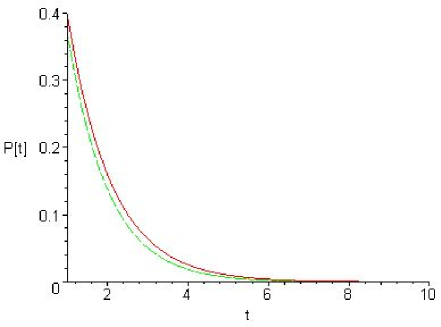
FIG. 1.: Plot on the vertical axis, commonly named $P[t]$, of the $\lambda$-corrected probability (38) (dashed line) and the harmonic probability Eq.(40) (solid line), for $\bar{\omega}=4.0\times 10^{14}/s$ and $g=\alpha\bar{\omega}$. $\alpha$ is the fine structure constant, $\alpha=1/137$ and time in units of $10^{-13}s$

IV Acknowledgements

This work has been partially supported by CNPq (Brazilian National Research Council)

REFERENCES

[1] N. P. Andion, A. P. C. Malbouisson and A. Mattos Neto,
J. Phys. A34, 3735 (2001).
[2] G. Flores-Hidalgo, A. P. C. Malbouisson and Y. W. Milla,
Phys. Rev. A65, 063414 (2002).
[3] G. Flores-Hidalgo and A. P. C. Malbouisson,
Phys. Rev. A66, 042118 (2002).
[4] B. L. Hu, J. P. Paz and Y. Zhang,
Phys. Rev. D45, 2843 (1992).
[5] C. M. Bender and T. T. Wu, Phys. Rev. Lett. 27, 461 (1971).
[6] C. M. Bender and T. T. Wu, Phys. Rev. D7, 1620 (1973).
[7] W. Thirring and F. Schwabl,
Ergeb. Exakt. Naturw. 36, 219 (1964).