Quantum Markov Channels for Qubits
Abstract
We examine stochastic maps in the context
of quantum optics. Making use of the master equation, the damping
basis, and the Bloch picture we calculate a non-unital, completely
positive, trace-preserving map with unequal damping eigenvalues.
This results in what we call the squeezed vacuum channel. A
geometrical picture of the effect of stochastic noise on the set
of pure state qubit density operators is provided. Finally, we
study the capacity of the squeezed vacuum channel to transmit quantum
information and to distribute EPR states.
pacs:
42.50.Lc, 03.67.Hk, 03.65.YzI Introduction
One of the aims of quantum information theory is to achieve the storage or transmission of information encoded in quantum states in a fast and reliable way Bennett (1998). It is unrealistic to consider a physical system, in which information is stored, as being isolated. It is well known that when the system of interest interacts with its environment, irreversible decoherence occurs, which is, in most cases, both undesirable and unavoidable Zurek (1991). This interaction causes pure states to become mixed states. This process describes the influence of noise on quantum states which results in information processing errors.
The question of how to reliably transmit information began with communication systems. Shannon’s noisy channel coding theorem is the fundamental theorem of information theory Shannon (1948); Cover (1991). It states that information can be transmitted with arbitrarily good reliability over a noisy channel provided the transmission rate is less than the channel capacity, and that a code exists which achieves this. There has been recent interest in studying quantum channels for sending quantum information and defining quantum channel capacities Holevo (1998); Lloyd (1997); Hausladen (1996); Bennett (1997); Adami (1997); Barnum (1998); Shor (2002).
As in classical information theory, a quantum channel capacity is characterized by the type of noise present in the channel. There exists a set of input states or alphabet which the sender transmits through the channel. The noise in the channel generally degrades the states. The receiver tries to recover the message which was sent from the output states. This process of induced errors may be described by a system interacting with a reservoir. For a classical communication channel, the channel is completely characterized by its transition probability matrix which determines the errors which can occur. In constrast, a quantum channel is characterized by a completely-positive, trace-preserving or stochastic map which takes the input state to an output state. This characterizes the type of noise present in the channel.
In this paper, we use a special basis of left and right damping eigenoperators for a Lindblad superoperator to calculate explicitly the image of a stochastic map for a wide class of Markov quantum channels. We use this method to derive a noisy quantum channel for qubits which we call the squeezed vacuum channel. This channel is non-unital with unequal damping eigenvalues, which makes it different from previously introduced channels Nielsen (2000). We use this channel to give geometrical insight into the Holevo channel capacity.
We begin this paper by defining a noisy quantum channel in Section II in terms of stochastic maps and the Kraus decomposition. A special case of the Markov channel is discussed. In Section III, a general Lindblad equation for a finite-dimensional Hilbert space is introduced. In Section IV, the damping basis is introduced as an alternative way to calculate explicitly the stochastic map without using a Kraus decompostion. Stochastic maps in the context of quantum optics described by a set of Bloch equations are discussed in Section V. Section VI reviews some known quantum channels and presents some more general types of channels. The stochastic map which defines the squeezed vacuum channel is explicitly calculated in Section VII and the restrictions imposed by the condition of complete positivity are presented. These results are used to determine a Kraus decomposition explicitly. The geometrical picture of the channel is given in Section VIII. Finally, Section IX deals with the channel’s ability to send classically encoded quantum states and its ability to send the resource of entanglement.
II Noisy Quantum Channels
II.1 Stochastic Maps
The concept of a noisy quantum channel arose from the field of quantum communication. Information is encoded in quantum states and transmitted across some channel where the receiver decodes the information to retreive the original message. The ability to send messages reliably depends on the noise present in the channel. The effect of the noise is to take an initial quantum state and transform it to another quantum state. The noisy quantum channel is then defined by a map
| (1) |
which takes a quantum state described by a density operator into a quantum state described by a density operator . There are certain restrictions on the class of maps which generate legitimate density operators. We require that so that unit trace of the density operator is conserved for all time. In addition, the image of the map, , must be a positive operator. A map which takes positive operators into positive operators is called a positive map. But if one considers the noise to come from a larger Hilbert space of a reservoir, then the stronger condition of complete positivity is required for the process to be physical Stinespring (1955); Choi (1972). Therefore, we restrict our attention to completely positive, trace-preserving maps which are called stochastic maps.
II.2 The Kraus decomposition
Noise in the channel may be considered as a reservoir to which the quantum state of interest is coupled. The state and the reservoir interact unitarily for some time and they become correlated. If we are now only interested in the system, we trace over the environment degrees of freedom. One may think of the reservoir as extracting information from the system as it will typically map pure states into mixed states. This noise process can be described by a quantum operation involving only operators on the system of interest. This is called a Kraus decomposition and has the form
| (2) |
where the condition
| (3) |
ensures that unit trace is preserved for all time Kraus (1983). If an operation has a Kraus decomposition, then it is completely positive. The converse is also true so that all stochastic maps have a Kraus decomposition.
II.3 The Lindblad form
The formalism we have outlined so far is general. For a important type of noise, Markov noise, we have a special class of completely positive maps. We call a Markov quantum channel one in which the noise in the channel arises from a coupling of the system with a reservoir under the Markov and Born approximations. This is a commonly used approximation in quantum optics and leads to the well-known Lindbladian form of a master equation. For this type of channel, one can always write a stochastic map as
| (4) |
The equation describes the evolution of a system coupled to a reservoir in terms of the system of interest alone. All Lindblad superoperators are stochastic maps and have a Kraus decomposition. The converse is not true in general.
In this paper, we will derive an equivalent equation for of the form
| (5) |
to obtain the image of the stochastic map for Markov noise. We use a special basis of left, , and right, , eigenoperators which allow for an explicit calculation of the stochastic map and the Kraus operators. This method works for any Markov channel.
III The General Lindblad Equation
The Schrdinger evolution of a system coupled to a reservoir can be described in terms of a master equation of the form
| (6) |
where is the density operator of the system alone, obtained by tracing over the reservoir degrees of freedom. The first term describes the coherent or unitary evolution and is simply given by the commutator
| (7) |
where H is the Hamiltonian of the undamped system.
The general form of the non-unitary part which describes the dissipation of the density operator is
| (8) |
valid for a finite N-dimensional Hilbert space. The are system operators which satisfy the conditions and . The set of complex elements form a positive matrix.
It has been proven Kossakowski (1976) that a linear operator on a finite N-dimensional Hilbert space is the generator of a completely positive dynamical semigroup in the Schrödinger picture if and only if it can be written in the form of where takes the form of Eqs. (7) and (8). We will call the generator of the semigroup which governs the dissipation the Lindbladian and denote it by . Eq. (8) may be recognized as the master equation describing irreversible evolution of an open quantum system under the Markov and Born approximations. This Lindblad equation is widely used in many branches of statistical mechanics and quantum optics. This form, the Lindblad form, has been shown to guarantee positivity and trace-preservation of the density operator Alicki (1987); Lindblad (1983).
IV The Damping Basis
There are many methods for solving master equations, the use of Fokker-Planck equations built on methods in stochastic processes, and Monte-Carlo wave functions, to name a couple Walls (1994); Gardiner (1991). In this paper, we will make use of the damping basis in order to solve a master equation which has the form of Eq. (6) containing both the coherent and damping dynamics. This amounts to solving an eigenvalue equation. In some cases, this problem can seem formidable and finding a damping basis first is useful. To solve the master equation in this fashion involves first solving the eigenvalue equation
| (9) |
for the non-unitary part of the density operator evolution describing an open system. This provides one with a complete, orthogonal basis with which to expand the density operator at any time. Such a basis is called the damping basis Briegel (1993). This basis is obtained by finding the eigenoperators of the eigenvalue equation. Likewise, the dual eigenoperators are found by solving the dual eigenvalue equation. The original basis and the dual basis are orthogonal.
If the eigenoperators of Eq. (9) are with corresponding eigenvalues then once the initial state is known
| (10) |
the state of the system at any later time can be found through
where are the damping eigenvalues and is the state dual to . These are called the left and right eigenoperators, respectively, and satisfy the following duality relation:
| (12) |
It is easy to show that L and R have the same eigenvalues. The left eigenoperators satisfy the eigenvalue equation
| (13) |
while the right eigenoperators satisfy
| (14) |
This method is a simple way of finding the density operator for a given for all times. The solution of the left and right eigenvalue equations yields a set of eigenvalues and eigensolutions: Once the damping basis is obtained, it can be used to expand the density operator. Then the density operator in this basis can be substituted back into the full Liouville Eq. (6). By doing this, one obtains a set of coupled differential equations for the coefficients of the density operator in the damping basis. Solution of this set of coupled differential equations yields the solution to the total Liouville dynamics. The important point is that once all eigenvalues and all left and right eigenoperators of the superoperator are found, the master equation can be solved and all system observables can be computed.
V Bloch Stochastic Map
When studying two-level systems there is the added advantage of a geometrical picture offered by the vector model of the density matrix. For instance, decoherence of a two-level atom is described by the dynamics of a Bloch vector with three components, , inside a unit three-sphere, governed by a set of Bloch equations Allen (1975). These constitute a set of differential equations, one for each component of the Bloch vector, of the form:
| (15) | |||||
where is the Rabi frequency, the constants and are decay rates of the atomic dipole, and is the decay rate of the atomic inversion into an equilibrium state . One typically finds that the phenomenological decay rates in the Bloch equations appear as
| (16) |
so that the parts of the atomic dipole which are in phase and out of phase with the driving field are affected in the same way by the damping. This description is in terms of a two-level atom coupled to an external field as well as a reservoir. The coupling to the external field causes the Bloch vector to rotate. The coupling to the reservoir, which might be a continuum of vacuum field modes, causes the Bloch vector to decrease in magnitude. The combination of these two behaviors leads to a spiraling in of the Bloch vector. Although we describe these dynamics in terms of the two-level atom, the Bloch picture can describe any two-level system. Here we shall consider the more general form of Eq. (V) where all three damping constants may be unequal. As we shall see, this describes the physical situation where the two-level atom is coupled to a squeezed vacuum reservoir rather than a regular vacuum field. The damping parameters lead to decoherence of the system of interest.
The decoherence is caused by the presence of noise and may be viewed as a stochastic map acting on the Bloch vector in the form of a mapping K. Wódkiewicz (2001):
| (17) |
Because there is a correspondence between the Bloch vector and the density operator , we see that the stochastic map is a superoperator which maps density operators into density operators:
| (18) |
We can expand the density operator in the Pauli basis, , and consider how the components of transform under the map. This latter transformation is characterized by a 4x4 matrix representation of . It has been found that the general form of any stochastic map on the set of complex 2x2 matrices, may be represented by such a 4x4 matrix containing 12 parameters Ruskai (2002):
| (19) |
The 3x3 block of the matrix can be diagonalized using two rotations. This amounts to a change of basis. Without loss of generality, we can consider the matrix
| (20) |
which uniquely determines the map. To preserve hermiticity, must be real. The first row must be to preserve the trace of the density operator. We call the 3x3 part of the matrix , consisting of the damping eigenvalues which are contractions, the damping matrix . Explicitly,
| (21) |
In terms of the Bloch vector, a general stochastic map may be written in the form
| (22) |
where is a translation. The overall operation consists of a damping part and translations. Due to the presence of translations, the transformation is affine.
To see the properties required by the stochastic map in terms of the Bloch vector consider the matrix representation of the Bloch vector as an expansion in terms of the Pauli matrices:
| (23) |
In the absence of noise, the Bloch vector remains on the Bloch sphere so that
| (24) |
has magnitude unity. The presence of stochastic noise transforms the matrix according to
| (25) |
To guarantee that the map transforms the density operator into another density operator, the Bloch vector can only be transformed into a vector contained in the interior of the Bloch sphere, or the Bloch ball. Equivalently, we require
| (26) |
so that the qubit density operator
| (27) |
under the map becomes
| (28) |
This is only possible if the eigenvalues are contractions. In the following sections we provide an explicit construction of the stochastic map from the Bloch Eqs. (V).
VI Two-level atom in a Squeezed Vacuum
The master equation (6) yields a plethora of possible completely positive dynamical maps. In the remainder of this paper, we wish to examine a particular form of Eq. (6) which retains a relation to the Bloch Eqs. (V) and leads to the case where the three components of the Bloch vector have different decay rates and where the Bloch vector is shifted from the origin of the Bloch sphere. As will be seen, this leads to a contraction of the set of states which lie on the Bloch sphere surface. Some states in the set become very mixed, while some remain almost pure.
We will consider a special case of the Lindbladian in Eq.(8) for a two-dimensional Hilbert space by choosing the following set of system operators :
| (29) |
where and are the qubit lowering and raising operators and is the z-component Pauli spin operator. If, along with this set of system operators, we choose the matrix elements such that
| (30) |
the resulting Lindbladian is of the form
This part of the master equation is known to describe the dissipative evolution of a two-level atom coupled to a bath Walls (1994). The raising and lowering operators describe transitions between the ground and excited states and the describe the losses caused by the reservoir and depend on phenomenological decay constants.
The coherent part of the dynamics, , will be described by the Hamiltonian
| (32) |
where is the Rabi frequency of oscillation between the ground and excited states. The full dynamics describe a two-level atom driven by a laser field subjected to irreversible decoherence by its environment. This corresponds to a linear mapping from a two-dimensional Hilbert space into a two-dimensional Hilbert space. More generally, this Liouvillian generates a completely positive dynamical map of a generic two-level system or qubit.
The Bloch equations for a two-level system described by this Lindblad operator (VI) are given by Eqs. (V) where
| (33) | |||||
The presence of the parameter is the source of the damping asymmetry between the and components of the Bloch vector. Eq. (VI) describes many well-known physical processes in quantum optics. We wish to now briefly discuss the physics behind this Lindblad form of the master equation.
VI.1 The Amplitude Damping Channel
The amplitude damping channel is identical to the case of spontaneous emission for a two-level atom. This corresponds to the following choice for the parameters:
| (34) |
The parameter A is the Einstein coefficient of spontanteous emission that depends on the density of vacuum field modes and how strongly the atom couples to the modes. This describes the exponential decay of an atom, from excited to ground state, due to vacuum fluctuations. The equilibrium state is indicating that, given enough time, the atom will be in the ground state.
VI.2 The Depolarizing Channel
Another type of noisy quantum channel is the depolarizing channel. This channel is identical to the quantum optical model for pure phase decay. This channel has parameters
| (35) |
This describes the process of phase randomization of the atomic dipole caused by atomic collisions. This leads to equal damping for the and components of the Bloch vector with contractions which depend on the parameter, , due to collisions.
VI.3 The Thermal Field Channel
In the case of spontaneous emission, the atom is coupled to a vacuum reservoir. But one can consider an atom interacting with a thermal field, so that now the field has a non-zero photon number. The reservoir may be considered as a large number of harmonic oscillators such as modes of the free electromagnetic field or a heat bath in equilibrium. In this case, one finds the decay constants are related to the photon number in the following way:
| (36) | |||||
Note that setting reduces to the case of spontaneous emission. In this thermal field case, the value of indicates that the atomic inversion approaches a steady state which is the ground state in the limit of zero photon number but as N becomes large, it approaches zero. Therefore, the equilibrium state for the inversion is bounded: One can see from Eqs. (VI) that this leads to equal damping for the and components of the Bloch vector.
VI.4 The Squeezed Vacuum Channel
A more general case occurs when all parameters are non-zero and explicitly are:
| (37) | |||||
This describes an atom in a squeezed vacuum where N is the photon number and M is the squeezing parameter. The parameter N is related to the two-time correlation function for the noise operators of the reservoir where is the field amplitude for a reservoir mode. The squeezing parameter, M, arises from the two-time correlation function involving the square of the field amplitudes . These are the familiar relations obeyed by squeezed white noise which leads to squeezing of a vacuum reservoir Gardiner (1991). A squeezed vacuum has fluctuations in one quadrature smaller than allowed by the uncertainty principle at the expense of larger fluctuations in the other quadrature. This type of reservoir leads to two dipole decay constants in the Bloch equations, the one in the squeezed quadrature being correspondingly smaller than that for the stretched quadrature.
The steady state for the inversion is the same here as in the previous case and depends only on the photon number. When the field is not squeezed (), the master equation reduces to the previous case of an atom in a thermal field. The important difference now is that the squeezing parameter has introduced a new parameter, which leads to unequal damping for the and components of the Bloch vector. In what follows, we deal with the most general case, corresponding to the Lindbladian (VI), of a qubit coupled to a squeezed vacuum reservoir. This defines a new noisy quantum channel which we call the squeezed vacuum channel (SVC) having different properties than the depolarizing and amplitude damping channels.
VII The Squeezed Vacuum Channel
VII.1 The Image of the Map
So far, we have introduced a general set of Bloch Eqs. (V) which correspond to the Liouvillian with Eq. (VI) in addition to the coherent dynamics described by in Eq. (32). We are now in a position to solve this master equation. We proceed with the method described in section IV. This tells us how the noise affects all states of the two-level system. Using the damping basis, the solution to the Liouville Eq. (9) with Lindblad operator of the form of Eq. (VI) follows. For a two-level system in a squeezed vacuum reservoir, the left eigenoperators are
| (38) | |||||
found from solving Eq. (13) while the right eigenoperators are
| (39) | |||||
found by solving Eq. (14). They correspond to the following four eigenvalues:
| (40) | |||||
Of the four eigenvalues, three of them are precisely the diagonal elements of the damping matrix (21) through the equation . We call the set the damping eigenvalues and the set , the eigenvalues (of the damping basis). This indicates a relation between the decay constants in the Bloch equations and the damping basis. The damping eigenvalues of the damping matrix contain the decay constants for the three components of the Bloch vector. The fourth of the damping eigenvalues is unity, which is a necessary condition for the density operator to have trace unity. The density operator may be expanded in any complete basis. Choosing the right eigenoperators as a basis we can write the density operator as
| (41) |
where the coefficients are obtained by projecting on to the left eigenbasis, Next we substitute the expansion on the right eigenoperators into the equation for the total Liouville operator equation and use the fact that After the substitution of into the total Liouville equation, one obtains a set of differential equations for the coefficients in the right eigenbasis and the generator of the Markovian time evolution has the following matrix representation in the same basis
| (42) |
The solution to is
| (43) |
One can perform a rotation of the right eigenbasis to obtain the following diagonalized form of the above matrix:
| (44) |
where , and the are given in Eq. (VII.1). It follows that the superoperator which maps the density operator forward in time is
| (45) |
The matrices above are represented in two different bases. Eq. (42) is in the damping basis, while Eq. (44) is in a rotated damping basis. Geometrically, one may consider the first case to be dynamics as viewed from a shifting center of the Bloch sphere. In this case, there is one affine shift towards the South pole of the Bloch sphere. This is the viewpoint in the damping basis. This can be seen by noting that in Eqs. (VII.1) for the damping basis there is one shift present in . From the right eigenoperators of the damping basis, one finds that they are almost the same as the Pauli basis. From the viewpoint of the Pauli basis, the dynamics would take place as seen from the stationary center of the Bloch sphere. In the rotated damping basis, the viewpoint is from a frame which is rotating with the driving field as well as shifting from the center of the Bloch sphere and, consequently, the eigenvalues lead to contractions or pure damping in this diagonal basis. Although the most general dynamics contains both coherent and incoherent parts, in certain situations one part may dominate the dynamics. We will consider the case where the system is not isolated from its environment but unaffected by coherent dynamics. In this case, rotations occur on a time scale much longer than the dissipation so that effectively We will see that this case is advantageous.
With these explicit formulas for the damping basis and the damping eigenvalues we can calculate the density operator for all times. This gives us the image of the map, Assuming the initial density matrix is of the form
| (46) |
we find that the stochastic map generates a new density matrix
| (47) |
in accordance with Eq. (18). This is obtained using the set the eigenoperators and eigenvalues for the damping basis. For the stochastic map which characterizes the squeezed vacuum channel, we have that the elements of are given by
| (48) | |||||
These elements are in terms of the initial density matrix elements as well as the damping eigenvalues which contain the parameters and The image gives us the density matrix after the noise operator has acted on it. The channel capacity of a noisy quantum channel is characterized by the types of errors which result after the input is transmitted. The noise operation defines the channel.
VII.2 Complete Positivity
The restriction that this map be completely positive is somewhat stringent. We have mentioned so far that the operation of on the Bloch vector must transform the vector into another vector inside the Bloch sphere. This is just one rather obvious condition. What is not as obvious is that not all states inside the Bloch sphere are allowable for the system. In other words, the Bloch vector can not access all points in the interior of the Bloch sphere. This is because of the condition of complete positivity, related to the existence of a Kraus representation which we discuss in the following section.
It has been shown Ruskai (2001) that the damping eigenvalues must obey the four inequalities
| (49) | |||
to guarantee complete positivity of the map. This is a necessary condition. These inequalities are the most general case, i.e., they apply to the damping matrix no matter which case is considered. These inequalities are a consequence of the set of equations given in the Appendix which involve the damping matrix elements . There are five such equations which, taken with the first equation, are inner products of vectors. The fact that the inner product must be positive semi-definite leads to the inequalities above. For the specific example we present, they reduce to a more familiar form. Because for spontaneous emission we have , the four inequalities become:
| (50) | |||
which are satisfied if and only if
| (51) |
In terms of the parameters M and N, this condition for complete positivity becomes
| (52) |
as expected. It is well known that M and N are not independent and the amount of squeezing is limited by the number of photons. A stricter inequality can be derived directly from the matrix elements of the Lindbladian form in Eq.(8). This must be a non-negative matrix. Using the matrix elements of Eq.(30) one finds that the c-matrix is non-negative if where N is the photon number and M is the squeezing parameter. In the case of equality, we have pure squeezing. While the general inequalities of Eq. (VII.2) are a necessary condition for complete positivity, the stricter inequality for the SVC are both necessary and sufficient.
It is worth pointing out that while contractions, without shifts, will always map the Bloch sphere into the Bloch ball, not all contractions satisfy the inequalities (VII.2). Those which do not satisfy them, do not have a Kraus representation and, hence, are not completely positive maps. We shall see that the condition of complete positivity restricts the allowable ellipsoids of the image. Because the Lindblad form of the master equation guarantees complete positivity, by Kraus’ theorem there must exist a decomposition with Kraus operators which acts on the system of interest alone. In the next section, we give an explicit form of the Kraus operators.
VII.3 The Kraus Decomposition
For the special case of a qubit there can be at most four Kraus operators. To see why this is true, the reader is referred to a lemma where it is shown that the minimum number of Kraus operators is equal to the rank of a certain matrix Ruskai (2001). It follows that the minimum number of Kraus operators needed to represent the map for the squeezed vacuum channel is four. We do not show this, but rather, use this fact to find an operator-sum representation using the minimum number of Kraus operators possible. We start by assuming that the four Kraus operators exist and that they are real, although in general they are represented by complex matrices. Next we expand all 2x2 matrices in Eq. (2) in the Pauli basis. If we let
| (53) | |||||
then Eq. (2) becomes Equating each coefficient in and leads to a set of linear equations which underdetermine the sixteen coefficients of the Kraus operators in Eq. (53) in the Pauli basis. Thus, the Kraus representation is not unique. The elements of the Kraus operators can be written as vector components
| (54) |
where j=0,1,2,3. The set of linear equations which need to be satisfied is given in the Appendix. The stochastic map for the squeezed vacuum channel(47) has Kraus operators which can be realized in the following way:
| (55) | |||||
with constants given by
| (56) | |||||
The Kraus decomposition is not unique so a different set of four Kraus matrices can represent the same map. The minimum number of Kraus operators, for the map constructed here, is four, but one could just as well use more than four to produce the map. This freedom in the Kraus decomposition is related to the many possible ways of performing measurements on the system. The system is decohered as a result of being measured by the environment. The many different Kraus operators correspond to the many different positive operator-valued measures (POVMs) which lead to the decohered state. This is why there are many different sets of possible Kraus operators which would result in the same map .
One can verify that this choice of Kraus operators satisfies the condition in Eq. (3) so that the final density operator has trace unity. This is a necessary condition for a trace-preserving map, to which we restrict ourselves. However, one could consider maps which are not trace-preserving in which case Eq. (3) becomes an inequality. Since the map is non-unital, i.e., it does not map identity into identity, we have
| (57) |
This is due to the presence of the affine shift. Next, we discuss what all this means geometrically in terms of the Bloch sphere.
VIII The Geometrical Picture
For a set of general Bloch equations and a Lindbladian there exists a 4x4 matrix of the form (20). For the Lindblad equation we have considered here, this map can also be expressed, in terms of the 4x4 matrix, as
| (58) |
This is a special case of Eq. (20) with
| (59) |
and affine shifts
| (60) |
From this we see that the components of the Bloch vector are contracted. To guarantee that the Bloch vector is contained within the Bloch ball the following condition must hold:
| (61) |
Furthermore, we see that the matrix (58) transforms the Bloch sphere into an ellipsoid inside the Bloch ball. That is, the image of the set of pure state density matrices under the stochastic map is given by the family of ellipsoids
| (62) |
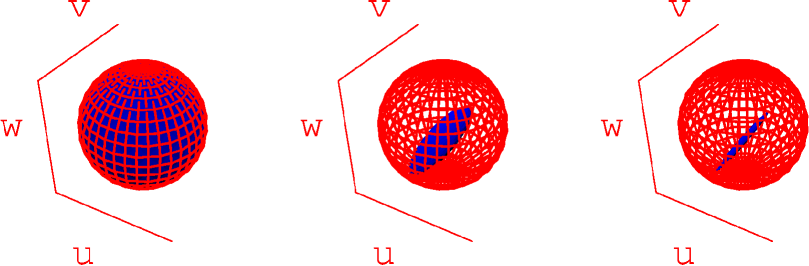
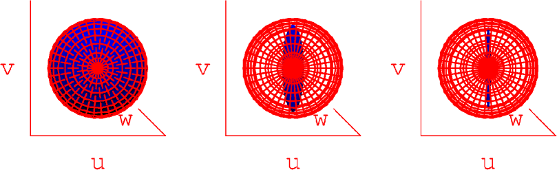
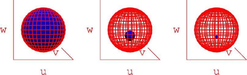
The shift, determines the center of the ellipsoid while the eigenvalues, define the lengths of the axes. If we start with the set of pure state density operators which lie on the Bloch sphere, then as time progresses, the states move onto the surface of a contracting ellipsoid. The pure states have become mixed states. By Eq. (59), each axis is unequally contracted, as shown in Figure 1. Because of the squeezed vacuum, the -component experiences very little damping while the -component is rapidly damped, as shown in Figure 2. The explicit expression for the shift in terms of indicates the ellipsoid is translated in the negative -direction over time and settles into an equilibrium or fixed point, as shown in Figure 3.
The matrix of Eq. (20) is in the Pauli basis and describes the dissipative dynamics from the stationary viewpoint at the center of the Bloch sphere. From this viewpoint, one would observe a contracting ellipsoid moving away from the Bloch sphere center to some equilibrium point. The matrix could also be represented in the damping basis, in which case it would be diagonal. This amounts to transforming to a frame where, instead of being a stationary observer at the Bloch sphere center, one is moving along with the shifting ellipsoid. In this case, one observes only a contracting ellipsoid. This is the geometrical picture of the damping basis.
If the effect of noise on all input states is known, then the least noisy output states can be identified. The minimal entropy states are the states least affected by the noise and consequently the least-mixed states. Geometrically, these would be all states whose distance to the surface of the Bloch vector is a minimum. These states form a set of extreme points of the convex set of density operators. Such a set of points on the ellipsoid having minimal distance to the Bloch sphere may consist of one or two points, a circle, or the entire surface of the ellipsoid. For a given noise, these nearest points represent states of maximum purity in the set of states affected by the noise. For the squeezed vacuum channel, the set of minimal entropy states consists of two states along the major axis of the ellipsoid.
The purest minimal entropy states are obtained by maximal squeezing of the reservoir. This results in the most eccentric ellipsoid which is stretched in one particular direction and places the two points along the major axis of the ellipsoid close to the Bloch sphere surface, as seen in Figure 1. As the squeezing parameter goes to zero, the ellipsoid becomes less elongated and the minimal entropy states lose their purity. When M is identically zero, the minimal entropy points lie in a circle. Equivalently, as M approaches zero, the damping for the component of the Bloch vector approaches that for the component.
If we had included the coherent dynamics as well as the dissipative dynamics, the minimal entropy points on the ellipsoid would be more mixed than without the coherent dynamics. The reason for this is that the ellipsoid would begin to rotate and the minimal entropy points along the -component would rotate away from this axis where there is more noise. Consequently, the minimal entropy points get degraded by being moved away from the axis with least noise so that for this channel, it is advantageous to keep coherent dynamics suppressed.
Other noisy quantum channels have been introduced such as the depolarizing channel, amplitude-damping channel, and the phase-damping channel Nielsen (2000). The depolarizing channel has all three components of the Bloch sphere equally damped and it is a unital channel. The set of minimal entropy points would lie on a sphere. The amplitude-damping channel has two of the three components equally damped and it is a non-unital channel. It arises from the master equation describing spontaneous emission as in Eq. (34). The set of all states moves on an ellipsoid which shifts toward the South pole. The phase-damping channel is the case described in Eq. (35). It has two equally damped components, one undamped component, and it is unital. It has two extreme points, one at the North pole and one at the South pole. Given any type of noise, the geometrical picture is a useful aid and allows for a simple analysis of the channel capacity. To transmit information over the channel it is ideal to use as input states those states which result in the minimum amount of measurement error.
IX Channel Capacity
IX.1 Encoding Classical Information in Qubits
One way to use a quantum channel is to send classical information encoded in quantum states. Although quantum information is being sent because qubits are sent through the channel, these qubits are being used in an entirely classical way. A natural extension of classical channel capacity for a quantum channel has been proposed by Holevo Holevo (1998). In this case, quantum states are used to transmit messages reliably across some noisy quantum channel. Also known as the product state capacity, because messages are sent using tensor products of the input states which comprise the alphabet, the channel capacity for classical information over a noisy quantum channel has been defined as
| (63) |
S is the von Neumann entropy defined as and is the quantum analogue of the Shannon entropy. The maximum is taken over all possible ensembles of input states. The input alphabet consists of a set of states which are transmitted with probability . For the case of the SVC, the maximization is achieved using the two orthogonal input states for which the damping is smallest with a uniform distribution over these states. With the convention already chosen, this is the v-component of the Bloch sphere. Thus, the optimal way to send classical information through the SVC is to prepare product states using the two orthogonal input states and ,which lie in the equatorial plane of the Bloch sphere, with corresponding probabilities and to encode messages. For example, , requiring N uses of the channel, would represent the N-length classical bit string 011.
The noise operation causes the output of these two states to be non-orthogonal, mixed states. No single measurement at the receiving end can perfectly determine which input state was sent. There are two errors which can occur, one error arises because of the non-distinguishability of non-orthogonal states while the other arises because the state is mixed. The first term in Eq. (63) takes into account the information loss due to the fact the the output states are non-orthogonal while the second term takes into account the fact the the output states are mixed. The Holevo capacity has a nice geometrical interpretation. To see this we consider an example. For simplicity, let us assume that the SVC has maximum squeezing and the input states are received after a one second pass through the channel. Then, using the same parameters as in Figures 2-4, namely, N=1,M=, and t=1, we find explicitly that the Holevo capacity is C(SVC)=.93-.11=.82 qubits per transmission. This is calculated by using and as input states with corresponding probabilities and and calculating the quantity inside the brackets of Eq. (63).
Note that the first term is present because of the affine shift while the second term is due to a contraction of the Bloch sphere. To see the various errors which can occur we can write C(SVC)=1-(1-.93)-.11=.82 qubits per transmission. Now the first term is the number of qubits which can be sent if there was no noise present. The second term is the error caused by the affine shift. This is a distance from the center of the Bloch sphere to the center of the ellipsoid. This error occurs because the states lose their orthogonality. The last term is the error due to the contraction of the ellipsoid. The contractions cause the states to become mixed and consequently there will be measurement errors of this kind. This term is a distance from the Bloch sphere surface to the surface of the ellipsoid. It is interesting to note that the affine shift actually takes the maximally mixed state into a state with less entropy. This can occur because generalized measurements can decrease entropy. Also, if no noise were present the capacity would be C(I)=1 qubit per transmission meaning that one error-free qubit can be transmitted in one use of the channel.
IX.2 Entanglement Transmission
Another way in which a quantum channel can be used which does not have a classical counterpart is for entanglement transmission. In this case, one is interested in distributing parts of an entangled state to different locations. For example, a source may generate EPR pairs and one may be interested in sending one half of this EPR pair through some channel to a receiver. Naturally, noise will corrupt the transmitted state and lead to a decrease in the entanglement of the joint state.
A channel has the capacity to transmit entanglement if after passing through the channel there is any nonzero entanglement present in the joint state. It has been shown by Horodecki et. al that any nonseparable bipartite system which has entanglement, however small, can be distilled to a singlet form Horodecki (1997). Therefore, if a channel can transmit any entanglement, it is a useful channel. N copies can be sent and a singlet state can be distilled.
Assuming the initial Bell state has the following density operator representation
| (64) |
The output state will be determined by the following operation
| (65) |
which describes the process of sending one qubit to Bob while Alice keeps her qubit intact. In matrix notation, the output state for the joint system is
| (66) |
At the initial time the joint state is maximally entangled and the noise process should result in a decrease in the entanglement until some critical time when the joint state is separable and remains separable thereafter. Using the Peres criterion of the positivity of the partial transpose, one can determine when the state becomes separable Peres (1996). A necessary and sufficient condition for the output state to be nonseparable is that the partial transpose map be negative Horodecki (1996). To check the positivity of the partial transpose it suffices to examine the eigenvalues of the operator given by
| (67) |
where denotes the transpose of the state of Bob’s qubit. The four eigenvalues of the partial transpose matrix are
| (68) | |||||
Initially, the eigenvalues have values and while in steady state they become and . We find that the nonseparability is determined solely by the eigenvalue . The transmitted EPR state remains nonseparable provided
| (69) |
There is some critical time when the eigenvalue is zero and then remains positive thereafter. The value of this critical time depends on the parameters of the reservoir. As the photon number of the reservoir increases the critical time decreases. One would expect this to be the case since the reservoir is more noisy. It is not as obvious what the effect of the squeezing of the reservoir has on the entanglement because the squeezing results in a tradeoff of more noise in one component and a decrease in another component. We find that a squeezed reservoir results in a longer entanglement time for the inital maximally entangled state. The critical time is longer for a maximally squeezed vacuum. This is shown by the solid curve in Fig. 4.

In both the case of sending product states and for distributing EPR states, the squeezing parameter, M, is able to enhance the capacity of the channel.
X Conclusion
In this paper we provided a method for calculating a stochastic map for any quantum Markov channel. Our method uses a special damping basis of left and right eigenoperators. This basis provides a natural way to generate noisy quantum channels from a quantum optical approach. This technique allows one to calculate the stochastic map and from this one can then determine a set of Kraus operators which define the noisy quantum channel.
We used this method to calculate explicitly a noisy quantum channel we called the squeezed vacuum channel. We showed the relationship between a set of quantum optical Bloch equations and the damping basis. Some known quantum channels such as the amplitude-damping channel and the depolarizing channel arise from this set of Bloch equations. These quantum Markov channels are special cases of the squeezed vacuum channel. The channel we derived is a non-unital stochastic map which is characterized by three unequal damping eigenvalues. By using the damping basis, we were able to find a set of Kraus operators for the stochastic map. From this, the effect of noise on the set of input states was interpreted geometrically. The Bloch picture was used to study the effect of noise present in the channel and the coherent dynamics was considered in addition to the incoherent dynamics.
The procedure to calculate the channel capacity requires a maximization over all input states. Using the Bloch picture, we were able to determine the channel capacity for the squeezed vacuum channel to transmit classical information in quantum states. We found that the channel has two minimal entropy points which should be used to optimally transmit information. A geometrical interpretation of the Holevo capacity was given and used to identify two types of errors–those arising from non-orthogonal states and those arising from mixed states. We also discussed the ability of this channel to distribute EPR states. We found that, after sending one half of the EPR state through the channel, there is some critical time after which the state becomes separable.
This paper shows that with the a priori knowledge of the effect of noise given by a Lindblad form, one can choose to encode messages using the pure states which are closest to the final states of minimum entropy. The squeezed vacuum channel is a more general noisy channel derived from quantum optical two-level systems. Unlike previously introduced channels, it has unequal damping eigenvalues and it is non-unital. We found that channel capacity is enhanced by the squeezing parameter, M, whether it is used to send product states or used to transmit EPR states. This channel may prove useful as a testing ground for future conjectures on quantum channel capacities.
Acknowledgements.
We thank Dr. G.H. Herling for discussions and corrections to the final draft. This work was partially supported by a KBN grant No. 2PO3B 02123 and the European Commission through the Research Training Network QUEST.XI Appendix
For the Hilbert space of 2x2 matrices, one may always represent the quantum channel using four or less Kraus operators. To find a representation, one can construct a set of simultaneous equations via the prescription given in Section VI.B. The squeezed vacuum channel has Kraus operators which must satisfy the following set of equations. There are four for the shifts:
| (70) | |||||
For the coefficients of and
| (71) | |||||
And to satisfy the condition :
| (72) |
The set of equations leads to restrictions on the damping eigenvalues as in Eq.(VII.2). As an example of the explicit construction of Kraus matrices, we will consider the pure phase decay case of Eq.(35) which is the phase-damping channel. For this case, and and . Any solution of the set of linear equations along with these conditions will give a Kraus representation. The following solution for elements of the Kraus matrices is easily found to be , and
| (73) |
with
| (74) |
The phase-damping channel has a Kraus representation given by:
| (75) | |||||
| (76) |
References
- Bennett (1998) C.H. Bennett and P.W. Shor, IEEE Trans. Inf. Theory, 44, No. 6, 2724, (1998).
- Zurek (1991) W.H. Zurek, Phys. Today, 44, 36 (1991).
- Shannon (1948) C.E. Shannon, Bell Sys. Tech. Journal, 27, 379,623-656 (1948).
- Cover (1991) T. Cover and J. Thomas, Elements of Information Theory, (Wiley, (1991)).
- Hausladen (1996) P. Hausladen, R. Jozsa, B. Schumacher, M. Westmoreland, and W. Wooters, Phys. Rev. A, 54, No. 3, 1869, (1996).
- Bennett (1997) C.H. Bennett, D.P. DiVincenzo, and J.A. Smolin, Phys. Rev. Lett., 78, No. 16, 3217, (1997).
- Adami (1997) C. Adami and N.J. Cerf, Phys. Rev. A, 56, No. 5, 3470, (1997).
- Barnum (1998) H. Barnum, M.A. Nielsen, and B. Schumacher, Phys. Rev. A, 57, No. 6, 4153, (1998).
- Shor (2002) P. Shor, LANL e-print quant-ph/0201149.
- Holevo (1998) A.S. Holevo, Russian Math Surveys, 53, 1295 (1998).
- Lloyd (1997) S. Lloyd, Phys. Rev. A, 55, 1613 (1997).
- Nielsen (2000) M.A. Nielsen and I.L. Chuang, Quantum Computation and Quantum Information, (Cambridge University Press, (2000)).
- Stinespring (1955) W.F. Stinespring, Proc. Amer. Math. Soc., 6, No. 2, 211 (Apr., 1955).
- Choi (1972) M. Choi, Can. J. Math., 24, No. 3, 520 (Jan., 1972).
- Kraus (1983) K. Kraus, States, Effects and Operations: Fundamental Notions of Quantum Theory, (Springer-Verlag (1983)).
- Kossakowski (1976) V. Gorini, A. Kossakowski, and E.C.G. Sudarshan, J. Math. Phys., 17, No. 5, 821, (1976).
- Alicki (1987) R. Alicki and K. Lendi, Quantum Dynamical Semigroups and Applications, (Springer-Verlag (1987)).
- Lindblad (1983) G. Lindblad, Non-Equilibrium Entropy and Irreversibility, (D. Reidel Publishing Company (1983)).
- Walls (1994) D.F. Walls and G.J. Milburn, Quantum Optics, (Springer-Verlag, (1994)).
- Gardiner (1991) C.W. Gardiner, Quantum Noise, (Springer-Verlag (1991)).
- Briegel (1993) H.J. Briegel, B.-G. Englert, Phys. Rev. A47, 3311 (1993).
- Allen (1975) L. Allen and J.H. Eberly, Optical Resonance and Two-Level Atoms, (Wiley, (1975)).
- K. Wódkiewicz (2001) K. Wódkiewicz, Opt. Express 8, No. 2, 145 (2001).
- Ruskai (2002) M.B. Ruskai, E. Werner, and S. Szarek, Linear Algebra Appl., 347, 159 (May, 2002).
- Ruskai (2001) C. King and M.B. Ruskai, IEEE Trans. Inf. Theory, 47, No. 1, 192 (Jan., 2001).
- Horodecki (1997) M. Horodecki, P. Horodecki and R. Horodecki, Phys. Rev. Lett., 78, No. 4, 574 (1997).
- Peres (1996) A. Peres, Phys. Rev. Lett.,77, No. 8, 1413 (1996).
- Horodecki (1996) M. Horodecki, P. Horodecki and R. Horodecki, Phys. Lett. A, 223, 1 (1996).